Cross-Layer Design for Lifetime Maximization in ... - CiteSeerX

SUBMITTED TO THE IEEE TRANS. ON WIRELESS COMMUNICATIONS

1

Cross-Layer Design for Lifetime Maximization in Interference-Limited Wireless Sensor Networks Ritesh Madan, Shuguang Cui, Sanjay Lall, and Andrea Goldsmith

Abstract We consider the joint optimal design of the physical, medium access control (MAC), and routing layers to maximize the lifetime of energy-constrained wireless sensor networks. The problem of computing lifetime-optimal routing flow, link schedule, and link transmission powers for all active time slots is formulated as a non-linear optimization problem. We first restrict the link schedules to the class of interference-free time division multiple access (TDMA) schedules. In this special case, we formulate the optimization problem as a mixed integer-convex program, which can be solved using standard techniques. Moreover, when the slots lengths are variable, the optimization problem is convex and can be solved efficiently and exactly using interior point methods. For general non-orthogonal link schedules, we propose an iterative algorithm that alternates between adaptive link scheduling and computation of optimal link rates and transmission powers for a fixed link schedule. The performance of this algorithm is compared to other design approaches for several network topologies. The results illustrate the advantages of load balancing, multihop routing, frequency reuse, and interference mitigation in increasing the lifetime of energyconstrained networks. We also briefly discuss computational approaches to extend this algorithm to large networks.

An intial version of this paper was presented at IEEE INFOCOM in March 2005. R. Madan and A. J. Goldsmith are with the Department of Electrical Engineering, Stanford University, Stanford, CA 94305. Emails: [email protected], [email protected]. S. Cui is with the Department of Electrical and Computer Engineering, University of Arizona. Email: [email protected]. S. Lall is with the Department of Aeronautics and Astronautics, Stanford University, Stanford, CA 94305. Email: [email protected].

SUBMITTED TO THE IEEE TRANS. ON WIRELESS COMMUNICATIONS

2

I. I NTRODUCTION We consider a network of wireless sensor nodes distributed in a region. Each node has a limited energy supply and generates information that needs to be communicated to a sink node. We assume that each node can vary its transmission power, modulation scheme, and duty cycle. The focus of this paper is on the computation of optimal transmission powers, rates, and link schedule that maximize the network lifetime. We consider a scenario where the data rates supported by the network are high; an example of such a network is a video surveillance network. Transmission at high data rates necessitates the use of high transmission powers on the wireless links. This leads to many links interfering strongly with each other. Hence, link scheduling to mitigate interference becomes an important and challenging task. The network is considered to be alive as long as all nodes have some energy; the lifetime is taken to be the earliest time at which a node runs out of energy. We will use the term transmission scheme/strategy to refer to the data rates, transmission powers, and link schedule for a network. For energy-constrained wireless networks, we can increase the network lifetime by using transmission schemes that have the following characteristics. (1) Multihop routing: In wireless environments the received power typically falls off as the mth power of distance, with 2 ≤ m ≤ 6. Hence, we can conserve transmission energy by using multihop routing [1], [2]. (2) Load Balancing: If a node is on the routes of many source destination pairs, it will run out of energy very quickly. Hence, load balancing is necessary to avoid the creation of hot spots where some nodes die out quickly and cause the network to fail [3]. (3) Interference mitigation: Links that strongly interfere with each other should be scheduled at different times to decrease the energy consumption on these links [4]. (4) Frequency reuse: Weakly interfering links should be scheduled simultaneously so that each link can transmit at a lower rate when active. This reduces the average transmission power on each link [5]. We note that there is an inherent trade-off between using minimum energy routes and load balancing. Minimum energy routing may require some nodes to lie on routes of many source destination pairs, which may cause them to run out of energy quickly. The network lifetime can be increased by load balancing, where a part of the data may be transmitted over energy suboptimal paths. In addition, there is a trade-off between scheduling each link

SUBMITTED TO THE IEEE TRANS. ON WIRELESS COMMUNICATIONS

3

for a larger amount of time to decrease energy consumption for data transmission and interference mitigation by scheduling strongly interfering links at different times. A. Prior Work Cross-layer design for throughput maximization has received much attention over the past few years. Achievable rate combinations for wireless networks were computed in [6]. Throughput maximization through joint design of power control, link scheduling, and routing layers was considered in, for example, [7], [8], [9], [10], [11]. The design challenges and the importance of cross-layer design for meeting application requirements in energyconstrained networks were described in [12]. For wireless sensor networks, we may not always need to operate on the boundary of the achievable rates region. Hence, we have a choice among various transmission strategies (routing, power control, and scheduling) that we can exploit to increase the lifetimes of such networks. An overview of the synergy between the various layers was given in [13]. A brief overview of recent work on optimization of different layers of a wireless network for minimizing energy consumption and maximizing network lifetime is given below. (1) Physical Layer: For a given rate vector, power control can be used to conserve energy. An overview of power control was given in [14]. Energy-optimal modulation schemes for coded and uncoded systems were studied in [5], where given the number of bits to transmit with a certain deadline, an optimal constellation size was computed to minimize the total transmission and circuit energy. Also, it was shown that if we relax the constraint that the constellation size is an integer, the energy minimization problem can be approximated by a convex optimization problem. (2) MAC: The physical layer results in [5] were extended in [15] to compute the TDMA time slot lengths to minimize the total energy consumption in a network consisting of many transmitters and one receiver. However, the problem of deciding the allocation of time slots becomes combinatorial when we consider an arbitrary wireless network, and allow interfering links to be scheduled in the same time slot. (3) Routing: Routing algorithms for wireless networks have traditionally focused on minimizing the total energy consumption. However, as pointed out in [3], this can lead to some nodes in the network being drained of energy very quickly. Hence instead of trying to minimize the total energy consumption, routing to maximize

SUBMITTED TO THE IEEE TRANS. ON WIRELESS COMMUNICATIONS

4

the network lifetime was considered in [3]. Distributed algorithms to compute a routing scheme to maximize the network lifetime were proposed in [3], [16], [17], [18]. (4)

Cross-layer: Joint scheduling and power control to reduce energy consumption and increase single hop throughput was considered in [19]. Cross-layer design based on computation of optimal power control, link schedule, and routing flow was described in [4]. The maximum achievable rate was assumed to be a linear function of signal to noise and interference ratio (SINR) and the goal was to minimize the total power consumption over an infinite horizon. The routing flow was computed in an incremental manner: it used the Lagrange multipliers obtained at each step by solving an optimization problem of possibly exponential complexity in the number of links. Energy efficient power control and scheduling, with no rate adaptation on links, for QoS provisioning were considered in [13]. Cross-layer design with emphasis on detailed modeling of circuit and transmission energy, and restriction of MAC to variable length TDMA was described in [20]. Joint routing, power control, and scheduling for a TDMA-CDMA network was considered in [21].

We consider a slotted time model, and guarantee the satisfaction of average rate requirements over a predefined frame duration; this is similar to the model in [13]. We note that a slotted model enables us to use a link schedule that mitigates interference by scheduling strongly interfering links in different slots. Thus it is more general than the model in [22]. Also, the algorithm in [22] assumes that a feasible solution can be computed where each link has a signal to interference and noise ratio (SINR) of at least 1. This is highly unlikely in a network with many nodes and high data rates where many links will strongly interfere with each other. Moreover, the algorithm in [22] is for a single slot and does not extend to a slotted time model. We build on some of the ideas in [7], [22] to design our adaptive link scheduling algorithm; however, we note that the generalization is non-trivial and requires new methods and insights. As in [4], [13], we use a realistic model of the interference between all links that transmit simultaneously. This is more general than the interference model considered in [21], where the schedule for links in the same neighborhood was assumed to be orthogonal, and interference from distant links was neglected. For the special case of orthogonal link schedules, we compute the exact optimal transmission strategy. Also, unlike in [13], we consider rate adaptation on links and a fixed bit error rate (BER) requirement. As shown in [5], rate adaptation

SUBMITTED TO THE IEEE TRANS. ON WIRELESS COMMUNICATIONS

5

can lead to significant decrease in energy consumption. However, allowing for rate adaptation on links makes the problem considerably more complex. We no longer have a linear constraint on transmission powers [13] that guarantees an SINR greater than a threshold. Instead we have a non-linear and non-convex constraint on the rate and power of each link (see Section 2.4 for details). In addition, we consider joint routing along with link scheduling and power control (with rate adaptation). Also, instead of minimizing the total average power consumption over the network, we maximize the network lifetime.

B. Contributions Our main contribution is a computational algorithm for cross-layer optimization in a very general setup. The algorithm computes competitive solutions that increase network lifetime for wireless networks with high bandwidth efficiency. This is in contrast to [4], where the authors assume a system with very low bandwidth efficiency.1 . The solutions computed by our algorithm are much better than commonly used heuristics. The algorithm alternates between link scheduling and computation of transmission powers and rates. The transmission scheme computed during each iteration is feasible. Hence, the suboptimality of the solution can be traded off with the required computational power. The main step of our algorithm involves the solution of a convex optimization problem for which the number of variables grows as 2LN , where N is the number of slots and L is the number of links in the network. Also, the number of constraints grows as N L + 2|V |, where |V | is the number of nodes in the network.

C. Outline The next section lists our assumptions about the wireless network and formally defines the problem of computing the transmission powers, data rates, and link schedule to maximize the network lifetime, as an optimization problem. We show how to solve this problem exactly if we restrict the MAC layer to only TDMA schemes (interference-free case). In Section III, we consider the general case and find a convex approximation to the problem of computing an optimal data rate and transmission power, for each link and time slot, and a fixed link schedule. Then we describe an algorithm that uses a heuristic to adapt the link schedule to the resulting optimal rates and powers. 1

By bandwidth efficiency, we refer to the ratio of the data rate to the total bandwidth in the system. For CDMA systems, the bandwidth

under consideration is that after spreading.

SUBMITTED TO THE IEEE TRANS. ON WIRELESS COMMUNICATIONS

6

Section IV describes the results of numerical studies of the algorithm for different network topologies. The results also illustrate the advantages of frequency reuse, interference mitigation, load balancing, and multihop routing in energy-constrained wireless networks. Section V gives conclusions and possible directions for future work. II. P ROBLEM D EFINITION A. System Model We consider a static wireless network. We assume that a link exists from node i to node j , if the received power at node j when node i transmits at maximum power, is greater than a predefined threshold. Note that, in general, we can consider a very low threshold; this would correspond to a fully connected network. However, this introduces many links in the network graph and hence, many optimization variables, making the cross-layer optimization problem very complex. By introducing a reasonable threshold, we do not consider links that are very weak – these links will not only consume a lot of power, but also cause a lot of interference to other links. For an information theoretic justification we refer the reader to [23]. The channel over each link is an additive white Gaussian noise (AWGN) channel with fixed noise power. Also, we assume a deterministic path loss model where the power falls off as dm for distance d, with 2 ≤ m ≤ 6. The maximum rate per unit bandwidth that can be supported over a link with SINR γ is r = log(1 + Kγ), where K = −1.5/(log(5BER)). This is a good model for modulation schemes such as MQAM with constellation size greater than or equal to 4 [24]. For notational convenience we will consider r to be in nats/Hz/s, i.e., we use the natural logarithm. We assume that a link can vary the constellation size over

each time slot. We relax the constraint that the constellation size is an integer, i.e., we allow r to take all values in R+ . At any given time, a node can either transmit to, or receive from, at most one other node in the network. For the MAC layer, we assume that the network time shares between different transmission modes in a periodic fashion. The schedule is periodic with N time slots; during each slot the network uses one transmission mode – i.e. one set of powers and rates over each link. Also, the flow conservation equations are satisfied over every frame of N time slots. In this paper, we restrict ourselves to the case of single commodity flow. We note that the methods

in this paper can be easily extended to the case of multicommodity flow; the number of variables grow linearly with the number of commodities. If a node transmits at power P , the power consumption in the power amplifier circuit is given by (1 + α)P . The parameter α > 0 represents the inefficiency of the power amplifier; we take α

SUBMITTED TO THE IEEE TRANS. ON WIRELESS COMMUNICATIONS

7

to be a constant [25]. The power consumption values of the transmitter circuit (other than the amplifier) and the receiver circuit are modeled as constants Pct and Pcr , respectively [5].

B. Notation We define the following notation. 1) G = (V, L) denotes the directed graph representing the network. V is the set of wireless nodes and L is the set of directed links. Let A ∈ R|V |×|L| be the     1     A(v, l) = −1        0

incidence matrix of the graph G . We have if v is the transmitter of link l if v is the receiver of link l otherwise

Let us write A = A+ − A− , such that A+ (v, l), A− (v, l) = 0 if A(v, l) = 0, and A+ , A− have only 0 and 1 entries. 2) Let N be the number of time slots in each frame of the periodic schedule. Ln denotes the set of links scheduled, i.e., allowed to transmit, during time slot n ∈ {1, . . . , N }. 3) Pln and rln denote the transmission power and rate per unit bandwidth, respectively, over link l and slot n. Also, rn , P n ∈ R|L| will be used to denote the corresponding vectors for time slot n. Let Plmax be the maximum

allowable transmission power of the transmitting node of link l. The corresponding vector is P max ∈ R|L| . Also, define the vectors 1t (P n ), 1r (P n ) ∈ R|V | such that       + T n T n  1 if (av ) P > 0  1 if (a− v) P >0 n n (1t (P ))v = (1r (P ))v =      0 otherwise  0 otherwise T − T + − where (a+ v ) and (av ) denote the v th row of the matrices A and A , respectively. Thus the vectors give

the sets of nodes that transmit and receive data, respectively, in each time slot. 4) Let E ∈ R|V | be such that Ev denotes the initial amount of energy at node v . Pct and Pcr give the power consumption of the transmitter and the receiver circuits at a node, respectively. These values are assumed to be the same across all nodes. 5) Let sv denote the rate at which information is generated at node v . Let s ∈ R|V | be the vector whose entries are sv . We note that ssink = −

P

v∈V,v6=sink sv .

SUBMITTED TO THE IEEE TRANS. ON WIRELESS COMMUNICATIONS

8

6) G ∈ R|L|×|L| is the link gain matrix of the network. Glk denotes the power gain from the transmitter of link k to the receiver of link l. Note that in order to prevent a node from transmitting and receiving simultaneously, we can set very high values for the gain entries of G corresponding to each pair of links originating and terminating at a node. The computational algorithm will then prevent these links from being scheduled simultaneously. Let N0 denote the total noise power over the bandwidth of operation.

C. Network Lifetime Let Tv denote the lifetime of node v , i.e., the time at which it runs out of energy. Then the network lifetime is defined to be Tnet = minv∈V,v6=sink Tv . Note that this is a standard definition of network lifetime used in, for example, [3], [16], [17]. This definition makes the analysis tractable for many different scenarios. Another interpretation of the optimization problem that maximizes the time at which the first node dies is that it minimizes the maximum ratio of average power consumption to initial energy among all nodes – it thus balances the data flow in the network such that no node incurs a very high power consumption. Hence, for a large network with many redundant nodes, a suboptimal but reasonable approach would be to use the transmission scheme that maximizes the time at which the first node dies, and recompute the transmission scheme once the topology has changed significantly after many nodes run out of energy. Until then, the same transmission scheme can be used with greedy readjustment of flows. For a more detailed discussion on network lifetime definitions and associated distributed algorithms for routing, we refer the reader to Section VII of [18]. We note that for each optimization problem (to maximize the network lifetime) formulated in this paper, we can formulate a similar corresponding optimization problem to minimize total energy. Hence, the techniques in this paper can be used for energy minimization in the network as well.

D. Optimization Problem We now formulate an optimization problem to maximize the network lifetime. We have the following constraints. (1) Flow Conservation: The flow conservation equations are satisfied over each frame of N time slots. (2) Rate Constraints: The maximum rate that can be sent over each link is (1+K log SINR). (3) Energy Conservation: The energy consumed by each node over time Tnet should be less than or equal to the initial energy at the node. (4) Range

SUBMITTED TO THE IEEE TRANS. ON WIRELESS COMMUNICATIONS

9

Constraints: The flow over a directed link can only be from the transmitter to the receiver. The transmission power at a node is less than or equal to the maximum transmission power at that node. Then, the problem of maximizing the network lifetime can be written as the following optimization problem. Tnet

max.

1 A(r1 + . . . + rN ) = s N Ã ! Gll Pln log 1 + K P ≥ rln n k6=l Glk Pk + N0

s.t.

N ´ Tnet X³ (1 + α)A+ P n + Pct 1t (P n ) + Pcr 1r (P n ) ¹ E N n=1

rn º 0,

0 ¹ P n ¹ P max

for all n = 1, . . . , N and l ∈ L. The variables are Tnet , rln , Pln , for n ∈ {1, . . . , N }, l ∈ L. Thus the solution gives optimal transmission modes during the N time slots of each frame, i.e., optimal transmission powers and rates over each link during each time slot. As in [18], we can use a change of variable q = 1/Tnet , to write the problem as the following equivalent optimization problem. q

min. s.t.

A(r1 + . . . + rN ) = N s ! Ã Gll Pln ≥ rln log 1 + P n+N G P 0 lk k6=l k rn º 0,

(1)

0 ¹ P n ¹ P max

N ³ ´ X (1 + α)A+ P n + Pct 1t (P n ) + Pcr 1r (P n ) ¹ qN E n=1

We have absorbed the system constant K into the diagonal entries of G. Both the optimization problems considered in this section are not convex optimization problems. In particular, for the above problem, the rate constraint on each link for each slot cannot be rearranged to be written as some convex function f (r, P, q) ≤ 0. We will first reduce the problem to a mixed integer-convex problem for TDMA link schedules. For the more general case of arbitrary link schedules, we will use an iterative approach that alternates between computation of rates and powers, and adaptation of the link schedule.

SUBMITTED TO THE IEEE TRANS. ON WIRELESS COMMUNICATIONS

10

E. Optimal TDMA Schemes The problem in (1) when restricted to TDMA scheduling schemes can then be written as follows (for details refer to [20]). q

min. X

s.t.

xl −

l∈O(v)

X

x l = N sv

l∈I(v)

¶ µ Gll Plmax ≤0 xl − nl log 1 + N0 µ x ¶ X X l Pct nl βnl e − 1 + + Pcr nl ≤ qN Ev β

l∈O(v)

l∈I(v)

X

nl ≤ N,

xl , nl ≥ 0,

nl ∈ {0, . . . , N }

l∈L

where nl is the number of slots allocated to link l, and O(v) and I(v) denote the set of outgoing and incoming links, respectively, at node v . Also, β =

N0 (1+α) Gll

and xl = rl nl , where rl is the rate of data transmission over

link l. Note that the transmission power over link l is Pl =

N0 rl Gll (e

− 1). The variables in the above problem are

y

q, xl , nl , for all links l ∈ L. The function f (x, y) = βxe x is convex over x, y ≥ 0, for β ≥ 0. Hence, it is easy to

see that the above problem is a mixed integer-convex problem. It can be solved using branch and bound methods (see, for example, [26], [27]). At each stage, a lower bound on optimal q can be computed by relaxing the integer constraint on nl ’s, and an upper bound can be computed by rounding the solution of the relaxed problem. Even though branch and bound methods have worst case exponential complexity, for the examples computed in this paper, these methods were found to be quite efficient. If we relax nl to take real values, the problem is convex and the computed solution gives an optimal variable-length TDMA scheme [20].

III. T ECHNICAL A PPROACH FOR I NTERFERENCE -L IMITED N ETWORKS In this section, we describe an algorithm to compute a suboptimal routing, scheduling, and power control strategy with no restriction on link schedules. Thus we allow mutually interfering links to be scheduled to transmit in the same time slot. Since the problem formulation in (1) is not convex, it is difficult to solve. Hence, we take the following approach. For a fixed link schedule (i.e. fixed Ln , n = 1, . . . , N ), we approximate the rate constraint as a convex constraint; this gives a convex set contained in the feasible set of the original problem. The resulting

SUBMITTED TO THE IEEE TRANS. ON WIRELESS COMMUNICATIONS

11

problem is a convex optimization problem that solves for optimal rates and powers for a given link schedule. During each iteration, we compute the rates and powers for a given link schedule, and then adapt the link schedule to the computed rates and powers.

A. Convex Optimization: Routing, Power Control The rate constraint in the problem formulation in (1) is not convex. For a fixed link schedule Ln , n = 1, . . . , N , ³ ´ G Pn we approximate the rate constraint by rln ≤ log P n ll Gllk P n +N0 . Note that log(γ) is a lower bound on k∈L ,k6=l

k

the achievable rate on a link with SINR γ . Hence, the feasible set corresponding to the optimization problem with the above approximation is a subset of the feasible set of the original optimization problem in (1). Thus the network lifetime computed under this approximation is a lower bound on the optimum network lifetime. This is a tight bound when a link operates at high SINR. Using a change of variables Qnl = log(Pln ), we can rewrite µ ¶ P n n n G N0 rln −Qn r +Q −Q lk l + l k l the approximate maximum rate constraint (see [28]) as log Gll e ≤ 0. The k∈Ln ,k6=l Gll e P function log( i ai exi ) is convex if ai ≥ 0, xi ∈ R (see, for example, [29]). Composition with an affine function ¶ µ P n n n G N0 rln −Qn r +Q −Q lk l + l k l is convex in rn , Qn . Thus preserves convexity. Hence, the function log Gll e k∈Ln ,k6=l Gll e

we obtain the convex optimization problem given in (2). For all n ∈ {1, . . . , N }, v ∈ V , q

min. s.t. µ log N ³ X

N0 rln −Qnl e + Gll

X

A(r1 + . . . + rN ) = N s X Glk n n n ¶ erl +Qk −Ql ≤ 0, l ∈ Ln G ll n

k∈L ,k6=l

¡ ¢ n (1 + α)eQl + Pct +

n=1 l∈O(v)∩Ln

X

(2)

´ Pcr ≤ qN Ev

l∈I(v)∩Ln

rn ≥ 0, Qnl ≤ log(Plmax ), l ∈ Ln

The variables are q , rln , Qnl , for l ∈ Ln , n = 1, . . . , N . We solve the problem for optimal transmission powers and rates over each link, for a given link schedule. It is difficult to characterize the computational complexity of solving a general convex optimization problem. However, there exist efficient interior point algorithms to solve such problems. We used the barrier method described in [29]. Also, note that the number of variables grows as 2N L and the number of constraints grows as N L + 2|V |.

SUBMITTED TO THE IEEE TRANS. ON WIRELESS COMMUNICATIONS

12

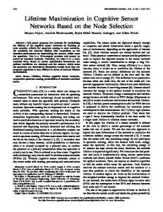
B. Link Scheduling The convex optimization problem (2) is feasible only if the constraints rln ≥ 0, l ∈ Ln , n = 1, . . . , N are feasible. For the approximate rate constraint, these constraints imply that each link has an SINR≥ 1 during the scheduled slots. If we schedule all links during all slots, the problem may be infeasible. There is no simple characterization of the set of link schedules for which the constraints rln ≥ 0, l ∈ Ln , n = 1, . . . , N are feasible. Hence, in order to use problem formulation (2) to compute a transmission scheme corresponding to the best link schedule, we need to solve this problem for all possible link schedules. However, for a network of L links, and for a schedule frame that has N time slots, there are 2N L different link schedules. Hence, the complexity of this approach is doubly exponential in the number of slots and the number of links. This results in a tradeoff between the computational complexity and the quality of the solution. When we compare the solution for say N slots and 2N slots, the solution corresponding to 2N slots gives a network lifetime greater than or equal to the lifetime corresponding to the solution for N slots. This is because we have more freedom in choosing the link schedules, and hence can find a transmission scheme that gives a larger network lifetime. In this paper, we take N to be a system constant. We use a suboptimal approach to iterate between scheduling and computation of rates and powers. The links that carry a larger amount of traffic should be scheduled over a greater number of time slots - this decreases the average transmission power consumption over the links. Hence, the link schedule is adapted to the solution of problem (2) at each iteration, and in turn the convex optimization problem is solved for the new link schedule. Note that we motivate our link adaptation heuristic for a scenario in which transmission power dominates the power consumption in the circuit. This is a realistic scenario for interference-limited networks with high data rates. For a discussion of the tradeoffs between decreasing transmission power and decreasing circuit power, see [5]. The algorithm is illustrated in Fig. 1. Geometrically, the feasible set in problem (2) is a convex subset of the feasible set in problem (1). The heuristic approach proposed below solves a series of convex optimization problems with feasible regions given by different convex subsets of the original optimization problem in (1). Each convex subset corresponds to a link schedule and approximation of the rate constraints by convex constraints.

SUBMITTED TO THE IEEE TRANS. ON WIRELESS COMMUNICATIONS

13

C. Algorithm The iterative approach used to compute an approximate optimal strategy is summarized in the flowchart in Fig. 2. The steps of the algorithm are as follows. 1) Find an initial suboptimal, feasible schedule. A good candidate would be a schedule in which all links are activated at least once in each frame of N slots, and also links that are activated in the same slot interfere only weakly. 2) Solve problem (2) to find an optimal routing flow and transmission powers during each slot for the approximate rate constrant. If the problem is infeasible, quit. 3) Remove l from Ln if

P

Gll Pln Glk Pkn +N0

k∈Ln ,k6=l

≤ γ0 , where γ0 > 1 is a constant close to 1. Since we approximated

the rate as r = log(SINR), links carry little traffic over the slots in which they have an SINR of about 1. P P n ˆ ˆ = arg minn ( k∈Ln ,k6=ˆl Gˆlk Pkn + N0 ). Add ˆl to Lnˆ . If the 4) Find ˆl = arg maxl N n=1 Pl . For this l, find n

resulting schedule is one that was used in a previous iteration, quit. Thus we find a link that consumes the maximum average power over the entire frame and schedule this link to be on during an additional time slot. The selected slot should be the one in which there is minimum interference to this link. If the resulting schedule is one that was used in a previous iteration, quit. 5) Check if

Gll Pln n k∈Ln ,k6=l Glk Pk +N0

P

≥ 1 for all l ∈ Ln and n = 1, . . . , N is feasible. If yes, go to (2), else quit to

prevent an infinite loop. For small networks, we can use a TDMA schedule for step (1). If we assume that the maximum transmission power constraint is loose, the initial schedule is always feasible. However, for larger networks, a TDMA schedule may not be feasible due to the maximum power constraint. In this case, we can use edge coloring on the dual conflict graph [10], where only links which interfere very weakly are allowed be scheduled in the same slot. Note that we can use the gain value Glk as a measure of interference. For example, we can say that a link k is said to interfere with a link l if Glk ≥ α; then the total interference to any link will be bounded by α|V |2 Pmax . For a detailed discussion of this approach, we refer the readers to [10], [9]. The algorithm uses a greedy heuristic to adaptively schedule links at each iteration, and then re-solves the convex optimization problem (2) to determine an optimal routing flow and link transmission powers and rates in each slot.

SUBMITTED TO THE IEEE TRANS. ON WIRELESS COMMUNICATIONS

14

As we will see in the following section, even such a simple greedy heuristic can give strategies with a higher network lifetime than that given by static approaches to scheduling (e.g. TDMA and time sharing between modes in which links separated by a minimum distance are scheduled together). The gains in network lifetime are due to energy-efficient multihop routing, frequency reuse, and load balancing. Also, note that the algorithm will terminate in at most 2N L steps. However, since the solution computed at each step is feasible, we can terminate the algorithm as soon as we have a competitive solution.

IV. N UMERICAL R ESULTS Here we concentrate only on the transmission energy. Thus we take Pct , Pcr = 0. Note that transmission energy dominates at high data rates. We assume Gij =

k , dm ij

where dij is the distance between the transmitter of link j

and the receiver of link i, k is a constant that depends on system parameters such as the carrier frequency and antenna gain [30], and m is the path loss exponent. For the computations that follow, we take m = 4, k = 1, N0 = 1, Ev = 50, ∀v ∈ V . Thus if a transmitter transmits at unit power to a receiver at a distance of 1m, then in

the absence of any interference the receiver SINR is 1. We will compare the performance of our algorithm with that of transmission schemes with specific scheduling at the MAC layer, outlined below. (1) Uniform TDMA: Each link in the network is scheduled for an equal number of time slots. In our computations we consider the number of slots per frame to be a multiple of the number of links. (2) Optimal TDMA: This refers to an optimal TDMA schedule computed by the mixed integer-convex problem formulation in Section II.E. (3) Spatially periodic time sharing: This refers to a link layer scheduling scheme specific to one-dimensional (string and linear) topologies discussed below. A spatially periodic scheme with parameter T refers to a link schedule with T time slots per frame. In each time slot every T th link is activated. Also, every link is activated once in every T slots. Thus if there are N links, in the first slot, links 1, T + 1, 2T + 1, . . . are activated, while in the second slot, links 2, T + 2, 2T + 2, . . . are activated, and so on. For example, T = 2 refers to a scheme which consists of two alternating transmission modes, with each transmission mode consisting of alternate links that are active. Also, the algorithm was initialized with a uniform TDMA link schedule for all the computations that follow.

SUBMITTED TO THE IEEE TRANS. ON WIRELESS COMMUNICATIONS

15

A. String Topology A string topology consists of one source and one sink, connected by intermediate nodes that are arranged linearly. Each pair of neighboring nodes is separated by the same distance d, and connected by a directed link. The network carries information generated by the source to the sink. An example of a string topology is shown in Fig. 3, with s2 , . . . , s9 = 0. Here each link needs to support the same amount of average rate, which is the rate at which the

source generates information. For this topology there is only one routing path from the source to the sink. Hence, we only need to compute the link schedule and transmission powers and rates for each slot. We take d = 1m. Fig. 4(a) shows the network lifetime of a string topology of 10 nodes and 9 links achieved by our algorithm (curve labeled as “alg”), for different source rates. We used a frame length of 18 slots; the algorithm was initialized with a TDMA schedule in which every link was turned on for two time slots in each frame. The figure also shows the network lifetime under the TDMA scheme1 , and under different spatially periodic schedules (curves labeled with corresponding T values). We can see that the algorithm performs well for low source rates, but as the source rate increases, it does increasingly worse compared to the spatially periodic scheme with optimal T . We would like to point out that for a string topology with many nodes, the spatially periodic schedule with optimal value of T will be close to an optimal link schedule. This is because all links carry the same amount of traffic, and the nodes that are not close to either the source or the sink experience similar interference conditions. Hence, we do not need adaptive scheduling, we can use a fixed periodic link schedule with optimal T . The network lifetime as a function of the value of T (for spatially periodic time sharing) is plotted for different source rates in Fig. 4(b). For a given source rate, the network lifetime first increases with T , and then decreases with T , with the optimal lifetime obtained for some value of T between 2 and 9. This illustrates the trade-off between (1) decrease in transmission energy by allowing each node to transmit data at a lower rate in each scheduled time slot and (2) increase in transmission energy due to interference caused by scheduling many links in the same time slot. The uniform TDMA scheme (T=9) performs poorly compared to the optimal spatially periodic schedule. Thus this topology illustrates the advantage of frequency reuse by simultaneous scheduling of links that do not interfere much. 1

Uniform TDMA is an optimal TDMA scheme since each link supports the same data rate over an AWGN channel with same noise

power.

SUBMITTED TO THE IEEE TRANS. ON WIRELESS COMMUNICATIONS

16

B. Linear Topology The linear topology is a simple generalization of the string topology. The nodes are again arranged linearly, but now each node is a source generating data at a possibly different rate. We computed the network lifetime using our algorithm for a linear topology of 10 nodes and 9 links with d = 1m. This topology is shown in Fig. 3. The source rates were taken to be s1 , . . . , s9 = 0.1 nats/Hz/s, while the frame length was N = 18 slots. Fig. 5 shows the best network lifetime achieved until each iteration. We can see that the lifetime increases as the link schedule adapts to the rates and transmission powers computed by solving problem (2). We note that the increase in lifetime is not monotonic. The network lifetimes under different classes of link schedules are as follows. The network lifetime achieved by the best spatially periodic scheme (T = 3) was 12% lower than that achieved by our algorithm. As we can see from Fig. 6, the algorithm provides a greater number of slots to links that carry more traffic, and hence equalizes the average power consumption over the links with the four highest data rates. This is unlike the spatially periodic scheme which allocates the same number of time slots for each link. Also, uniform TDMA (Tnet = 0.14) and optimal TDMA (Tnet = 1.35) perform poorly because they do not take advantage of frequency reuse. However, optimal TDMA is far superior than uniform TDMA because it allocates more slots to links with higher data rates.

C. Rhombus Topology The rhombus topology is shown in Fig. 7(a). The total number of variables in the optimization problem for this network is 192. We use this topology to illustrate the routing behavior of our algorithm. There are four source nodes - nodes 1,2,3,4 with source rates s1 , s2 , s3 , s4 , respectively. Node 5 is the sink node. If we neglect interference and consider only the path loss, the minimum energy routes from the sources to the sink are (1,3,5), (2,3,5), (3,5) and (4,3,5) for sources 1,2,3, and 4, respectively. This topology illustrates the load balancing properties of the algorithm proposed in Section 3. A frame length of 16 time slots was used. The algorithm was initialized with a uniform TDMA schedule, with each link active for two of the 16 time slots in each frame. We used the algorithm to compute an efficient transmission strategy for two different sets of source rates. (1) All sources on: We used our algorithm to compute a transmission strategy for si = 0.4 nats/Hz/s , i = 1, 2, 3, 4. The rates, powers, and the

SUBMITTED TO THE IEEE TRANS. ON WIRELESS COMMUNICATIONS

17

schedule computed by the algorithm are shown in Table I. Link (3,5) carries more traffic than links (1,3), (2,5), and (4,5); also links (1,3), (3,5) have higher gain than the other two links. Hence, link (3,5) is allocated the highest number of slots, followed by links (2,5) and (4,5). We can see that the average power consumption of nodes 2,3,4 is about the same; hence these nodes die out at about the same time. The sources 2 and 4 send all their data directly to the sink rather than use the minimum energy routes; this avoids overloading node 3 with a large amount of data to transmit. (2) Source 2 off: An approximate optimal strategy was recomputed with s2 = 0, si = 0.4 nats/Hz/s , i = 1, 3, 4. The results are shown in Table II . Since node 2 does not generate data, a fraction of the data of node

1 is routed through node 2. Since only a fraction of node 1’s data is routed through node 3, we can route some data of node 4 over the minimum energy route (4,3,5) through node 3. Hence, node 4 uses a multihop path for a fraction of its data. This equalizes the average power consumption of nodes 1,3 and 4. Also, since link (3,5) carries significantly higher data than other links, it is scheduled over more slots than the other links. The value of the network lifetime for the strategy computed at each iteration is shown in Fig. 7(b). We can see from the figure that the network lifetime for the strategy computed by our algorithm is about 4.55 times that for the uniform TDMA schedule (corresponding to the first iteration), when all sources are on. When r2 = 0, the value computed by the algorithm is about 2.57 times that for the uniform TDMA schedule. We can also consider minimum energy routing, with uniform TDMA for links that carry data. The minimum energy routing for this topology would use links (1,3),(2,3),(4,3),(3,5); the bottleneck node is node 3 which needs to transmit data of all the nodes to node 5. The network lifetime in this case is 0.33 when all sources are on, and 4.1 when r2 = 0. The results are summarized in Table III. We can see that optimal TDMA schemes perform very well (in fact better than our algorithm which uses a heuristic for adapting link schedules) for the rhombus topology. This is because each link strongly interferes with all other links in this topology, and hence we should not schedule multiple links in the same time slot. This is unlike a linear or a string topology where a link scheduled at one end does not cause significant interference to a link at the other end of the network. V. C ONCLUSIONS AND F UTURE W ORK We considered the problem of computing transmission powers, rates, and link schedule for an energy-constrained wireless network to jointly maximize the network lifetime. For the special case, where we restricted link schedules

SUBMITTED TO THE IEEE TRANS. ON WIRELESS COMMUNICATIONS

18

to TDMA schemes, we obtained the exact optimal transmission scheme as the solution of a mixed integer-convex optimization problem. For the case of general link schedules, we proposed an iterative algorithm to approximate the optimal solution. Each iteration of the algorithm solved a convex optimization problem, where the feasible region was given by a convex subset of the feasible set in the general problem formulation. The algorithm was found to perform well for the topologies considered in this paper. The numerical studies emphasized the importance of cross-layer design for energy-constrained networks, and illustrated the advantages of multihop routing, load balancing, interference mitigation, and frequency reuse in increasing the network lifetime. Traditional approaches such as TDMA and minimum energy routing were found to perform poorly for certain topologies.

A. Discussion and Future Work The computationally intensive part of the algorithm proposed in Section 3.3 is that of solving the convex optimization problem (2). In this paper, we used the barrier method (see, for example, [29]) to solve this problem. Each iteration of this interior point method involves the minimization of a logarthmic barrier function. For quick convergence that is independent of the coordinates in which we solve the problem, the Newton method was used. The Netwon method involves inverting the Hessian of the logarthmic barrier function – this limits the size of the problems that we can solve in a centralized manner since (1) the complexity of inverting a matrix scales as O(n3 ) and (2) the number of variables grows as O(|V |2 ) with the number of nodes |V |. Hence, we outline a

distributed subgradient algorithm. For this algorithm each iteration consists of solving many smaller problems in parallel instead of solving one big optimization problem. Consider the following optimization problem. µ ¶ ¡ ¢ P n ν Qn l λ min. r − ν + (1 + α)e H(l) T (l) H(l) l∈Ln l s.t.

rln ≥ 0,

Qnl ≤ log(Plmax ),

φ(n) ≤ 0

n Let us denote the solution of this problem for given λ, ν as rln∗ (λ, ν), Qn∗ l (λ, ν), l ∈ L . The k th iteration of the

subgradient algorithm is given by rln = rln∗ (λ(k) , ν (k) ),

(k) (k) Qnl = Qn∗ ), l (λ , ν

³ ´ (k) (k) (k) λ(k+1) = λ − α h (λ , ν ) , k v v v +

q = q ∗ (λ(k) )

νv(k+1) = νv(k) − αk fv (λ(k) , ν (k) )

SUBMITTED TO THE IEEE TRANS. ON WIRELESS COMMUNICATIONS

19

³ ´ P where q ∗ (λ(k) ) = arg minq q 2 − qN v∈V λv Ev , and hv , fv are given by (suppressing the dependence on λ, ν ) N X

hv =

X

Qn∗ l

(1 + α)e

∗

− N q Ev ,

fv =

n=1 l∈O(v)∩Ln

N µ X n=1

X

l∈O(v)∩Ln

rln∗

−

X

¶ rln∗

− N sv

l∈I(v)∩Ln

for i ∈ V . Here αk is a positive scalar step size. It can be shown that the iterates converge to the solution of problem (1) if αk → 0,

P∞

k=1 αk

= ∞ (see, for example, [31]). Investigation of thumb rules for choosing the

coordinates to solve the problem, choice of the step size rule, and investigation of the convergence rate are some of the issues that need attention in order to make the algorithm scale for large networks. In order to obtain a globally optimal cross-layer transmission scheme, we need to solve the non-convex problem (1). Obtaining bounds will give us not only the range of attainable globally optimal network lifetimes, but can also serve as a benchmark for our algorithm and other methods in the literature. We can use a branch and bound method, where the lower bounds are given by relaxations and the upper bounds are given by the dual problem. However, since the problem is non-convex and has variables with continuous domains, designing the branching rule and the relaxations is a complicated task; this investigation is an emphasis of our current work. Approximations in [32] seem to be promising for work in this direction. Our framework can easily be adapted to many different algorithms for adapting the link schedule to the corresponding routing and physical layer transmission scheme. Investigation of different link adaptation algorithms as well as solving the optimization problem for more general definitions of network lifetime are other possibilities for interesting future research directions.

R EFERENCES [1] V. Rodoplu and T. H. Meng, “Minimum energy mobile wireless networks,” IEEE J. Selected Areas in Communications, vol. 17, no. 8, pp. 1333–1344, 1999. [2] L. Li and J. Y. Halpern, “Minimum energy mobile wireless networks revisited,” IEEE International Conference on Communications (ICC), 2001. [3] J.-H. Chang and L. Tassiulas, “Energy conserving routing in wireless ad-hoc networks,” Proc. IEEE INFOCOM, pp. 22–31, 2000. [4] R. L. Cruz and A. V. Santhanam, “Optimal routing, link scheduling and power control in multi-hop wireless networks,” IEEE INFOCOM, 2003. [5] S. Cui, A. J. Goldsmith, and A. Bahai, “Energy-constrained modulation optimization,” IEEE Transactions on Wireless Communications, vol. 4, no. 5, pp. 2349–2360.

SUBMITTED TO THE IEEE TRANS. ON WIRELESS COMMUNICATIONS

20

[6] S. Toumpis and A. J. Goldsmith, “Capacity regions for wireless ad hoc networks,” IEEE Transactions on Wireless Communications, vol. 4, pp. 736–748, 2003. [7] D. O’Neill, D. Julian, and S. Boyd, “Seeking Foschini’s genie: optimal rates and powers in wireless networks,” Accepted for publication in IEEE Transactions on Vehicular Technology, 2004. [8] M. Johansson and L. Xiao, “Scheduling, routing and power allocation for fairness in wireless networks,” IEEE Vehicular Technology Conference, 2004. [9] M. Kodialam and T. Nandagopal, “Characterizing achievable rates in multi-hop wireless networks: The joint routing and scheduling problem,” MobiCom, 2003. [10] K. Jain, J. Padhye, V. N. Padmanabhan, and L. Qiu, “Impact of interference on multi-hop wireless network performance,” MobiCom, 2003. [11] B. Radunovic and J. Y. L. Boudec, “Joint scheduling, power control and routing in symmetric, one-dimensional, multi-hop wireless networks,” Modeling and Optimization in Mobile, Ad Hoc and Wireless Networks (WiOpt), 2003. [12] A. J. Goldsmith and S. W. Wicker, “Design challenges for energy-constrained ad hoc wireless networks,” IEEE Wireless Communications Magazine, 2002. [13] U. C. Kozat, I. Koutsopoulos, and L. Tassiulas, “A framework for cross-layer design of energy-efficient communication with QoS provisioning in multi-hop wireless networks,” INFOCOM, 2004. [14] N. Bambos, “Toward power-sensitive network architectures in wireless communications: Concepts, issues and design aspects,” IEEE Personal Communications Magazine, 1998. [15] S. Cui, A. J. Goldsmith, and A. Bahai, “Joint modulation and multiple access optimization under energy constraints,” GLOBECOM, 2004. [16] G. Zussman and A. Segall, “Energy efficient routing in ad hoc disaster recovery networks,” INFOCOM, 2003. [17] A. Sankar and Z. Liu, “Maximum lifetime routing in wireless ad-hoc networks,” INFOCOM, 2004. [18] R. Madan and S. Lall, “Distributed algorithms for maximum lifetime routing in wireless sensor networks,” To appear in the IEEE Transactions on Wireless Communications. [19] T. ElBatt and A. Ephremides, “Joint scheduling and power control for wireless ad hoc networks,” IEEE Transactions on Wireless Communications, vol. 1, pp. 74–85, 2004. [20] S. Cui, R. Madan, A. J. Goldsmith, and S. Lall, “Cross-layer energy miminization in sensor networks,” Allerton Conference on Communication, Control and Computing, 2004. [21] R. Bhatia and M. Kodialam, “On power efficient communication over multi-hop wireless networks: Joint routing, scheduling and power control,” INFOCOM, 2004. [22] M. Johansson, L. Xiao, and S. Boyd, “Simultaneous routing and resource allocation in cdma wireless data networks,” ICC, 203. [23] S. H. A. Ahmad, A. Jovicic, and P. Viswanath, “Upper bounds to generalized transport capacity of wireless networks,” To appear in IEEE Transactions on Information Theory.

SUBMITTED TO THE IEEE TRANS. ON WIRELESS COMMUNICATIONS

21

[24] G. J. Foschini and J. Salz, “Digital communications over fading radio channels,” Bell Systems Technical Journal, pp. 429–456, 1983. [25] T. H. Lee, The Design of CMOS Radio-Frequency Integrated Circuits. Cambridge University Press, 1998. [26] V. Balakrishnan, S. Boyd, and S. Balemi, “Branch and bound algorithm for computing the minimum stability degree of parameterdependent linear systems,” Int. J. of Robust and Nonlinear Control, vol. 1, pp. 295–317, 1991. [27] E. L. Lawler and D. Wood, “Branch-and-bound methods: A survey,” Operations Research, vol. 14, pp. 699–719, 1966. [28] D. O’Neill, D. Julian, and S. Boyd, “Adaptive management of network resources,” IEEE Vehicular Technology Conference, 2003. [29] S. Boyd and L. Vandenberge, Convex Optimization. Cambridge University Press, 2003. [30] A. J. Goldsmith, Wireless Communications. Cambridge University Press, 2005. [31] N. Z. Shor, Minimization Methods for Non-differentiable Functions. Springer-Verlag, 1985. [32] J. Papandriopoulos, S. Dey, and J. S. Evans, “Distributed cross-layer design of MANETs in composite fading through global optimization,” Submitted to the IEEE Journal on Selected Areas in Communications (Special Issue on Non-Linear Optimization).

SUBMITTED TO THE IEEE TRANS. ON WIRELESS COMMUNICATIONS

22

Feasible set for appr. rate constraint and fixed link schedule

Feasible Set

Fig. 1. Algorithm - Solving a series of approximate convex optimization problems

Initialize with feasible suboptimal schedule

Compute optimal rates, powers

YES

Feasible? NO YES

SINR>1 feasible?

Turn off links with SINR appr. 1 NO NO

Allocate an additional slot to a link with the max. avg. power

Repeated schedule?

YES Quit

Fig. 2. Iterative approach to compute powers, rates and link schedule.

SUBMITTED TO THE IEEE TRANS. ON WIRELESS COMMUNICATIONS

s1

23

s2

s9

L1

L2

1

L8

sink

L9

2

9

10

d

Fig. 3. Linear Topology

90

100

T=2 T=3 T=4 TDMA alg

80

80 70

network lifetime

60 50 40 30

50 40

20

10 0

s=0.2 s=0.3 s=0.4 s=0.5 s=0.6

60

30

20

10

0.2

0.3

0.4

0.5

0.6

0

0.7

2

3

4

source rate (nats/Hz/s)

5

6

7

T

(a) Lifetime as a function of rate

(b) Spatially Periodic Schedules Fig. 4. String Topology Lifetimes

12

10

network lifetime

network lifetime

70

90

8

6 alg uniform TDMA optimal TDMA T=3 spatially periodic

4

2

0 0

5

10

15

20

25

iteration number

Fig. 5. Linear Topology - Network lifetime

8

9

10

SUBMITTED TO THE IEEE TRANS. ON WIRELESS COMMUNICATIONS

24

7

5 4.5

6

avg. power consumption

no. of slots allocated

4

5

4

3

2

3.5 3 2.5 2 1.5 1

1 0.5

0

1

2

3

4

5

6

7

8

0

9

1

2

3

4

5

link

6

7

8

9

link

(a) number of slots per frame for links L1 , . . . , L9

(b) avg. power consumptions on links L1 , . . . , L9

Fig. 6. Transmission Scheme for a Linear Topology - average rate over link i is 0.1i nats/s/Hz.

s2 2

20 (1,1)

all sources on source 2 off

18 16

s1 network lifetime

14

sink 1

3

5 (2,0)

(1,0)

(0,0)

s3

12 10 8 6 4

4

2

(1,−1)

0 0

2

s4

4

6

8

iteration number

(a) Topology

(b) Lifetime Computation Fig. 7. Rhombus Topology

link

no. of slots

avg. rate

avg. power

(1,3)

2

0.4

3.06

(3,5)

5

0.8

4.81

(2,5)

4

0.4

4.95

(4,5)

4

0.4

4.95

TABLE I R HOMBUS T OPOLOGY - si = 0.4, i = 1, 2, 3, 4.

10

SUBMITTED TO THE IEEE TRANS. ON WIRELESS COMMUNICATIONS

link

25

no. of slots

avg. rate

avg. power

(1,2)

2

0.2

2.52

(1,3)

2

0.2

0.61

(2,5)

2

0.2

2.94

(3,5)

7

0.8

3.13

(4,3)

2

0.2

0.61

(4,5)

2

0.2

2.52

TABLE II R HOMBUS T OPOLOGY - s2 = 0, si = 0.4 NATS /H Z / S , i = 1, 3, 4.

Tnet

Tnet

s2 = 0.4

s2 = 0

Uniform TDMA

2.22

6.22

Optimal TDMA

11.23

16.96

Algorithm

10.10

16.00

0.33

4.1

Transmission Scheme

Uniform TDMA, min. energy TABLE III

R HOMBUS T OPOLOGY - N ETWORK LIFETIME UNDER DIFFERENT CLASSES OF TRANSMISSION SCHEMES (s1 , s3 , s4 = 0.4 FOR BOTH CASES ).