We use the grid-quorum system [25] as the underlying MAC layer to support power ... The goal is to support continuous queries in an energy-efficient manner.
Cross-Layer, Energy-efficient Design for Supporting Continuous Queries in Wireless Sensor Networks: A Quorum-Based Approach Chia-Hung Tsai, Tsu-Wen Hsu, Meng-Shiuan Pan, and Yu-Chee Tseng Department of Computer Science National Chiao Tung University Hsin-Chu, 30050, Taiwan Email:{chiahung, tsuwen, mspan, yctseng}@cs.nctu.edu.tw Abstract Power saving and query processing are two major concerns in a wireless sensor network. Each of these two issues has been intensively studied separately in the literature. In this work, we are interested in linking the asynchronous power-saving protocol and the continuous query-processing problem together. A cross-layer solution is proposed. On the MAC layer, we propose to use the grid-quorum system [25] to serve as the underlying power-saving framework. On the network layer, we propose to find query paths based on the power cost incurred by grid quorums used by nodes along a path. We show how these two layers interwork with each other to support continuous queries in an energy-efficient way.
Keywords: power saving, protocol design, query processing, routing, wireless sensor network.
1 Introduction The rapid progress of wireless communication and MEMS technology have made wireless sensor networks (WSNs) possible. A WSN normally consists of many inexpensive wireless sensor nodes. Each node is capable of collecting, storing, processing environmental information, and communicating with neighbor nodes. Recently, a lot of research works have been dedicated to WSNs, such as routing [6][9], self-organization [12][23], deployment 1
[8][16][28], and localization [5][20]. Applications of WSNs include emergency guiding [13][26], light control [17][18], and environment monitoring [24]. Power saving and query processing are two main issues in WSNs. Many power-saving MAC protocols have been proposed. In SMAC [30], nodes periodically switch to sleep mode. In PMAC [31], sensors are allowed to adaptively determine their sleep schedules by considering neighbors’ traffic patterns. In RMAC [3], sensor nodes periodically wake up and use their active periods to establish routing paths. Nodes not located on any routing path can go to sleep; otherwise, they have to remain active. GAF [29] divides the network area into square grids. Although sensors can switch between sleep mode and active mode periodically, it guarantees that at least one node per grid remains active to exchange packets with neighboring grids. Span [2] adaptively elects some nodes to stay in active mode and serves as the network backbone. Other nodes periodically check with backbone nodes to see if they need to wake up. Both [2] and [29] may have some redundant sensors to stay active. TAP [7] considers traffic flows and identifies redundant nodes that can go to sleep when establishing routing paths. Most of these schemes require nodes to be synchronized in time, which is costly. Recently, some power-saving protocols have been proposed without requiring time synchronization [1][11][14][25]. On the other hand, query processing in WSNs has also attracted a lot of attention. Directed diffusion [10] achieves energy efficiency by selecting empirically good paths and by caching and processing data inside the network. In [19], data-centric storage is proposed by adopting geographic hashing to offer high data availability and load distribution. TAG [15] is a tiny data service that can significantly reduce bandwidth consumption. A semistructure approach which uses multiple shortest-path trees is proposed in [4] to support scalable data aggregation. A lot of works [21][22] utilize the spatio-temporal correlations of sensing data to achieve energy efficiency. A generic two-tier storage strategy for answering precision-constrained approximate queries is proposed in [27]. Although most of these query-processing works focus on achieving energy efficiency, they all do not specifically address the underlying wake-up/sleep schedules of sensor nodes. In this work, we are interested in applying the quorum-based power-saving protocols
2
[1][11][14][25], which have the advantage of not relying on any time synchronization among sensor nodes, to the continuous query-processing problem. A continuous query involves sending periodical reports from a source to a sink and is commonly seen in WSNs. More specifically, we will adopt the grid-quorum system [25] to derive the wake-up/sleep schedules of sensor nodes. Multiple query paths may coexist, each with its preferred grid quorum. We will show how these paths (and thus grid quorums) interact with each other to meet each query’s bandwidth requirement in an energy-efficient way. Although global clock synchronization is not necessary, we will suggest to employ an optional local slot synchronization to improve nodes’ energy efficiency. Compared to existing works, this paper contributes in proposing a cross-layer approach to integrating the grid-quorum system with continuous queries. Simulation results are presented to evaluate our results. The rest of this paper is organized as follows. Section 2 presents our cross-layer system architecture. The detail MAC layer (quorum layer) and network layer (query-processing layer) are presented in Section 3 and Section 4, respectively. Section 5 contains our simulation results. Finally, Section 6 concludes this paper.
2 System Architecture We are given a WSN for supporting continuous queries. A continuous query is a unicast with sensing data being periodically delivered from a source node to a sink node. A continuous query, or simply query, is denoted by a 5-tuple (sn , sr , t, p, len), where sn is the sink node, sr is the source node, t is the lifetime of the query, p is the period that sr will generate reports, and len is the expected packet length per report. Multiple queries may coexist in the network. We use the grid-quorum system [25] as the underlying MAC layer to support power management and develop a routing layer on the top of the quorum system to determine its parameters. The goal is to support continuous queries in an energy-efficient manner. We propose a 2-layer architecture as shown in Fig. 1. When a continuous query arrives at the network layer, the sink will broadcast a query request (QREQ) packet to find a reporting path to the source. Such QREQ packets will be flooded around the network. To reply, the source will unicast a query reply (QREP) packet to the sink. To save sensor nodes’ energy, 3
Query Request/Remove
DSR-like Routing
Network Layer
QREQ/QREP/QREM
QSI Table
Quorum adjustment command
Grid-Quorum System
MAC Layer
Quorum Set
Power mode command
PHY layer
Figure 1: The proposed 2-layer architecture.
a cost function is designed at the network layer to select query paths and to dynamically choose/adjust the quorum system’s parameters. Then, the MAC layer will give power mode commands to the underlying layer. Note that when there are multiple queries, our cross-layer approach will try to increase the overlapping among nodes’ quorums to reduce the energy costs to support these queries. After a query expires, a query remove (QREM) packet will be sent along its query path. Each node will maintain a Query Session Information (QSI) table to keep track of the query paths that currently pass it and the quorums to support these paths. Table 1 shows the structure of the QSI table. Gird quorums in this table will together form the quorum set of the node. The detail MAC-layer and network-layer operations will be discussed in Section 3 and Section 4, respectively.
4
Table 1: An example of the QSI table. Query Up Node (31, 99, 2000, 40, 100) 55 (101, 29, 1000, 20, 100) 63
Down Node 129 129
Quorum (8, 5, {1}, {1}) (5, 4, {3}, {3})
Additional Quorum φ φ
g1 = (4, 3, {1},{1})
(a)
1
2
3
4
5
6
7
8
9 10 11 12
1 2 3 4 5 6 7 8 9 10 11 12 1 2 3 4 5 6 7 time
g2 = (4, 4, {1,2},{1})
(b)
1
2
3
4
5
6
7
8
9 10 11 12
1 2 3 4 5 6 7 8 9 10 11 12 13 14 15 16 1 2 3 time
13 14 15 16 G(v) = {g1, g2}
(c)
1
2
3
4
5
6
7
8
9 10 11 12
1
2
3
4
5
6
7
8
9 10 11 12
1 2 3 4 5 6 7 8 9 10 11 12 13 14 15 16 17 18 19 time
13 14 15 16 Κquorum slot (active) Κnon-quorum slot (sleep)
Figure 2: An example of a quorum set.
5
3 Quorum Layer 3.1 Grid Quorum System Power-saving protocols for wireless networks need to ensure that nodes’ wakeup patterns will overlap with their neighbors’ patterns for communication opportunity. It is pointed out in [25] that two major challenges that one would encounter when designing a power-saving protocol are: clock synchronization and neighbor discovery. Therefore, many solutions try to enforce nodes to synchronize their clocks. However, time synchronization in a large-scale distributed environment is very costly. An alternative is to develop asynchronous powersaving protocols. The quorum-based protocols [1][11][14][25] are such solutions. Basically, they require nodes to wake up and sleep based on some pre-configured rules, but nodes do not need to synchronize their clocks. Several kinds of quorums have been proposed, such as tree quorums and grid quorums. In this work, we will adopt the grid-quorum system [25] as our power-saving mechanism. Fig. 2(a) shows a grid-quorum example. Each node’s time axis is divided into repetitive n1 × n2 time slots, which are called a group. In each group, its slots are arranged as an n1 × n2 array in a row-major manner. From the array, the node can arbitrarily pick one column and one row of slots as its wakeup slots, or called quorum slots. Each node must stay awake in quorum slots, and can go to sleep in the remaining n1 × n2 − n1 − n2 + 1 slots. Note that nodes’ clocks do not need to be synchronized. The concept has been applied to IEEE 802.11-based ad hoc networks in [25] by enforcing all nodes to take the same values of n1 and n2 . In [1], it is further shown that even if two nodes use different n1 and n2 , transmission opportunity (i.e., overlapping of wake-up patterns) between them is still guaranteed.
3.2 Quorum Set for Continuous Queries In this work, we are interested in applying the grid-quorum system to support continuous queries in a WSN. The wake-up/sleep schedule of a node will be determined by one or multiple grid quorums, which we call quorum set. The quorum set of a node v is denoted
6
by G(v). Each grid quorum is denoted by a 4-tuple g = (n1 , n2 , R, C), where n1 and n2 are the numbers of rows and columns, respectively, of the grid array, R is a set of rows, and C is a set of columns. Note that this is an extension of the original definition in [25] since all entries falling in rows of R or columns of C are quorum slots. We define the duty cycle of a grid quorum g = (n1 , n2 , R, C) by dty(g) =
|R| × n1 + |C| × n2 − |R| × |C| . n1 × n2
(1)
For example, Fig. 2(a) shows a grid quorum g1 following the original definition of [25] (it contains only one row and one column of quorum slots). In Fig. 2(b), g2 = (4, 4, {1, 2}, {1}) is an extended grid quorum, which contains two rows and one column of quorum slots. Fig. 2(c) shows a quorum set G(v) = {g1 , g2 }, in which case, v will run both quorums g1 and g2 simultaneously by “OR” the quorum slots of both g1 and g2 . That is, whenever any of the grid quorums in G(v) indicates that a slot is a quorum slot, v will enter the active mode. So Fig. 2(c) is the “OR” of the two sequences in Fig. 2(a) and Fig. 2(b).
4 Query-Processing Layer In our system, when a node does not support any continuous query, its quorum set will contain only one default grid quorum gdef with minimum duty cycle. As more and more continuous queries (query paths) pass the node, its quorum set will contain more grid quorums. The default quorum is defined as gdef = (nmax , nmax , {rnd}, {rnd}), where nmax is a large number and rnd is a random integer between 1 and nmax . A DSR-like routing protocol will be applied. To select a routing path, an energy cost function will be defined to evaluate the quality of a query path. Basically, a new path will try to increase its overlapping of quorum slots with existing paths’ quorum slots while maintain sufficient communication capacity. Section 4.1 presents the query-requesting process, followed by the query-replying and the query-removing processes in Section 4.2 and Section 4.3. Finally, in Section 4.4, a lightweight local slot synchronization is proposed to increase energy efficiency.
7
4.1 Query-Requesting Process This part contains three modules, quorum preparing, QREQ initiating and processing, and QREQ rebroadcasting, as explained below. A) Quorum Preparing: When a sink node sn has a query y = (sn , sr , t, p, len) to a source node sr , it will compute a grid quorum gini to support the query y as follows. Here we assume that from past history, the length len per report is already known. 1. Compute a pair (n1 , n2 ) such that n1 × n2 ≈ p and n1 is as close to n2 as possible. 2. Construct a grid quorum gini = (n1 , n2 , R, C), where R/C contains a random row/column. 3. Then we check whether dty(gini) ≥
len r
·
1 p
holds, where r is the transmission rate of
a node. If so, we will adopt gini as the grid quorum to serve the query y. Otherwise, we will continuously add rows or columns to R or C to increase the duty cycle value dty(gini), until dty(gini) ≥
len r
·
1 p
holds.
Note that gini is only considered as a candidate to support y; it may or may not be actually used on the query path between sr and sn . This will become clear later. B) QREQ Initiating and Processing: There are two cases involving in producing a QREQ packet: (i) a node initiates a new query and (ii) a node receives a QREQ and rebroadcasts it. Below, we will only consider case (ii) and regard case (i) as a special case of case (ii). So we suppose that node xi receives from node xi−1 a QREQ(gini , y, c, P AT H) for possibly supporting a query y initiated by node x0 , where gini is the grid quorum computed by x0 (by the above step A), c is the cost calculated by xi−1 , and P AT H is a list of 2-tuples, where each 2-tuple is of the form (node id, quorum). Note that P AT H contains the nodes that the QREQ has traversed so far and the grid quorums chosen by them. In case that xi is the query initiator (i.e., x0 = xi ), we will imagine that a virtual QREQ is sent by xi to itself such that c = 0 and P AT H = () is an empty list. On receipt such a QREQ, the following discusses how xi rebroadcasts this QREQ. First, xi will find a quorum to serve query y, which we call gser (y). If xi is not currently passed by any query path, it will set gser (y) = gini . Otherwise, xi will try to pick an existing 8
quorum in its quorum set G(xi ) or adopt gini to serve y. It will try to pick an existing one in G(xi ) first. Recall the definition of duty cycle in Eq. (1). Given G(xi ), we can estimate xi ’s duty cycle as follows: Y
DT Y (G(xi )) = 1 −
(1 − dty(g)).
(2)
g∈G(xi )
Also, from xi ’s QSI, we can measure xi ’s current traffic load as follows. For each query z, in xi ’s QSI, its load can be calculated by ld(z) =
len(z) r
·
1 , p(z)
where len(z) is the length of
each sensing report and p(z) is the period per report for query z. So xi ’s current traffic load is X
LD(xi ) =
ld(z).
(3)
∀z∈QSI of xi
Then, xi can measure whether its current quorum set can accommodate y or not by checking LD(xi ) + ld(y) ≤ DT Y (G(xi )). If so, xi will try to pick a candidate quorum gcan ∈ G(xi ) with sufficient capacity to serve y. The capacity of gcan is defined as follows: P 1 Cap(gcan ) =
sj ∈QS(gcan ) s-deg(sj )
n1 (gcan ) × n2 (gcan )
,
(4)
where n1 (gcan ) and n2 (gcan ) are the numbers of rows and columns of gcan , respectively, QS(gcan ) means the set of quorum slots of gcan , and s-deg(sj ) is the share degree of the quorum slot sj in gcan . Here the share degree of sj is the estimated average number of quorums which will also regard slot sj as a quorum slot. This is due to the fact that xi may be running several quorums simultaneously to support multiple query paths, so quorum gcan can only have an equal share of that slot. (For example, in Fig. 2, the share degree of slot 5 of g2 is two and the share degree of slot 6 of g2 is one.) If there exists one gcan such that X
Cap(gcan ) ≥ ld(y) +
ld(z),
(5)
z supported by gcan
then gcan will be assigned to support y and we will set gser (y) = gcan . Otherwise, no existing quorum in G(xi ) can support y and we will check the following two conditions to see if it is possible to include gini into G(xi ): 9
• DT Y (G(xi ) ∪ {gini }) ≥ LD(xi ) + ld(y) • Cap(gini) ≥ ld(y) If both conditions are met, we will set gser (y) = gini ; otherwise, this query is beyond the capacity of xi to be supported and the QREQ will be discarded. Finally, if y can be supported, xi will append the 2-tuple (xi , gser (y)) to the list P AT H and proceed to the next step. The above steps have determined the quorum gser (y) to support y. Next, we will compute the additional energy cost to support y. There are two costs associated with this: (i) the average extra energy cost Cact for xi to remain active per slot and (ii) the average extra energy cost Ctx for xi to transmit data for y per slot. For (i), recall that gser (y) is the quorum ′ to serve y by xi . Let gser (y) be the quorum selected by xi−1 to serve y. We will actually ′ enforce xi to include gser (y) into its quorum set, so that xi can smoothly transmit data to
xi−1 . The cost Cact is defined as ′ Cact = Eact × (DT Y (G(xi ) ∪ {gser (y), gser (y)}) − DT Y (G(xi ))),
where Eact is the energy to remain active for one full slot. This means the extra amount of energy for xi to remain active per slot in order to support y. For (ii), the cost Ctx is defined as Ctx = (Etx − Eact ) ×
len(y) 1 × , r p(y)
where Etx is the energy to transmit one full slot of data. The total addition energy cost for xi to support y is Cact + Ctx . So we will set c = c + Cact + Ctx . C) QREQ Rebroadcasting: The above steps have determined the new c and P AT H if xi decides to support y. Node xi will also maintain the minimum cost cmin for all paths from x0 to xi that xi has learned so far. If cmin ≥ c, then xi will rebroadcast QREQ(gini , y, c, P AT H) containing the new c and P AT H and set cmin = c. Note that in cast that xi is the source sr , rebroadcasting QREQ is not necessary (this will be discussed in Section 4.2).
10
4.2 Query-Replying Process When a node xi receives from xi−1 a QREQ(gini , y, c, P AT H) initiated by a node x0 and finds that it is the sink node of the query y, it will prepare to periodically report its sensing data to x0 according to the parameters specified in the query. Node xi will collect QREQs for a while and choose the QREQ(gini , y, c, P AT H) with the lowest cost c. Then xi will unicast QREP(y, P AT H) back to x0 . The QREP will sequentially traverse nodes along the reverse direction of P AT H. For each node xj receiving the QREP, it can identify its serving quorum gser (y) recorded in the P AT H. There are two cases: • If G(xj ) = {gdef }, xj will directly set G(xj ) = {gser (y)}. • Otherwise, xj will set G(xj ) = G(xj ) ∪ {gser (y)}. ′ Also, xj can find the serving quorum, say gser (y), picked by its previous node in P AT H. If ′ ′ gser (y) 6= gser (y), xj will further set G(xj ) = G(xj ) ∪ {gser (y)}. This is for xj to cooperate
with its previous node so as to smoothly transmit its data to its previous node. Finally, xj will adjust its QSI table as follows (refer to Table 1). A new entry will be added such that Query = y, Up Node = xj ’s previous node, Down Node = xj ’s next node, Quorum = gser (y), ′ and Additional Quorum = gser (y).
After a node adjusts its quorum set, it can wake up and sleep according to the quorums in its set. Quorums do not need to synchronize with each other. Whenever any quorum in its set enters a quorum slot, the node has to be active in that slot. Also note that when a quorum slot belongs to multiple queries, the transmission opportunity should be equally shared by all these queries.
4.3 Query-Removing Process When a query session y terminates, the sink node can identify this fact by checking its QSI table. Then it can initiate a QREM(y) packet along the query path to the sink. Each intermediate node when receiving the QREM(y) will remove the corresponding entry from its
11
QSI table. Also, the corresponding quorums to support will be removed from their quorum slots. Again, each node will wake up and sleep according to its new quorum slots.
4.4 Local Slot Synchronization Although the quorum system can guarantee the communication opportunity of any two asynchronous nodes, in this section we will suggest a lightweight local slot synchronization to improve energy efficiency and reduce transmission delays of sensing reports. Here, we only propose to synchronize local nodes’ slots and local nodes’ quorums. We summarize our rules as follows: • At the clock level, two neighboring nodes will try to synchronize their clocks by aligning their slots. That is, they will try to synchronize the beginning of slots at each side. • At the quorum level, if two neighboring nodes use the same quorum in their quorum sets, they will try to synchronize this quorum by aligning the first slot of this quorum at each side. (Different quorums of these two nodes do not need to be synchronized. Similarly, inside each node, two different quorums do not need to be synchronized). The above two rules do not address how to break the tie when a node has multiple neighbors and/or when a node shares the same quorum with multiple neighbors. We propose to assign priority by the following rules: • Along a query path, a node that is closer to the source node has a higher priority. • Between two query paths, the path which was established earlier (i.e., with an earlier timestamp) has a higher priority.
5 Simulation Results 5.1 Simulation Environments Since large-scare deployment is difficult to realize, we develop a simulation environment to verify the energy efficiency factor of our cross-layer query-processing protocol. We set up 12
a 400 × 400 m2 sensing field, on which hundreds of sensor nodes are randomly deployed. The transmission range and carrier sensing range of each sensor node are set to 50 and 100 meters, respectively. In our simulations, we will randomly generate several sink-source continuous query pairs with random report periods and lifetimes. The whole simulation time is 7200 seconds. To evaluate the energy consumption, the power consumption rates of a wireless interface are set to 50, 50, 45, and 5 mW under transmit, receive, idle, sleep modes, respectively. The default quorum gdef is set to (40, 40, {1}, {1}) with each quorum slot fixed to 0.1 second. Hence, each node will initially operate under 5% duty cycle and each quorum group is 160 seconds. Fig. 3 shows a scenario of our system which runs 4 continuous queries simultaneously. It shows that there exists path sharing between the sink-source pairs (y1 , y1′ ) and (y3 , y3′ ) from node 8 to node 131, and the sink-source pairs (y2 , y2′ ) and (y4 , y4′ ) from node 148 to node 24. After the simulation terminates, the percentage of nodes’ residual energy is displayed in Fig. 4. In the following sections, we will discuss the benefit of our cross-layer design and the impact of query loads on our approach.
5.2 Impact of Our Cross-Layer Design To verify the benefit gained from our cross-layer design, we will compare our approach against two schemes. Both schemes apply shortest path routing. The first one lets each query path adjust its quorum on this own, but there is no coordination between paths’ quorums; this scheme is referred to as SP-NC (shortest-path, no-coordination). The second one enforces all quorum paths to share the same quorum; this scheme is referred to SP-GQ (shortest path, global-quorum). We show our results below. A) Comparison with the SP-NC Scheme: Each query reporting period is set to 60 seconds. Query requests are randomly injected at a rate of one query per 500 seconds. Fig. 5 shows the minimal residual energy among all nodes. Since our scheme encourages a new path to overlap with existing paths, it shows that the SP-NC scheme is more likely to exhaust some particular nodes’ energy.
13
Figure 3: A path-sharing scenario.
Residual Energy
49.5 49
49.5
48.5
49 48.5
48
48
47.5
47.5
47
47 400 350 300 0
250 50
100
200 150
150 200
250
100 300
350
50 4000
Figure 4: A scenario of the percentage of nodes’ residual energy after executing 4 continuous queries.
14
Min Residual Energy
50
Our approach SP-NC
45
40
35
30 100
200
300
400 500 600 Number of Nodes
700
800
900
Figure 5: Comparison to the SP-NC scheme on minimal residual energy.
50
Residual Energy
45 40 35 30 25 20 400
Average Residual Energy, SP-GQ Min Residual Energy, ours Average Residual Energy, ours 500
600 700 800 900 Query Generation Period(s)
1000
1100
Figure 6: Comparison to the SP-GQ scheme on nodes’ residual energy.
15
70
r = 250kbps r = 100kbps r = 50kbps r = 10kbps
65 60 55 50 45 40 35 30 100
r = 250kbps r = 100kbps r = 50kbps r = 10kbps
65 Min Residual Energy
Average Residual Energy(%)
70
60 55 50 45 40 35
200
300
400
500
600
700
800
30 100
900
200
300
Number of Nodes
600
700
800
900
800
900
(b)
70
70
r = 250kbps r = 100kbps r = 50kbps
65
r = 250kbps r = 100kbps r = 50kbps
65
60
Min Residual Energy
Average Residual Energy(%)
500
Number of Nodes
(a)
55 50 45 40 35 30 100
400
60 55 50 45 40 35
200
300
400
500
600
700
800
900
Number of Nodes
30 100
200
300
400
500
600
700
Number of Nodes
(c)
(d)
Figure 7: The energy consumption of our system under different transmission rates (r). B) Comparison with SP-GQ scheme: The SP-GQ scheme will pick the quorum with the lowest duty cycle that can meet all nodes’ requirement as the global quorum. On the contrary, our scheme can dynamically adjust each query path’s quorum. The results are in Fig. 6. We fix the number of nodes to 200 and set the query generation rate to one query per 500 seconds to 1000 seconds. It shows that our cross-layer design can result in much higher average residual energy. Even the minimum residual energy of our scheme still significantly outperforms that of SP-GQ. Also, the query generation rate has little impact on the energy consumption of our scheme.
16
5.3 Impact of Traffic Loads Recall the query load estimation in Section 4.1. It can be influenced by three factors: transmission rate, packet length per report, and reporting period. In the following, we will discuss the impact of traffic loads on energy consumption. A) Impact of Transmission Rate: A smaller transmission rate r will result in slower transmission (and thus a higher traffic load). Hence, we evaluate the energy consumption of our system by varying the transmission rate at 250 kbps, 100 kbps, 50 kbps, and 10kbps. In Fig. 7(a)-(b), we randomly inject queries at a rate of one query per 100 seconds. In Fig. 7(c)(d), we randomly inject queries at a rate of three queries per 1000 seconds. Each report is 100 bytes. We can see that a lower r might incur higher energy consumption. In Fig. 7(a) and Fig. 7(c), we see that both transmission rate and number of nodes make little impact on the average residual energy because our protocol only causes nodes on query paths to increase their duty cycles. All other nodes still operate with the default quorum. However, if we look at the node with the minimal residual energy, there do exist some differences, as shown in Fig. 7(b) and Fig. 7(d). A lower r will cause some nodes to consume more energy than others but the impact is still quite smaller. B) Impact of Packet Length: Here, we vary the length len per report to evaluate the energy performance of our scheme. The transmission rate r is fixed to 250 kbps and len varies from 100, 1000, to 5000 bytes. Similar with the previous case, the query generation rates are one and three queries per 1000 seconds in Fig. 8(a)-(b) and Fig. 8(c)-(d), respectively. Fig. 8(a) and Fig. 8(c) show that the average residual energy under different lens, while Fig. 8(b) and Fig. 8(d) show the minimal residual energy under different lens. The tread is generally the same as that in Fig. 7. C) Impact of Query Period: In this scenario, we set r = 250 kbps and len = 100 bytes and vary the reporting period p from 30 to 70 seconds. The query generation rates remain the same with the previous two experiments. The results are similar to the previous cases. As Fig. 9 shows, a higher reporting period will incur less energy consumption. From Fig. 9, we see that reporting period (p) has more impact on energy consumption than transmission rate (r) and packet length (len). This is because a lower reporting period will cause nodes to 17
70
len = 100 bytes len = 1000 bytes len = 5000 bytes
65 60 55 50 45 40 35 30 100
len = 100 bytes len = 1000 bytes len = 5000 bytes
65 Min Residual Energy
Average Residual Energy(%)
70
60 55 50 45 40 35
200
300
400 500 600 Number of Nodes
700
800
30 100
900
200
300
(a) 70
len = 100 bytes len = 1000 bytes len = 5000 bytes
65
800
900
800
900
len = 100 bytes len = 1000 bytes len = 5000 bytes
65
60
Min Residual Energy
Average Residual Energy(%)
700
(b)
70
55 50 45 40 35 30 100
400 500 600 Number of Nodes
60 55 50 45 40 35
200
300
400
500
600
700
800
900
Number of Nodes
30 100
200
300
400
500
600
700
Number of Nodes
(c)
(d)
Figure 8: The energy consumption of our system under different lengths per report (len).
18
70
p = 30s p = 40s p = 50s p = 60s p = 70s
65 60 55 50 45 40 35 30 100
p = 30s p = 40s p = 50s p = 60s p = 70s
65 Min Residual Energy
Average Residual Energy(%)
70
60 55 50 45 40 35
200
300
400 500 600 Number of Nodes
700
800
30 100
900
200
300
(a) 70
p = 30s p = 40s p = 50s p = 60s p = 70s
65 60
p p p p p
65 Min Residual Energy
Average Residual Energy(%)
700
800
900
800
900
(b)
70
55 50 45 40 35 30 100
400 500 600 Number of Nodes
60
= 30s = 40s = 50s = 60s = 70s
55 50 45 40 35
200
300
400
500
600
700
800
900
Number of Nodes
30 100
200
300
400
500
600
700
Number of Nodes
(c)
(d)
Figure 9: The energy consumption of our system under different reporting periods (p).
19
use smaller quorums to serve them. Smaller quorums can easily increase nodes’ duty cycles.
6 Conclusions We have developed a query-processing protocol to support multiple continuous queries simultaneously in a wireless sensor network. Our design emphasizes on increasing the overlapping of query paths for energy efficiency. It adopts the grid quorum system and extends it to the concept of quorum set. We modify the original DSR routing scheme by adding a cost metric to choose quorums along a query path. Simulation results also verify the correctness and performance of the proposed scheme. In the future, we will consider this issue in mobile WSNs.
References [1] C.-M. Chao, J.-P. Sheu, and I.-C. Chou. An adaptive quorum-based energy conserving protocol for ieee 802.11 ad hoc networks. IEEE Trans. Mobile Computing, 5(5):560– 570, 2006. [2] B. Chen, K. Jamieson, H. Balakrishnan, and R. Morris. Span: An energy-efficient coordination algorithm for topology maintenance in ad hoc wireless networks. In Proc. of ACM Int’l Conference on Mobile Computing and Networking (MobiCom), 2001. [3] S. Du, A. K. Saha, and D. B. Johnson. Rmac: A routing-enhanced duty-cycle MAC protocol for wireless sensor networks. In Proc. of IEEE INFOCOM, 2007. [4] K.-W. Fan, S. Liu, and P. Sinha. Dynamic forwarding over tree-on-dag for scalable data aggregation in sensor networks. IEEE Trans. Mobile Computing, 7(10):1271–1284, 2008. [5] T. He, C. Huang, B. M. Blum, J. A. Stankovic, and T. Abdelzaher. Range-free localization schemes for large scale sensor networks. In Proc. of ACM Int’l Conference on Mobile Computing and Networking (MobiCom), pages 81–95, 2003. [6] W. R. Heinzelman, A. Chandrakasan, and H. Balakrishnan. Energy-efficient communication protocols for wireless microsensor networks. In Proc. of Hawaii Int’l Conference on Systems Science (HICSS), 2000. [7] P. Hu, P.-L. Hong, J.-S. Li, and Z.-Q. Qin. Tap: Traffic-aware topology control in on-demand ad hoc networks. Computer Networks, 29(18):3877–3885, 2006.
20
[8] C.-F. Huang, Y.-C. Tseng, and L.-C. Lo. The coverage problem in three-dimensional wireless sensor networks. Journal of Interconnection Networks, 8(3):209–227, 2007. [9] X.-M. Huang and J. Ma. Optimal distance geographic routing for energy efficient wireless sensor networks. International Journal of Ad Hoc and Ubiquitous Computing, 1(4):203–209, 2006. [10] C. Intanagonwiwat, R. Govindan, D. Estrin, J. Heidemann, and F. Silva. Directed diffusion for wireless sensor networking. IEEE/ACM Trans. Networking, 11(1):2–16, 2003. [11] J.-R. Jiang, Y.-C. Tseng, C.-S. Hsu, and T.-H. Lai. Quorum-based asynchronous powersaving protocols for ieee 802.11 ad hoc networks. ACM/Kluwer Mobile Networks and Applications, 10(1/2):169–181, 2005. [12] M. Kochhal, L. Schwiebert, and S. Gupta. Role-based hierarchical self organization for wireless ad hoc sensor networks. In Proc. of ACM Int’l Workshop on Wireless Sensor Networks and Applications (WSNA), 2003. [13] Q. Li, M. DeRosa, and D. Rus. Distributed algorithm for guiding navigation across a sensor network. In Proc. of ACM Int’l Symposium on Mobile Ad Hoc Networking and Computing (MobiHoc), Maryland, USA, 2003. [14] W.-H. Liao, H.-H. Wang, and W.-C. Wu. An adaptive MAC protocol for wireless sensor networks. In Proc. of IEEE Int’l Symposium on Personal, Indoor and Mobile Radio Communications (PIMRC), 2007. [15] S. Madden, S. Madden, M. J. Franklin, M. J. Franklin, J. Hellerstein, J. Hellerstein, W. Hong, and W. Hong. TAG: a tiny aggregation service for ad-hoc sensor networks. In Proc. of ACM Int’l Symposium on Operating Systems Design and Implementation, 2002. [16] S. Meguerdichian, F. Koushanfar, M. Potkonjak, and M. B. Srivastava. Coverage problems in wireless ad-hoc sensor networks. In Proc. of IEEE INFOCOM, 2001. [17] M.-S. Pan, L.-W. Yeh, Y.-A. Chen, Y.-H. Lin, and Y.-C. Tseng. A wsn-based intelligent light control system considering user activities and profiles. IEEE Sensors Journal, 8(10):1710–1721, 2008. [18] H. Park, M. B. Srivastava, and J. Burke. Design and implementation of a wireless sensor network for intelligent light control. In Proc. of ACM/IEEE Int’l Conference on Information Processing in Sensor Networks (IPSN), 2007. [19] S. Ratnasamy, B. Karp, S. Shenker, D. Estrin, R. Govindan, L. Yin, and F. Yu. Datacentric storage in sensornets with ght, a geographic hash table. Mobile Networks and Applications, 8(4):427–442, 2003. 21
[20] A. Savvides, C.-C. Han, and M. B. Strivastava. Dynamic fine-grained localization in ad-hoc networks of sensors. In Proc. of ACM Int’l Conference on Mobile Computing and Networking (MobiCom), pages 166–179, 2001. [21] P. Schaffer and I. Vajda. Cora: correlation-based resilient aggregation in sensor networks. In Proc. of ACM/IEEE Int’l Symposium on Modeling, Analysis and Simulation of Wireless and Mobile Systems (MSWiM), 2007. [22] A. Skordylis, A. Guitton, and N. Trigoni. Correlation-based data dissemination in traffic monitoring sensor networks. In Proc. of IEEE Wireless Communications and Networking Conference (WCNC), 2006. [23] K. Sohrabi, J. Gao, V. Ailawadhi, and G. J. Pottie. Protocols for self-organization of a wireless sensor network. IEEE Personal Communications, 7(5):16–27, October 2000. [24] R. Szewczyk, A. Mainwaring, J. Polastre, J. Anderson, and D. Culler. An analysis of a large scale habitat monitoring application. In Proc. of ACM Int’l Conference on Embedded Networked Sensor Systems (SenSys), 2004. [25] Y.-C. Tseng, C.-S. Hsu, and T.-Y. Hsieh. Power-saving protocols for ieee 802.11-based multi-hop ad hoc networks. Computer Networks, 43(3):317–337, 2003. [26] Y.-C. Tseng, M.-S. Pan, and M.-S. Pan. A distributed emergency navigation algorithm for wireless sensor networks. IEEE Computer, 39(7):55–62, 2006. [27] M. Wu, J. Xu, and X. Tang. Processing precision-constrained approximate queries in wireless sensor networks. In Proc. of ACM/IEEE Int’l Conference on Mobile Data Management, 2006. [28] T.-T. Wu and K.-F. Ssu. Determining active sensor nodes for complete coverage without location information. International Journal of Ad Hoc and Ubiquitous Computing, 1(1/2):38–46, 2005. [29] Y. Xu, J. Heidemann, and D. Estrin. Geography-informed energy conservation for ad hoc routing. In Proc. of ACM Int’l Conference on Mobile Computing and Networking (MobiCom), 2001. [30] W. Ye, J. Heidemann, and D. Estrin. An energy-efficient MAC protocol for wireless sensor networks. In Proc. of IEEE INFOCOM, 2002. [31] T. Zheng, S. Radhakrishnan, and V. Sarangan. Pmac: An adaptive energy-efficient MAC protocol for wireless sensor networks. In Proc. of IEEE Int’l Parallel and Distributed Processing Symposium (IPDPS), 2005.
22