Mar 22, 2013 - 5Canisius College, Buffalo, NY. 6Carnegie Mellon University .... CLAS, the g11a experiment has â¼20 billion triggers. The calibration of each ...
arXiv:1303.2615v2 [nucl-ex] 22 Mar 2013
Cross sections for the γp → K ∗+ Λ and γp → K ∗+ Σ0 reactions measured at CLAS W. Tang,1 K. Hicks,1 D. Keller,1, ∗ S. H. Kim,40, † H. C. Kim,40 K.P. Adhikari,28 M. Aghasyan,18 M.J. Amaryan,28 M.D. Anderson,36 S. Anefalos Pereira,18 N.A. Baltzell,2, 33 M. Battaglieri,19 I. Bedlinskiy,22 A.S. Biselli,12, 6 J. Bono,13 S. Boiarinov,34 W.J. Briscoe,15 V.D. Burkert,34 D.S. Carman,34 A. Celentano,19 S. Chandavar,1 G. Charles,8 P.L. Cole,16, 34 P. Collins,7 M. Contalbrigo,17 O. Cortes,16 V. Crede,14 A. D’Angelo,20, 31 N. Dashyan,39 R. De Vita,19 E. De Sanctis,18 A. Deur,34 C. Djalali,33 D. Doughty,9, 34 R. Dupre,21 A. El Alaoui,2 L. El Fassi,2 P. Eugenio,14 G. Fedotov,33, 32 S. Fegan,36, ‡ J.A. Fleming,11 M.Y. Gabrielyan,13 N. Gevorgyan,39 G.P. Gilfoyle,30 K.L. Giovanetti,23 F.X. Girod,34, 8 W. Gohn,10 E. Golovatch,32 R.W. Gothe,33 K.A. Griffioen,38 M. Guidal,21 L. Guo,13, 34 K. Hafidi,2 H. Hakobyan,35, 39 C. Hanretty,37 N. Harrison,10 D. Heddle,9, 34 D. Ho,6 M. Holtrop,26 C.E. Hyde,28 Y. Ilieva,33, 15 D.G. Ireland,36 B.S. Ishkhanov,32 E.L. Isupov,32 H.S. Jo,21 K. Joo,10 M. Khandaker,27 P. Khetarpal,13 A. Kim,24 W. Kim,24 F.J. Klein,7 S. Koirala,28 A. Kubarovsky,29, 32, § V. Kubarovsky,34, 29 S.V. Kuleshov,35, 22 K. Livingston,36 H.Y. Lu,6 I .J .D. MacGregor,36 Y. Mao,33 N. Markov,10 D. Martinez,16 M. Mayer,28 B. McKinnon,36 C.A. Meyer,6 V. Mokeev,34, 32, ¶ H. Moutarde,8 E. Munevar,34 C. Munoz Camacho,21 P. Nadel-Turonski,34 C.S. Nepali,28 S. Niccolai,21 G. Niculescu,23 I. Niculescu,23 M. Osipenko,19 A.I. Ostrovidov,14 L.L. Pappalardo,17 R. Paremuzyan,39, ∗∗ K. Park,34, 24 S. Park,14 E. Pasyuk,34, 3 E. Phelps,33 J.J. Phillips,36 S. Pisano,18 O. Pogorelko,22 S. Pozdniakov,22 J.W. Price,4 S. Procureur,8 Y. Prok,9, 37, †† D. Protopopescu,36 A.J.R. Puckett,34 B.A. Raue,13, 34 M. Ripani,19 D. Rimal,13 B.G. Ritchie,3 G. Rosner,36 P. Rossi,18 F. Sabati´e,8 M.S. Saini,14 C. Salgado,27 D. Schott,15 R.A. Schumacher,6 H. Seraydaryan,28 Y.G. Sharabian,34 G.D. Smith,36 D.I. Sober,7 D. Sokhan,36 S.S. Stepanyan,24 S. Stepanyan,34 P. Stoler,29 I.I. Strakovsky,15 S. Strauch,33, 15 C.E. Taylor,16 Ye Tian,33 S. Tkachenko,37 B. Torayev,28 M. Ungaro,34, 10, 29 B .Vernarsky,6 A.V. Vlassov,22 H. Voskanyan,39 E. Voutier,25 N.K. Walford,7 D.P. Watts,11 L.B. Weinstein,28 D.P. Weygand,34 M.H. Wood,5, 33 N. Zachariou,33 L. Zana,26 J. Zhang,34 Z.W. Zhao,37 and I. Zonta20, ‡‡ (The CLAS Collaboration) 1
Ohio University, Athens, Ohio 45701 Argonne National Laboratory, Argonne, Illinois 60439 3 Arizona State University, Tempe, Arizona 85287-1504 4 California State University, Dominguez Hills, Carson, CA 90747 5 Canisius College, Buffalo, NY 6 Carnegie Mellon University, Pittsburgh, Pennsylvania 15213 7 Catholic University of America, Washington, D.C. 20064 8 CEA, Centre de Saclay, Irfu/Service de Physique Nucl´eaire, 91191 Gif-sur-Yvette, France 9 Christopher Newport University, Newport News, Virginia 23606 10 University of Connecticut, Storrs, Connecticut 06269 11 Edinburgh University, Edinburgh EH9 3JZ, United Kingdom 12 Fairfield University, Fairfield CT 06824 13 Florida International University, Miami, Florida 33199 14 Florida State University, Tallahassee, Florida 32306 15 The George Washington University, Washington, DC 20052 16 Idaho State University, Pocatello, Idaho 83209 17 INFN, Sezione di Ferrara, 44100 Ferrara, Italy 18 INFN, Laboratori Nazionali di Frascati, 00044 Frascati, Italy 19 INFN, Sezione di Genova, 16146 Genova, Italy 20 INFN, Sezione di Roma Tor Vergata, 00133 Rome, Italy 21 Institut de Physique Nucl´eaire ORSAY, Orsay, France 22 Institute of Theoretical and Experimental Physics, Moscow, 117259, Russia 23 James Madison University, Harrisonburg, Virginia 22807 24 Kyungpook National University, Daegu 702-701, Republic of Korea 25 LPSC, Universite Joseph Fourier, CNRS/IN2P3, INPG, Grenoble, France 26 University of New Hampshire, Durham, New Hampshire 03824-3568 27 Norfolk State University, Norfolk, Virginia 23504 28 Old Dominion University, Norfolk, Virginia 23529 29 Rensselaer Polytechnic Institute, Troy, New York 12180-3590 30 University of Richmond, Richmond, Virginia 23173 31 Universita’ di Roma Tor Vergata, 00133 Rome Italy 32 Skobeltsyn Nuclear Physics Institute, 119899 Moscow, Russia 33 University of South Carolina, Columbia, South Carolina 29208 34 Thomas Jefferson National Accelerator Facility, Newport News, Virginia 23606 35 Universidad T´ecnica Federico Santa Mar´ıa, Casilla 110-V Valpara´ıso, Chile 2
2 36
University of Glasgow, Glasgow G12 8QQ, United Kingdom 37 University of Virginia, Charlottesville, Virginia 22901 38 College of William and Mary, Williamsburg, Virginia 23187-8795 39 Yerevan Physics Institute, 375036 Yerevan, Armenia 40 Inha University, Incheon 402-751, Republic of Korea (Dated: March 25, 2013) The first high-statistics cross sections for the reactions γp → K ∗+ Λ and γp → K ∗+ Σ0 were measured using the CLAS detector at photon energies between threshold and 3.9 GeV at the Thomas Jefferson National Accelerator Facility. Differential cross sections are presented over the full range CM of the center-of-mass angles, θK ∗+ , and then fitted to Legendre polynomials to extract the total cross section. Results for the K ∗+ Λ final state are compared with two different calculations in an isobar and a Regge model, respectively. Theoretical calculations significantly underestimate the K ∗+ Λ total cross sections between 2.1 and 2.6 GeV, but are in better agreement with present data at higher photon energies. PACS numbers:
I.
INTRODUCTION
One motivation for the study of K ∗ photoproduction is to investigate the role of the K0∗ (800) meson (also called the κ) through t-channel exchange. The κ is expected to be in the same scalar meson nonet as the f0 (500) meson (also called the σ). Neither of these mesons have been directly observed because of their large widths, which are nearly as big as their respective masses. Such a large width is expected for scalar mesons, which have quantum numbers J P C = 0++ . In many quark models, there is virtually no angular momentum barrier to prevent these mesons from falling apart into two mesons, such as σ → ππ or κ → Kπ. Because the σ and κ mesons cannot be observed directly, indirect production mechanisms provide better evidence of their existence. The σ meson is rather well established [1] as a ππ resonance, which is an important component of models of the nucleon-nucleon (N -N ) interaction such as the Bonn potential [2]. The κ meson, however, is less easily established due to its strange quark content. Data for hyperonnucleon (Y -N ) interactions are sparse and hence models have a range of parameter space that may or may not include κ exchange. Perhaps the best current evidence for the κ is from the decay angular distributions of the D-meson into Kππ final states [3].
∗ Current address:University of Virginia, Charlottesville, Virginia 22901 † Current address:Osaka University, 567-0047 Ibarakishi, Japan ‡ Current address:INFN, Sezione di Genova, 16146 Genova, Italy § Current address:University of Connecticut, Storrs, Connecticut 06269 ¶ Current address:Skobeltsyn Nuclear Physics Institute, 119899 Moscow, Russia ∗∗ Current address:Institut de Physique Nucl´ eaire ORSAY, Orsay, France †† Current address:Old Dominion University, Norfolk, Virginia 23529 ‡‡ Current address:Universita’ di Roma Tor Vergata, 00133 Rome Italy
Here, in photoproduction of the K ∗+ , the κ+ enters into the t-channel exchange diagrams [4]. κ cannot contribute to kaon photoproduction because the photon cannot couple to the K-κ vertex due to G-parity conservation. Theoretical calculations have been done [4] showing the effect of the κ on photoproduction of K ∗+ and K ∗0 final states. Several years ago, two reports of K ∗0 photoproduction were published [5, 6] but only preliminary results on K ∗+ were available [7]. We present the first results of K ∗+ Λ and K ∗+ Σ0 photoproduction with high statistics. Together, the K ∗+ and K ∗0 photoproduction results could put significant constraints on the role of the κ meson in t-channel exchange. Here, for the first time, we make the ratio of total cross sections for the reactions γp → K ∗+ Λ and γp → K ∗0 Σ+ and compare with the same ratio calculated from a theoretical model for large and small contributions from κ exchange. Other evidence for the κ comes from recently published data on the linear beam asymmetry in photoproduction of the ~γ p → K ∗0 Σ+ reaction [8] which shows a significant positive value at forward K ∗ angles that is the signature of κ exchange [4]. A secondary motivation for this study is to understand if theoretical models using Regge trajectories plus known baryon resonances can explain the K ∗+ photoproduction data. If not, then there may be higher-mass baryon resonances that could couple strongly to K ∗ Y decay. In a classic paper on the quark model, Capstick and Roberts calculated [9] many nucleon resonances that were predicted, but not observed in existing partial wave analyses of pion-nucleon scattering. They also observed that some of the higher-mass resonances may couple weakly to pion decay channels and more strongly to KY and K ∗ Y decays. Indeed, studies of KY photoproduction [10] have shown that hadronic model calculations cannot explain the data without the addition of a new nucleon resonance near 1.9 GeV. We can look for other ”missing resonance states at higher mass, such as those identified in the Bonn-Gatchina analysis [11] largely through precise hyperon photoproduction data from CLAS, by comparing K ∗ photoproduction data to model calculations.
3 This paper is organized into the following sections. First, the experiment is described. Next, the data analysis is presented in some detail. Then we compare the results with theoretical calculations. Finally, we discuss the significance of the comparison and provide some conclusions.
TABLE I: Some physical properties of the K ∗+ , Λ and Σ0 [1]. K ∗+ Mass(GeV)
0.89166
Decay products
0
+
Σ0
Λ
+
K π ,K π
1.11568 0
−
pπ , nπ
0
1.19264 Λγ
Branching fraction 66.7%, 33.3% 63.9%, 35.8% 100% II.
EXPERIMENTAL SETUP
The data used in this analysis are from part of the g11a experiment, which was taken from May 17 to July 29, 2004, using the CEBAF Large Acceptance Spectrometer (CLAS) located in Hall-B at the Thomas Jefferson National Accelerator Facility (TJNAF) in Newport News, Virginia. Real photons were produced by bremsstrahlung from a 4.0186 GeV electron beam incident on a 1 × 10⁻⁴ radiation length gold foil. The electron beam was delivered by the Continuous Electron Beam Accelerator Facility (CEBAF). The Hall-B Tagging System [12] was used to determine the photon energies by measuring the energies of the recoil electrons using a dipole magnetic field and a scintillator hodoscope. The associated photon energies were then calculated by the difference between the incident electron energies and the recoil electron energies with an energy resolution of about 2-3 MeV. The Hall-B Tagging System tags photons in the range from 20% to 95% of the incident electron energy. A liquid hydrogen target was used in the g11a experiment. The target was contained in a cylindrical Kapton chamber of 2 cm radius and 40 cm length. The target density was determined by the temperature and pressure, which were monitored once per hour during the g11a experiment running. The CLAS apparatus was used to detect particles generated from the interaction of the incident photons with the target. The CLAS detector was able to track charged particles that have momenta larger than ∼200 MeV, and the detection area covered polar angles from 8◦ to 142◦ and 80% of the azimuthal region. It was composed of several sub-systems, arranged with a six-fold azimuthal symmetry. A plastic scintillator Start Counter, placed just outside of the target, was used to measure the vertex time of particles in coincidence with the incoming photon. The Start Counter was made of 24 scintillator strips with a time resolution of ∼ 350 ps [13]. The superconducting coils of the CLAS detector generated a toroidal magnetic field that bent the path of outgoing charged particles. Those particles traveled through 3 regions of drift chambers [14] that measured the curved paths to give the particle momenta with a typical resolution of ∼1.0%. For the g11a experiment, the current in the superconducting coils was set at 1920 A, which gave a maximum magnetic field of ∼ 1.8 T. The time of flight (TOF) system was located beyond the outermost drift chambers at a radius of ∼4 m from the target and was used to measure the time and position of each charged
particle that hit the TOF scintillators. The TOF information, along with the particle momentum, was used for the particle identification in the analysis. The time resolution of the TOF system was about 80 ps to 160 ps, depending on the length of the scintillators [15]. A more detailed description of the CLAS detector is given in Ref. [16]. The event trigger for the g11a experiment required that at least two tracks were detected in different sectors of CLAS. Once the event satisfied this condition, it was written to tape for future analysis. The data acquisition system for the g11a experiment was able to run at ∼ 5 kHz with a typical livetime of 90%.
III.
DATA ANALYSIS
As one of the largest photoproduction datasets at CLAS, the g11a experiment has ∼20 billion triggers. The calibration of each CLAS sub-system followed the same procedures as described in Ref. [17]. Additional details can be found in Ref. [18].
A.
Channels of Interest
Because the K ∗+ is an unstable particle, it will quickly decay to Kπ (see Table I) by the strong interaction. By applying energy and momentum conservation, the K ∗+ momentum is reconstructed from its decay particles, K 0 π + . The K 0 is a mixture of 50% KS and 50% KL , but only the KS decay is detected by the CLAS detector. The K 0 is reconstructed from the KS decay to π + π − with a decay branching fraction of 69.2%. The same branching fractions are reproduced by the Monte Carlo detector simulations (see section 3.6), and hence are implicit in the detector acceptance values. To summarize, we report on the differential and total cross sections of the photoproduction channel(s): γp → K ∗+ Λ(Σ0 )
(1)
K ∗+ → K 0 π +
(2)
followed by
4 and KS → π + π − .
x 10 2
(3)
1400
The K ∗+ and KS are reconstructed directly from their decay products, while the Λ and Σ0 are reconstructed using the missing mass technique.
1200
B.
Particle Identification
The Time of Flight (TOF) difference method was used to identify events with three pions (two positive and one negative charge) in the final state. Explicitly, ∆tof = tofmea − tofcal ,
L 1 · , c β
Thus
tofcal
L = · c
s
1+
m2 , p2
0 -10 -8
-6
-4
-2 0 2 ∆tof (ns)
4
6
8
10
FIG. 1:
The TOF difference spectrum for pions. The two
straight lines show the cut limits for selecting pions in a time window of ±1.0 ns.
(6)
(7)
(8)
where L is the path length from the target to the TOF scintillators, c is the speed of light, p is the particle’s momentum, and m is the mass of a pion. The pion candidates are required to have |∆tof | < 1.0 ns. Fig. 1 shows the TOF difference spectrum. The solid lines define the region of the cut, the small peaks on the both side of the cuts are due to photons coming from other beam bunches, showing evidence of the ∼2 ns beam bunch structure of CEBAF.
C.
400
(5)
where p . β= p 2 p + m2
600
200
where ttof is the time when the particle hits the TOF scintillators and tst is the time when the photon hits the target. This information is determined by the CLAS Start Counter. In comparison, tofcal is given by: tofcal =
800
(4)
where tofmea is the measured TOF of the particle and tofcal is the calculated TOF with the measured momentum p and the mass of a pion. In more detail, tofmea = ttof − tst ,
Counts
1000
Photon Selection
After applying the |∆tof | < 1.0 ns cut, particles that came from different RF beam buckets were removed naturally. Of the photons measured by the photon tagger, we want those that come within 1.0 ns of the particle vertex time, which are called “good” photons. However,
there might still be more than one “good” photon in each event. To select the correct photon, all “good” photons were scanned to find the one that gave the three-pion missing mass closest to the known mass of the Λ(Σ0 ), where r� X �2 X �2 � + − + M M (π π π ) = ~pπ Eγ + mp − Eπ − p~γ − (9) is the missing mass summed over all three pions in the event, while Eγ and p~γ are the energy and momentum vector of the photon. The two-pion missing mass is similarly defined.
D.
Cuts applied
Several cuts were applied to the data to reduce the background and to remove events below threshold for the reaction of interest. In general, the strategy is to use geometric and kinematic constraints to eliminate backgrounds while ensuring that the signal remains robust. The efficiency of various cuts was tested with Monte Carlo simulations (see section III G). The geometric and kinematic constraints used here are listed below: • Fiducial cuts were applied to remove events that were detected in regions of the CLAS detector
5 where the calibration of the detector is not well understood. • A cut on the vertex position along the beam axis (the z-axis) to be within the target position was applied. All pions were required to be generated from the same vertex position within the experimental position uncertainty.
After this step, the K ∗+ Λ and K ∗+ Σ0 reaction channels were treated differently, since different backgrounds are present for each final state. For instance, the large background from
2000
Counts
• The missing mass from the K 0 was required to satisfy the relation M M (π + π − ) > 1.0 GeV to include all hyperon mass peaks, for pion pairs with an invariant mass inside the K 0 mass window (see next section). Similarly, the missing mass from the K ∗+ was required to be greater than the nucleon mass, M M (π + π − π + ) > 1.0 GeV.
x 10 2
1000
0
0.46
0.48
0.5
(10)
present for the K ∗+ Λ reaction channel makes the the extraction of K ∗+ Λ yields by simply fitting the Λ peak impossible. On the other hand, there are only very small portions of the Σ∗+ (1385) that contribute to the K ∗+ Σ0 background, which can be easily removed based on Monte Carlo studies (see following section). Thus we could fit directly the Σ0 peak in the three-pion missing mass for K ∗+ Σ0 channel, whereas a different approach (given below) is necessary to extract the K ∗+ Λ yield separately from background due to K 0 Σ∗+ (1385) production. The following lists the extra cuts applied for each reaction channel. • For the K ∗+ Λ analysis, a cut was placed on the Λ peak in the three-pion missing mass: 1.08 GeV < M M (π + π − π + ) < 1.15 GeV. This ensures that a Λ was present in the final state. • For the K ∗+ Σ0 analysis, a cut was placed on the K ∗+ peak of the three-pion invariant mass: 0.812 GeV < M (π + π − π + ) < 0.972 GeV. This ensures that a K ∗+ was produced.
E.
Sideband Subtraction
Because reactions other than K ∗ photoproduction are present, background is still mixed in with the channels of interest. Fig. 2 shows the two-pion invariant mass plot after the first three cuts in the previous section, integrated over all photon energies. A clear peak centered near 0.497 GeV sits on top of a smooth background. The invariant mass is calculated using the momentum vector of one π + in the event, along with the π − momentum. Since there are two π + s, both π + π − pairs are
0.54
M(π π ) (GeV/c ) + -
γp → K 0 Σ∗+ (1385)
0.52 2
FIG. 2: The reconstructed two-pion invariant mass showing the KS distribution. The vertical lines define the bands for the SSM, as explained in the text.
tested, but typically only one combination will satisfy all kinematic constraints. To avoid double-counting, in rare cases where both π + satisfy all constraints, this combinatoric background is removed, for both data analysis and Monte Carlo acceptances. To reduce the background, a Sideband Subtraction Method (SSM) was applied. The concept of the SSM is to assume that the background in the signal region can be approximated by a combination of the left and the right regions, which are adjacent to the signal region. In our analysis, the two-pion mass of the KS is used as the criteria to select the signal and sideband regions. Fig. 2 shows the regions used in our analysis. The middle band is the signal region, centered at the mass of K 0 with a width of 0.03 GeV. The other two bands, with the same band sizes, are the combinatorial background. Fig. 3 shows the sideband subtraction applied to the reconstructed three-pion invariant mass and to the threepion missing mass. The SSM reduces the background, giving cleaner signal peaks.
F.
Peak Fitting
After applying the SSM to each M (π + π + π − ) invariant mass plot, corresponding to different incident photon energy and different K ∗+ production angle ranges, the K ∗+ peak becomes clearer, but it is still not free of background. The main contribution to the background
6
22500
22500
20000
20000
a)
12500
12500
10000
10000
7500
7500
5000
5000
2500
2500 0.7
0.8
0.9
1
0
2
20000
22500
12500
12500
10000
10000
7500
7500
5000
5000
2500
2500 0.8
0.9
1
1.1
M(π π π ) (GeV/c ) + - +
0.9
2
1
0
1.1
M(π π π ) (GeV/c ) d)
0.7
0.8
0.9
1
1.1
M(π π π ) (GeV/c ) + - +
2
x 10 2
1800 1600 1400 1200 1000 800 600 400 200 0
1800 1600 1400 1200 1000 800 600 400 200 0
a)
1 x 10 2
2
17500 15000
0.7
0.8
+ - +
15000
0
0.7
20000
c)
17500
Counts
1.1
M(π π π ) (GeV/c ) + - +
22500
Counts
15000
0
b)
17500
15000
Counts
Counts
17500
x 10 2
1800 1600 1400 1200 1000 800 600 400 200 0
1.1
1.2
1.3
1.4
1.5
MM(π π π ) (GeV/c ) + - +
2
c)
1
1.1
1.2
1.3
1.4
1.5
MM(π π π ) (GeV/c ) + - +
2
b)
1 x 10 2
1800 1600 1400 1200 1000 800 600 400 200 0
1.1
1.2
1.3
1.4
1.5
MM(π π π ) (GeV/c ) + - +
2
d)
1
1.1
1.2
1.3
1.4
1.5
MM(π π π ) (GeV/c ) + - +
2
FIG. 3: Three-pion invariant mass (left) and the three-pion missing mass (right). The four plots in each group correspond to: a) the left band, b) the middle band before the SSM, c) the right band and d) the middle band after the SSM. The peak in the three-pion mass is the K ∗+ and the peaks in the three-pion missing mass are the Λ and Σ0 . All plots are integrated over all incident photon energies.
comes from the reaction channel γp → K 0 Σ∗+ (1385), which passed through all the cuts. In addition, the 3body phase space reaction γp → K 0 π + Λ is also present, and will contribute to the background as well. In order to extract the correct K ∗+ peak yield, instead of fitting the K ∗+ peaks directly with a Breit-Wigner plus background functions, we applied a template fit. The precondition for this template fitting is that we assume there is negligible interference between the K ∗+ Λ and K 0 Σ∗+ (1385) channels; in other words, we assume that the K ∗+ Λ and K 0 Σ∗+ (1385) add incoherently. If we remove all other sources of background, then the K ∗+ mass plot should have background only from the Σ∗+ (1385) peak. Similarly, the background in the Σ∗+ (1385) plot comes only from events in the K ∗+ peak. Because the three-body K 0 π + Λ channel is also a possible background, we assume it will add incoherently as well in both mass projections. To justify these assumptions, we explored the effect of various levels of interference between these two final states in the simulations. The result is that the template fits correctly reproduced the generated events to within a 5% uncertainty for assumptions of maximal constructive or destructive interference. Fig. 4 shows an example of the template fitting, where the solid dots with error bars are from the data, while the curve is from the fit, which contains contributions from both the K ∗+ Λ, K 0 Σ∗+ and K 0 π + Λ channels. The
K ∗+ peak is seen in the left plots and the Σ∗+ peak is seen in the right plots. The template shape for each contribution comes from the simulation for that channel, and the magnitude of each channel is a free parameter to optimize the fit, with the result for each component of the fit shown in the bottom plots of Fig. 4. Both mass projections of Fig. 4 are fit simultaneously to minimize the overall χ2 . For the K ∗+ Σ0 reaction, the counts from the Σ0 were extracted by using a Gaussian fit, then the yields were corrected bin by bin based on a Monte Carlo study of how much K 0 Σ∗+ (1385) leakage there is to K ∗+ Σ0 reaction channel. The correction was studied and found to be less than 0.1%, which was included in our cross section calculation. Fig. 5 shows an example of the fitting. There are two peaks in the three-pion missing mass plot, one corresponding to the Λ and the other to the Σ0 . The fitting function used two Gaussians plus a second order polynomial, for the Λ peak, Σ0 peak and background, respectively.
G.
Detector Acceptance
A computational simulation package, the CLAS GEANT Simulation (GSIM), was used for the Monte Carlo modeling of the detector acceptance. GSIM is
7
300
Counts
200
150
150
100
100
50
50 0.8 1 + - + 2 M(π π π )(GeV/c )
300
0 300
250
250
200
200
150
150
100
100
50
50
0
Σ peak *+
250
200
0
Counts
300
*+
K peak
250
0
0.8 1 + - + 2 M(π π π )(GeV/c )
1.2 1.4 1.6 1.8 + 2 MM(π π )(GeV/c )
1.2 1.4 1.6 1.8 + 2 MM(π π )(GeV/c )
FIG. 4: Example of the template fitting. Top: the solid dots
based on the CERN GEANT simulation code with the CLAS detector geometry. Thirty million γp → K ∗+ Λ (Σ0 ) events were randomly generated, with all possible decay channels of the final state particles (K ∗+ , Λ, Σ0 . . . ). The Monte Carlo files were generated with a Bremsstrahlung photon energy distribution and a tunable angular distribution that best fit the K ∗ data. The energy bin size was 0.1 GeV and the total cross section was assumed constant across the bin. This assumption is reasonable based on the slowly-varying total cross sections shown below. Because the simulations have a better resolution than the real CLAS data, the output from GSIM are put through a software program to smear the particle momentum, timing, etc. to better match the real data. An extensive study of the g11a trigger [17] showed a small inefficiency for the experimental trigger. To account for the trigger inefficiency, an empirical correction was mapped into the Monte Carlo. The trigger corrections applied here is the same as used for other CLAS analyses of this same dataset [17]. The detector acceptance is calculated by:
are from the data, while the curve is from the fitting, which contains contributions from the K ∗+ Λ, K 0 Σ∗+ and K 0 π + Λ
ǫ=
DMC GMC
(11)
channels, shown individually by the two plots at the bottom in large red diagonal cross, forward green diagonal and small blue diagonal cross histograms, respectively.
where ǫ represents the detector acceptance, DMC is the number of simulated events after processing and GMC is the number of generated events. The same software used for the experimental data was applied directly to the Monte Carlo data. Simulated events are extracted by fitting each reconstructed K ∗+ peak for a given photon energy and K ∗+ production angle. In our analysis, a non-relativistic Breit-Wigner function
1000
800
Counts
|Anon−rBW |2 = A · 600
Γ 1 · , 2π (E − ER )2 + Γ2 /4
(12)
was used to extract the counts of the K ∗+ peaks for K ∗+ Λ channel. Here, Γ is the full width at half maximum of the resonance peak, E is the scattering energy and ER is the center of the resonance.
400
200
0 1
1.05
1.1
1.15
1.2
1.25
1.3
MM(π π π ) (GeV/c ) + - +
2
FIG. 5: Example of two Gaussians plus a second order polynomial fit to the reconstructed Λ and Σ0 missing mass peaks.
As described in section III D, different methods were used for the K ∗+ Λ and K ∗+ Σ0 channels due to the presence of Λ∗ resonance contributions in the former. For the K ∗+ Σ0 channel, where there is no kinematic overlap from hyperon states, the counts under the Σ0 peak were fitted directly using a Gaussian function. Fitting the three-pion missing mass of the Σ0 has less uncertainty than fitting the K ∗+ peak, since the Σ0 peak is relatively narrow on top of a nearly flat background. This method was used for both simulated and experimental data.
8 IV.
NORMALIZATION AND CROSS SECTION RESULTS
The differential cross sections are calculated by the formula: dσ Y , (13) = CM CM · f d cos θK ∗+ Ntarget · Ngf lux · ε · ∆ cos θK lt ∗+ where
dσ d cos θ CM ∗+
is the differential cross section in the
K
K ∗+ angle center-of-mass (CM) frame, Y is the experimental yield, Ntarget is the area density of protons in the target, Ngf lux is the incident photon beam flux, ε is CM the detector acceptance, ∆ cos θK ∗+ is the bin size in the ∗+ K angle in the CM frame and flt is the DAQ live time for the experiment. The detector acceptance ε and experimental yields Y for the K ∗+ Λ and K ∗+ Σ0 reactions are described in the previous sections. For each incident photon beam energy range (∆E = 0.1 GeV), nine angular regions were measured, uniformly CM distributed between −1.0 < cos θK Hence, ∗+ < 1.0. 2 CM ∆ cos θK ∗+ is 9 . The livetime flt for the g11a experiment was carefully studied as a function of beam intensity, and found to be 0.82 ± 0.01 for this measurement [19]. In our analysis, photon flux was extracted in photon energy steps of 0.05 GeV. In the final analysis, we used photon energy bins of 0.1 GeV, and the fluxes added appropriately. The proton density Ntarget is calculated using the formula: ρ · L · NA Ntarget = , (14) A where ρ, L and A are the target density, target length and the atomic weight of hydrogen, respectively. NA is Avogadro’s number. For the g11a experiment, an unpolarized liquid hydrogen target was used. The target density ρ was measured using: ρ = a1 T 2 + a2 P + a3 ,
(15)
where T , P are the target temperature and pressure (measured at the beginning of each CLAS run), while a1 , a2 , a3 are the fitting parameters. The mean value of the target density ρ for the g11a data was obtained by taking the average [17]: 1 X ρ= ρr = 0.07177 g/cm3 (16) Nrun where Nrun is the number of runs. Using the target length of 40 cm, this gives Ntarget .
plots, for Eγ bins ranging from 1.70 to 3.90 GeV. There are nine angular measurements in each plot, uniformly CM distributed in cos θK ∗+ between -1.0 and 1.0. In general, ∗+ the K Λ differential cross sections shows dominantly a t-channel behavior, with an increase at forward-angles. Similarly, Fig. 7 shows the differential cross sections for γ p → K ∗+ Σ0 photoproduction over the same photon energy range. Comparison with theoretical calculations are given below in section V B. The differential cross sections can be decomposed into Legendre polynomials as [10]: N
X dσ σtotal ai pi (x)}, = {1 + d cos θ 2 i=1
where σtotal is the total cross section. By fitting the differential cross sections up to 4th order Legendre polynomials f (x) =
RESULTS
Fig. 6 shows the differential cross sections for the photoproduction reaction γp → K ∗+ Λ, where there are 22
4 X
ai pi (x),
(18)
i=0
the total cross section was extracted by integrating f (x) over cos θ from -1 to 1. Using the properties of the Legendre polynomials, after the integration, only the a0 term is left. Hence the total cross section is given by σtotal = 2·a0 Fig. 6 shows the fitting for the γp → K ∗+ Λ channel, and Fig. 7 shows the fits for the K ∗+ Σ0 final state. The fitting parameters a0 through a4 for each channel are plotted versus the incident photon energy Eγ in Fig. 8. The extracted total cross sections are shown in Fig. 9 for the K ∗+ Λ and K ∗+ Σ0 final states along with some theoretical curves explained below. The error bars show only the statistical uncertainty.
A.
Systematic Uncertainties
Systematic uncertainties come from several sources: the applied cut parameters, the choice of fitting functions, the Monte Carlo used for the detector acceptance and so on. Systematic uncertainties were estimated for each cut by varying the cut intervals and then recalculating the differential cross sections. The changes to cut parameters were applied to both the experimental data and the simulated output. The relative difference between the new cross sections and the original cross sections was calculated bin by bin using: δσ =
V.
(17)
σnew − σold σold
(19)
and then the resulting δσ values were histogrammed. This histogram was fitted with a Gaussian function, and the width from the Gaussian fit was taken as the systematic uncertainty for each variation. The cut intervals
0.4 0.3 0.2 0.1 0
0
-1
-0.5
0
0.5
1
Eγ= 1.9-2.0 GeV
-1
-0.5
0
0.5
1
Eγ= 2.1-2.2 GeV
-1
-0.5
0 0.5 cosθK*+
1
Eγ= 2.9-3.0 GeV
-1
-0.5
0
0.5
1
Eγ= 3.1-3.2 GeV
-1
-0.5
0
0.5
1
Eγ= 3.3-3.4 GeV
-1
-0.5
0 0.5 cosθK*+
1
0 0.5 0.4 0.3 0.2 0.1 0 0.5 0.4 0.3 0.2 0.1 0
0.4 0.3 0.2 0.1 0 0.4 0.3 0.2 0.1 0 0.4 0.3 0.2 0.1 0
-1
-0.5
0
0.5
1
Eγ= 2.0-2.1 GeV
-1
-0.5
0
0.5
1
Eγ= 2.2-2.3 GeV
-1
-0.5
0 0.5 cosθK*+
1
Eγ= 3.0-3.1 GeV
-1
-0.5
0
0.5
1
Eγ= 3.2-3.3 GeV
-1
-0.5
0
0.5
1
0 0.5 cosθK*+
1
dσ/d(cosΘ)(µb)
dσ/d(cosΘ)(µb)
0.4 0.3 0.2 0.1 0
0.1
dσ/d(cosΘ)(µb)
dσ/d(cosΘ)(µb)
0.4 0.3 0.2 0.1 0
0.1
Eγ= 1.8-1.9 GeV
dσ/d(cosΘ)(µb)
dσ/d(cosΘ)(µb)
0.5 0.4 0.3 0.2 0.1 0
0.2
Eγ= 2.3-2.4 GeV
0.4
0
0.2 -1
-0.5
0
0.5
1
Eγ= 2.5-2.6 GeV
0.4
-1
-0.5
0
0.5
1
Eγ= 2.7-2.8 GeV
0.2 0.15 0.1 0.05 0
-0.5
0
0.5
1
0.5
1
0 0.5 cosθK*+
1
Eγ= 2.6-2.7 GeV
0
-1
-0.5
0
Eγ= 2.8-2.9 GeV
0.4
0.2
0.2 0.15 0.1 0.05 0
-1
0.2
0.4
0
0
0.4
0.2 0
Eγ= 2.4-2.5 GeV
0.4
0.2
dσ/d(cosΘ)(µb)
dσ/d(cosΘ)(µb)
0.5 0.4 0.3 0.2 0.1 0
0.3
Eγ= 1.7-1.8 GeV
0.2
dσ/d(cosΘ)(µb)
dσ/d(cosΘ)(µb)
0.3
dσ/d(cosΘ)(µb)
9
0.2 -1
-0.5
0 0.5 cosθK*+
1
Eγ= 3.5-3.6 GeV
-1
-0.5
0
0.5
1
Eγ= 3.7-3.8 GeV
-1
-0.5
0 0.5 cosθK*+
1
0
0.2 0.15 0.1 0.05 0 0.2 0.15 0.1 0.05 0
-1
-0.5
Eγ= 3.6-3.7 GeV
-1
-0.5
0
0.5
1
0 0.5 cosθK*+
1
Eγ= 3.8-3.9 GeV
-1
-0.5
Eγ= 3.4-3.5 GeV
-1
-0.5
FIG. 6: Fitting the differential cross sections for γp → K ∗+ Λ with 4th order Legendre polynomials. Incoming photon energies range from 1.7 to 3.9 GeV.
were varied to both larger and smaller values, and we chose the larger of the systematic uncertainties calculated from each variation. Similar estimation were done for the detector acceptance, by varying the inputs to the Monte Carlo. Also, different fitting functions and background shapes were used to determine the systematic uncertainties associated with the peak yields. The total systematical uncertainty
is then given by δtotal =
q δa2 + δb2 + δc2 + . . ..
(20)
which assumes no correlated uncertainties. The total systematic uncertainty from all sources, added in quadrature, is shown in Table II, where the other sources include the target length, density and so on. For the K ∗+ Λ final state the overall systematic uncertainty is 14% and for K ∗+ Σ0 the systematic uncer-
dσ/d(cosθ)(µb)
dσ/d(cosθ)(µb)
dσ/d(cosθ)(µb)
-1
-0.5
0
0.5
1
Eγ= 2.0-2.1 GeV
-1
-0.5
0
0.5
1
Eγ= 2.2-2.3 GeV
0.5
1
0
-1
-0.5
0
0.5
1
Eγ= 2.3-2.4 GeV
0.1 -1
-0.5
0 0.5 cosθK*+
1
Eγ= 3.0-3.1 GeV
0.2
0
-1
-0.5
0 0.5 cosθK*+
1
Eγ= 3.1-3.2 GeV
0.2
0.1
0.1 -1
-0.5
0
0.5
1
Eγ= 3.2-3.3 GeV
0.2
0
-1
-0.5
0
0.5
1
0.5
1
0 0.5 cosθK*+
1
Eγ= 2.4-2.5 GeV
0.2 0.1 0
0.1 -1
-0.5
0
0.5
1
Eγ= 2.6-2.7 GeV
0.2
-1
-0.5
0
0.5
1
Eγ= 2.8-2.9 GeV
-0.5
0
0.5
1
0.5
1
0 0.5 cosθK*+
1
Eγ= 2.7-2.8 GeV
0
-1
-0.5
0
Eγ= 2.9-3.0 GeV
0.2
0.1
0.2 0.15 0.1 0.05 0
-1
0.1
0.2
0
0
0.2
0.1 0
Eγ= 2.5-2.6 GeV
0.2
0.1 -1
-0.5
0 0.5 cosθK*+
1
Eγ= 3.6-3.7 GeV
-1
-0.5
0
0.5
1
0
0.2 0.15 0.1 0.05 0
-1
-0.5
Eγ= 3.7-3.8 GeV
-1
-0.5
0 0.5 cosθK*+
1
Eγ= 3.3-3.4 GeV
0.2
0.1
0.1 -1
-0.5
0
0.5
1
Eγ= 3.4-3.5 GeV
0.2
0
-1
-0.5
0
Eγ= 3.5-3.6 GeV
0.2
0.1 0
0
Eγ= 2.1-2.2 GeV
0.2
0.1
0
-0.5
0.1
0.2
0
-1
0.2
0.1
0
0
dσ/d(cosθ)(µb)
0.1
0.2
0
Eγ= 1.9-2.0 GeV
0.2
dσ/d(cosθ)(µb)
Eγ= 1.8-1.9 GeV
dσ/d(cosθ)(µb)
dσ/d(cosθ)(µb)
dσ/d(cosθ)(µb)
0.1 0.08 0.06 0.04 0.02 0
dσ/d(cosθ)(µb)
dσ/d(cosθ)(µb)
10
0.1 -1
-0.5
0 0.5 cosθK*+
1
0
-1
-0.5
FIG. 7: Fitting the differential cross section for γp → K ∗+ Σ0 with 4th order Legendre polynomials. Incoming photon energies range from 1.8 to 3.8 GeV.
tainty is 12%.
B.
Theoretical Calculations
The models that are currently available for K ∗ photoproduction are based on effective Lagrangians, which fall into two groups: isobar models and Reggeized meson exchange models. Isobar models evaluate tree-level Feyn-
man diagrams, which include resonant and nonresonant exchanges of baryons and mesons. The reggeized models, on the other hand, emphasize the t-channel meson exchange, which is expected to dominate the reaction at energies above the resonance region. The standard propagators in the Lagrangian are replaced by Regge propagators, which take into account an entire family of exchanged particles with the same quantum numbers instead of just one meson exchange. In this section, the
11
0 -0.1 2.5
3
3.5
4
a2
0.2
2
2.5
3
0
0
-0.1
-0.1 2
2.5
3
3.5
4
2
2.5
3
3.5
0.1
0
0
-0.1
-0.1 2
2.5
3
3.5
4
a2
0.2
0.1
a1
0.2
0.1
4
a3
0.2
0.1
3.5
Value
Value
0 -0.1
a0
0.2
0.1
2
Value
a1
0.2
0.1
Value
a0
0.2
2
2.5
4
0.1
0
0
-0.1
-0.1 2
2.5
3
3.5
4
2
2.5
Eγ(GeV)
3
3.5
4
Eγ(GeV) a4
0.2
Value
Value
3.5
a3
0.2
0.1
4
a4
0.2
3
0.1 0 -0.1
0.1 0 -0.1
2
2.5
3
3.5
4
2
Eγ(GeV)
2.5
3
3.5
4
Eγ(GeV)
FIG. 8: Legendre polynomial fitting parameters up to 4th order plotted versus incident photon energy Eγ for γ p → K ∗+ Λ (left) and γ p → K ∗+ Σ0 (right).
0.5
0.4
K Σ total cross section *+ 0
K Λ total cross section *+
0.35
0.4 0.3 0.25
σ(µb)
σ(µb)
0.3
0.2
0.2 0.15 0.1
0.1 0.05 0
1.8
2
2.2
2.4
2.6
2.8
3
W(GeV)
0
1.8
2
2.2
2.4
2.6
2.8
3
W(GeV)
FIG. 9: Total cross sections of the reaction γp → K ∗+ Λ (left) and γp → K ∗+ Σ0 (right).
K ∗+ Λ cross section results will be compared with calculations from these two theoretical models. One model we use is by Oh and Kim (O-K Model) [4], which is an isobar model. This model starts with Born terms, which include t-channel (with K, K ∗ and κ exchanges), s-channel ground state nucleon exchanges and
u-channel Λ, Σ and Σ∗ exchanges. Additional s-channel nucleon resonance exchanges were added to the model using the known resonances from the PDG in Ref. [20], referred to here as the K-N-O-K model. One attractive point of these models is the inclusion of diagrams with a light κ meson exchange in the t-channel. As mentioned in
12 TABLE II: Summary of systematic uncertainties. K ∗+ Λ channel K ∗+ Σ0 channel Event Selections
2.9%
4.5%
Peak Fitting
7.4%
5.8%
Detector Acceptance
9.2%
5.7%
Beam Flux
7.0%
7.0%
Other Sources
2.5%
2.5%
Total
14%
12%
the introduction, the κ meson has not yet been firmly established, and these models allows us to study the effect of possible κ exchange. The other model shown here is the Ozaki, Nagahiro and Hosaka (O-N-H) Model [21], which is a reggeized model. This model takes into account all possible hadron exchanges with the same quantum numbers (except for the spin). The coupling constants and κ exchange parameters are the same as those used in O-K Model [4]. Fig. 10 shows those calculations compared with our differential cross sections, where the solid curves represent the theoretical calculations from the K-N-O-K Model and the dashed curves represent the O-N-H Model. The corresponding curves are shown in Fig. 11 for the total cross sections, where the curves are explaind in the figure caption. The O-K model includes s-channel diagrams with most well-established nucleon resonances below 2 GeV [1], whereas the K-N-O-K model includes two additional s-channel resonances up to 2.2 GeV. Interpretation of these results are discussed in section VI. Fig. 12 shows the total cross section ratio of the reactions γp → K ∗0 Σ+ to γp → K ∗+ Λ. The K ∗+ Λ data alone are not very sensitive to the κ exchange due to the unknown strength of the coupling constant, gκN Λ . However, the coupling constants of these two reactions is related in the effective Lagrangian models, and so the ratio is sensitive to the effects of κ exchange. The dots with error bars in Fig. 12 use the present data along with the previously published CLAS data for K ∗0 Σ+ [5]. We note that another data set exists for the K ∗0 Σ+ reaction from CBELSA[6], but we have chosen to use CLAS data in both numerator and denominator to reduce systematics. The two curves are the theoretical predictions from O-K Model I and II [4], where Model I includes minimal t-channel κ exchange, while Model II has a significant contribution from κ exchange.
VI.
DISCUSSION AND CONCLUSIONS
We presented here the first high-statistics measurement of the reactions γp → K ∗+ Λ and γp → K ∗+ Σ0 .
The data are from the g11a experiment using the CLAS detector at Thomas Jefferson National Accelerator Facility. Differential cross sections are presented for nine CM equal-spaced bins in cos θK ∗+ for each photon energy bin of 0.1 GeV width from threshold (1.7 or 1.8 GeV, respectively) up to 3.9 GeV. Total cross sections, based on fits to the differential cross sections are also presented for both reactions. The cross sections for the K ∗+ Λ final state are compared with calculations from two effective Lagrangian models, one based on an isobar model and the other based on the Regge model. Neither calculation matches the data over the broad kinematic range measured here, but the isobar model compares more favorably, especially at higher photon energies. However, both models significantly underpredict the total cross sections in the range 2.1 < Eγ < 3.1 GeV. Inclusion of all well-known nucleon resonances improves agreement with the data in the region of Eγ ∼ 2 GeV, but has only a small contribution above ∼ 2.3 GeV, and cannot explain this excess cross sections in the new data. It remains an open question whether the excess strength of the K ∗+ Λ final state in this photon energy region is due to additional couplings to yet-unidentified nucleon resonances at higher mass, or whether it is due to other effects such as channel-coupling through final-state interactions or interference at the amplitude level with other physics processes such as photoproduction of the K 0 Σ∗+ final state. The latter effect was studied using a simplified Monte Carlo generator and showed little or no effect due to interference with the K 0 Σ∗+ final state, but more sophisticated theoretical calculations should be done to study interference effects. In comparison, the K ∗+ Σ0 final state has a sharper peak in the total cross section at W ∼ 2.25 GeV, and falls off more quickly with increasing photon energy than for the K ∗+ Λ final state. This suggests whatever mechanism that causes the excess cross section for the latter final state is not present in the K ∗+ Σ0 photoproduction. However, theoretical calculations are not yet available for this final state, and we must wait for more theoretical development before any such conclusion can be reached. One of the goals of this measurement was to understand the role of the κ meson exchange, which can contribute to K ∗+ photoproduction but not to K + photoproduction. Although no definite conclusion can be reached from the present data, the ratio of total cross sections for the K ∗+ Λ and the K ∗0 Σ+ final state compared with a similar ratio calculated in the model of Oh and Kim suggests that the model with significant κ exchange is in better agreement with the data ratio. This agrees with the conclusion from a recent study of the beam asymmetry measurement [8] of the K ∗0 Σ+ final state using a linearly polarized photon beam at forward angles. However, we must be careful in making any firm conclusion regarding the role of the κ exchange until the theoretical models have better agreement with the K ∗+ Λ total cross sections above ∼ 2.1 GeV. The excess strength
0.4 0.3 0.2 0.1 0
0
-1
-0.5
0
0.5
1
Eγ= 1.9-2.0 GeV
-1
-0.5
0
0.5
1
Eγ= 2.1-2.2 GeV
-1
-0.5
0 0.5 cosθK*+
1
Eγ= 2.9-3.0 GeV
-1
-0.5
0
0.5
1
Eγ= 3.1-3.2 GeV
-1
-0.5
0
0.5
1
Eγ= 3.3-3.4 GeV
-1
-0.5
0 0.5 cosθK*+
1
0 0.5 0.4 0.3 0.2 0.1 0 0.5 0.4 0.3 0.2 0.1 0
0.4 0.3 0.2 0.1 0 0.4 0.3 0.2 0.1 0 0.4 0.3 0.2 0.1 0
-1
-0.5
0
0.5
1
Eγ= 2.0-2.1 GeV
-1
-0.5
0
0.5
1
Eγ= 2.2-2.3 GeV
-1
-0.5
0 0.5 cosθK*+
1
Eγ= 3.0-3.1 GeV
-1
-0.5
0
0.5
1
Eγ= 3.2-3.3 GeV
-1
-0.5
0
0.5
1
0 0.5 cosθK*+
1
dσ/d(cosΘ)(µb)
dσ/d(cosΘ)(µb)
0.4 0.3 0.2 0.1 0
0.1
dσ/d(cosΘ)(µb)
dσ/d(cosΘ)(µb)
0.4 0.3 0.2 0.1 0
0.1
Eγ= 1.8-1.9 GeV
dσ/d(cosΘ)(µb)
dσ/d(cosΘ)(µb)
0.5 0.4 0.3 0.2 0.1 0
0.2
Eγ= 2.3-2.4 GeV
0.4
0
0.2 -1
-0.5
0
0.5
1
Eγ= 2.5-2.6 GeV
0.4
-1
-0.5
0
0.5
1
Eγ= 2.7-2.8 GeV
0.2 0.15 0.1 0.05 0
-0.5
0
0.5
1
0.5
1
0 0.5 cosθK*+
1
Eγ= 2.6-2.7 GeV
0
-1
-0.5
0
Eγ= 2.8-2.9 GeV
0.4
0.2
0.2 0.15 0.1 0.05 0
-1
0.2
0.4
0
0
0.4
0.2 0
Eγ= 2.4-2.5 GeV
0.4
0.2
dσ/d(cosΘ)(µb)
dσ/d(cosΘ)(µb)
0.5 0.4 0.3 0.2 0.1 0
0.3
Eγ= 1.7-1.8 GeV
0.2
dσ/d(cosΘ)(µb)
dσ/d(cosΘ)(µb)
0.3
dσ/d(cosΘ)(µb)
13
0.2 -1
-0.5
0 0.5 cosθK*+
1
Eγ= 3.5-3.6 GeV
-1
-0.5
0
0.5
1
Eγ= 3.7-3.8 GeV
-1
-0.5
0 0.5 cosθK*+
1
0
0.2 0.15 0.1 0.05 0 0.2 0.15 0.1 0.05 0
-1
-0.5
Eγ= 3.6-3.7 GeV
-1
-0.5
0
0.5
1
0 0.5 cosθK*+
1
Eγ= 3.8-3.9 GeV
-1
-0.5
Eγ= 3.4-3.5 GeV
-1
-0.5
FIG. 10: Differential cross sections of γp → K ∗+ Λ plotted for incident photon energies from 1.7 to 3.9 GeV. The solid (blue) curves represent the theoretical calculations from the K-N-O-K Model [20] and the dashed (magenta) curves represents the calculations from O-N-H Model with resonance terms [21].
of the new data above 2.1 GeV may change the effects of κ exchange in the ratio. However, the general idea of comparing the K ∗+ Λ and K ∗0 Σ+ cross sections, which are affected differently by κ exchange, is something that can be studied now that these new data are available.
VII.
ACKNOWLEDGMENT
The authors thank the staff of the Thomas Jefferson National Accelerator Facility who made this experiment possible. This work was supported in part by the Chilean Comisi´on Nacional de Investigaci´on Cient´ıfica y Tecnol´ogica (CONICYT), the Italian Istituto Nazionale di Fisica Nucleare, the French Centre National
14
0.5
2 1.75
dashed curve O-K Model I solid curve O-K Model II
K Λ total cross section *+
0.4
*+
σ(K Σ )/σ(K Λ)
1.5
*0 +
σ(µb)
0.3
0.2
1.25 1 0.75 0.5
0.1 0.25 0
1.5
2
2.5
3
3.5
4
Eγ(GeV)
0
1.5
1.75
2
2.25
2.5
2.75
3
3.25
3.5
3.75
4
Eγ(GeV)
FIG. 11: Total cross sections of the reaction γp → K ∗+ Λ.
FIG. 12: Total cross section ratio of the reactions γp →
The solid (cyan) and dash-dotted (blue) curves represent the
K ∗0 Σ+ to γp → K ∗+ Λ. The ratio uses the present data
theoretical calculations from the O-K and K-N-O-K mod-
in the denominator and data from Ref. [5] in the numerator.
els, respectively. The dotted (magenta) and dashed (green)
The dashed and solid curves are theoretical calculations from
curves represents the O-N-H model with and without reso-
Oh and Kim [4] Model I and Model II, respectively.
nance terms.
de la Recherche Scientifique, the French Commissariat `a l’Energie Atomique, the U.S. Department of Energy, the National Science Foundation, the UK Science and Technology Facilities Council (STFC), the Scottish Universities Physics Alliance (SUPA), and the National Research Foundation of Korea. The Southeastern Universities Research Association (SURA) operates the Thomas Jefferson National Accelerator Facility for the United States Department of Energy under contract DE-AC05-84ER40150.
15
[1] J. Beringer et al. (Particle Data Group), Phys. Rev. D 86, 010001 (2012). [2] R. Machleidt, Phys. Rev. C 63, 024001 (2001); R. Machleidt, et al., Phys. Rept. 140, 1 (1987). [3] M. Ablikim et al., Phys. Lett. B 633, 681 (2006); E.M. Aitala et al., Phys. Rev. Lett. 89, 121801 (2002). [4] Yongseok Oh and Hungchong Kim, Phys. Rev. C 74 015208 (2006). [5] I. Hleiqawi, et al. (The CLAS Collaboration), Phys. Rev. C 75 042201(R) (2007). [6] M. Nanova, et al., Eur. Phys. J. A 35 333-342 (2008). [7] L. Guo and D. P. Weygand, arXiv:hep-ex/0601010v1. [8] S. H. Hwang et al. (The LEPS Collaboration), Phys. Rev. Lett. 108, 092001 (2012). [9] Simon Capstick, W. Roberts, Phys. Rev. D 58 074011 (1998). [10] R. Bradford, et al. (The CLAS Collaboration), Phys. Rev. C 73, 035202 (2006). [11] A.V. Anisovich et al., Eur. Phys. J. A 48 15, (2012); A.V.
Anisovich et al., Phys. Lett. B 711, 167 (2012). [12] D. I. Sober, et al., Nucl. Inst. Meth. A 440, 263 (2000). [13] Y. G. Sharabian, et al., Nucl. Inst. Meth. A 556, 246 (2006). [14] M. D. Mestayer, et al., Nucl. Inst. Meth. A 449, 81, 2000. [15] E.S. Smith, et al., Nucl. Inst. Meth. A 432, 265, 1999. [16] B.A. Mecking et al., Nucl. Inst. Meth. A 503, 513, 2003. [17] Michael Carnegie
Williams, Melon
PhD University,
Thesis, 2007.
http://www-meg.phys.cmu.edu/williams/pdfs/thesis.pdf [18] Wei Tang,
PhD Thesis,
Ohio University,
2012.
https://userweb.jlab.org/∼tangwei/WeiTang Thesis.pdf [19] R. De Vita et al. (The CLAS Collaboration), Phys. Rev. D 74 032001 (2006). [20] S.-H. Kim, S.-I. Nam, Y. Oh and H.-Ch. Kim, Phys. Rev. D 84, 114023 (2011). [21] Sho Ozaki, Hideko Nagahiro and Atsushi Hosaka, Phys. Rev. C 81 035206 (2010).