Magnetic Resonance in Medicine 59:819 – 825 (2008)
Cross-Validation-Based Kernel Support Selection for Improved GRAPPA Reconstruction Roger Nana,1 Tiejun Zhao,1 Keith Heberlein,2 Stephen M. LaConte,1 and Xiaoping Hu1* The extended version of the generalized autocalibrating partially parallel acquisition (GRAPPA) technique incorporates multiple lines and multiple columns of measured k-space data to estimate missing data. For a given accelerated dataset, the selection of the measured data points for fitting a missing datum (i.e., the kernel support) that provides optimal reconstruction depends on coil array configuration, noise level in the acquired data, imaging configuration, and number and position of autocalibrating signal lines. In this work, cross-validation is used to select the kernel support that best balances the conflicting demands of fit accuracy and stability in GRAPPA reconstruction. The result is an optimized tradeoff between artifacts and noise. As demonstrated with experimental data, the method improves image reconstruction with GRAPPA. Because the method is simple and applied in postprocessing, it can be used with GRAPPA routinely. Magn Reson Med 59:819 – 825, 2008. © 2008 Wiley-Liss, Inc. Key words: parallel imaging; GRAPPA; automatic kernel support selection; cross-validation; image reconstruction; artifact reduction; GRAPPA errors analysis
Parallel MRI techniques (1) have been widely used to shorten MR scanning time. This is achieved by skipping k-space data points during data acquisition and utilizing variations in sensitivities of receiving RF coils to reconstruct the image. In k-space-based parallel imaging techniques (2–9), the missing k-space data are estimated by interpolation between the measured k-space data points. The interpolation kernel (or matrix) for each coil can be determined for a given acquisition scheme if coil sensitivity maps are known (10). With the generalized autocalibrating partially parallel acquisition (GRAPPA) technique (9), the interpolation kernel is estimated using calibration lines by assuming a small kernel size and k-space invariance of the kernel. A recent extension of GRAPPA includes k-space data in the readout direction in the interpolation to improve reconstruction (11). The GRAPPA procedure can be viewed as a special case of k-space interpolation in which a truncated version of the interpolation kernel support is used. The kernel weights are estimated through the least-squares solution of a linear system of equations relating the acquired signals to autocalibrating signal (ACS) lines. It can be inferred from this procedure that two main categories of error exist with
1The Wallace H. Coulter Department of Biomedical Engineering, Georgia Institute of Technology / Emory University, Atlanta, Georgia. 2Siemens Medical Solutions USA, Malvern, Pennsylvania. Grant sponsor: National Institutes of Health; Grant number: RO1EB002009; Grant sponsor: Georgia Research Alliance. *Correspondence to: Xiaoping Hu, PhD, Dept. of Biomedical Engineering, 101 Woodruff Circle, Suite 2001, Atlanta, GA 30322. E-mail:
[email protected] Received 25 July 2007; revised 20 November 2007; accepted 10 December 2007. DOI 10.1002/mrm.21535 Published online in Wiley InterScience (www.interscience.wiley.com).
© 2008 Wiley-Liss, Inc.
the GRAPPA technique: model error and noise-related error. Model error has two components: one from using a limited number (as well as position) of ACS lines instead of the true coil sensitivity maps and the other from using a limited kernel size. Noise-related error arises from noise in the measured data and includes noise-induced errors that occur during kernel weights estimation, mainly due to the matrix inversion process (inversion error (10)), and errors that result from the application of the weights to noisy measured data. It is well recognized that the number and position of ACS lines used in the parameter estimation and the size and shape (or configuration) of the GRAPPA reconstruction kernel support significantly affect the reconstruction quality available with GRAPPA (1). For a given dataset, the error due to the use of limited ACS line is predefined (i.e., the number and position of ACS lines are given) and only the kernel support can be varied to influence the model error and the noise-related error. As with any fitting approach, the model error is expected to decrease with increasing kernel size, while the noise-related error is expected to increase with the kernel size. To date, the problem of how to choose a kernel support that optimizes the tradeoff between these errors has not been fully addressed. The choice of the kernel support has been shown to depend on the coil configuration, noise level in the acquired data, imaging field of view (FOV) and orientation, and number and position of ACS lines (12). Therefore, GRAPPA implementations employing a fixed kernel support for all situations, as commonly used, are unlikely optimal. Recently, a rank-revealing QR factorization was used to select the most linearly independent columns in the coefficient matrix of fit formed from alignment of ACS points and including a larger range of local acquired signals around each ACS point (12). In doing so, the kernel support shape (or configuration) that minimizes the noise amplification during weights estimation is automatically selected, whereas the kernel size is intuitively chosen, as in common implementation of GRAPPA. Unfortunately, this strategy only focuses on minimizing error in the inversion process without taking into account other errors. A more general strategy that considers all types of errors is therefore of interest. The present article presents a method based on crossvalidation (CV) (13) for selecting the optimal kernel support in GRAPPA reconstruction. In this method the GRAPPA kernel selection problem is framed as a model selection problem and CV is used for selecting a regression model among a group of candidate models. Unlike other methods, such as Akaike (14), CV does not rely on specific statistical properties of the data or models being used (15). For a given accelerated dataset, our method automatically selects the kernel support in GRAPPA reconstruction that
819
820
Nana et al.
minimizes the CV error and therefore provides an optimal compromise between the model error and error arising from noise, i.e., a tradeoff between bias and variance. Experimental results are provided to demonstrate that a minimum exists in the CV error as a function of kernel size for several acquisition schemes. The effectiveness of CVselected kernel support in image reconstruction is evaluated with experimental data. FIG. 1. Cross-validation resampling strategy used for kernel support selection. In this example an acquisition scheme with outer reduction factor of 3 is illustrated.
MATERIALS AND METHODS Review of GRAPPA For simplicity, the following description assumes 2D sampling on a rectilinear grid, although it can be readily generalized to the 3D case. In GRAPPA, data acquired in both phase (ky)- and frequency (kx)-encoding directions from all coils are interpolated to estimate the missing data for each coil, and images of the individual coils are reconstructed and combined, often using the square root of the sum of the squares, to derive the final image. Following the terminology used by others (11), we define a block to consist of one acquired line of data and the neighboring R-1 missing lines (R is the acceleration factor) along the accelerated direction (ky). The fitting process can be represented mathematically by (11):
冘冘 冘 L
S j共k y ⫹ r⌬k y,k x兲 ⫽
Na
Hr
W j,r共l,b,h兲
vided into K disjoint partitions of approximately equal size (referred here as K-fold cross-validation), as illustrated in the example in Fig. 1 for an outer reduction factor (ORF) of 3. Note that in the example one partition corresponds to one block, although, in general, depending on the value of K, a partition may consist of several blocks. Weights for each of the possible kernel supports are determined K times, each time using a different combination of K-1 partitions, and the prediction error is calculated, K times, by predicting the data for the partition left out (note that only the lines that would be omitted in a truly accelerated acquisition are predicted) and comparing with the corresponding measurement of the partition. The CV error (⑀CV) for a given kernel support is simply the average of the K prediction errors given by:
l⫽1 b⫽⫺Nb h⫽⫺Hl
⫻ S l共k y ⫹ bR⌬k y,k x ⫹ h⌬k x兲
[1]
where S represents the k-space signal, (kx,ky) is the k-space coordinate, and ⌬ky and ⌬kx are the sampling intervals along ky and kx, respectively. In Eq. (1), j and l represents the coil number, r (r ⱕ R) is the number of ⌬ky offset of the missing datum in a block, Na and Nb are the number of blocks before and after the current block to which the missing data belongs, Hl and Hr are the number of left and right neighboring columns, respectively, used in the reconstruction, L is the number of coils in the array, and Wj,r refers to the weights of the r-th line of coil j. The weights are obtained by solving the above equation in which the signals of the left side are replaced by ACS lines. The equation can be formulated as a least-squares problem in the matrix notation: Ax ⫽ b
[2]
where b is the vector formed from vertical concatenation of the ACS points recorded by the individual coils, x is the vector of kernel weights, and matrix A consists of the vertical columns of the acquired data used to predict each ACS point with the kernel weights. For a given dataset the choice of kernel support dictates the tradeoff between the bias and noise (1). Therefore, a kernel support that minimizes reconstruction error, thereby resulting in an optimal tradeoff between SNR and artifact, is desired. Cross-Validation in GRAPPA Reconstruction In our implementation of CV for kernel support selection in GRAPPA, the available samples (ACS blocks) are di-
1 ε CV ⫽ K
冘 冘 K
j⫽1
1 Nj
共b j ⫺ A j*x j兲 2
[3]
i僆Sj
where xj, bj, and Aj are the estimated weights, the testing data (i.e., the measured set of ACS lines left out), and the encoding matrix, respectively, at the jth step in the partitioning. Sj is the jth subset of the samples and Nj is the number of elements in that subset. The case where K is equal to the number of ACS blocks is known as the leaveone-out CV. For this study, leave-one-out CV is used. For simplicity of illustrating the concepts of our method, we did not use other values of K in this work. Selection of Kernel Support For a given number of kernel support points, say i ⫻ j (i along ky and j along kx), there are a number of kernel shapes (configurations) to be considered. An exhaustive search of all possible number of support points and their corresponding configurations would require a large number of kernels to be examined and would be computationally impractical. For example, with a matrix size of 256 ⫻ 256 (as the one used in Fig. 4) accelerated with an ORF of 2, even the smallest kernel size (1 ⫻ 1) would have 128 ⫻ 256 ⫽ 32,768 configurations. Here we only examine rectangular kernels whose support is contiguous in k-space, consisting of only acquired lines neighboring the missing datum (this restricted search has been termed k-space locality criterion (16)). In this case, either 1, 2, or 4 kernel support configurations were considered for each kernel size, depending the values of i and j; the multiple configurations arose because when i is an odd number there are
Improved GRAPPA Reconstruction
821
were synthesized with ORFs of 2, 3, and 4, respectively. Different numbers of ACS lines were considered for each ORF. Leave-one-out CV was applied to down-sampled datasets to identify their respective optimal kernel supports. GRAPPA was applied to each dataset twice, once using its CV-derived optimal kernel support and another time with a common kernel support of 4 ⫻ 5. A quantitative assessment of the difference between the reconstructed images was performed by computing the reconstruction error defined by ε ⫽
FIG. 2. Kernel supports to be examined by cross-validation for a kernel size of (a) 2 ⫻ 2 (ky ⫻ kx) and (b) 3 ⫻ 3 considering only kernels consisting of only acquired lines neighboring the missing datum. For each of these kernel sizes, two possible configurations ((i) and (ii)) exist. In all cases the shaded circle is the point to be interpolated. In this example an acquisition scheme with outer reduction factor of 2 is illustrated.
two possible configurations along the phase-encoding direction, and when j is an even number there are two possible configurations along the readout direction. An example of kernel support consideration is illustrated in Fig. 2 for a 2 ⫻ 2 kernel and a 3 ⫻ 3 kernel. The examination process, as implemented in this study, starts from the minimum kernel size (1 ⫻ 1) and proceeds iteratively to kernels that are incrementally expanded in each direction. The process stops when the maximum dimensions in each direction allowed by the data or user-defined limits are reached. In the CV, ⑀CV is computed for each of the kernels considered, and the kernel support that generates the overall minimum ⑀CV is retained for GRAPPA reconstruction.
冘
N
n
兩I共n兲 ⫺ Iref 共n兲兩/N where I represents the
GRAPPA reconstructed image, Iref is the full-data reconstructed image, N is the total number of pixels, and n is the pixel index. As in standard GRAPPA, ACS lines were included in the reconstruction of the final image. All algorithms were implemented in Matlab (MathWorks, Natick MA) on a Pentium 4 CPU 2.00 GHz computer with 1GB RAM. RESULTS Figure 3 presents plots of CV error of human brain data as a function of kernel size along the phase-encoding direction for ORF ⫽ 2, with 4, 8, and 12 ACS lines, respectively. The kernel size along the readout direction was fixed at one (similar to the original GRAPPA (9)) for simplicity as the purpose of the plot was to demonstrate the “U-shape” behavior of the CV error. A similar U-shape was seen when other kernel sizes along the readout direction were used.
Data Acquisition and Reconstruction Two different sets of experimental data were acquired. Specifically, we demonstrate our approach with 3T anatomical brain data and 1.5T dynamic cardiac imaging data. All data were collected with participants’ written informed consent in accordance with Institutional Review Board policies. The anatomical brain experiments were performed on a 3T Siemens Tim Trio whole-body MR scanner (Siemens Medical Solutions, Erlangen, Germany) with a 12-channel head matrix coil for reception and a volume body coil used as the transmit coil. Axial brain scans were acquired from healthy adult human volunteers using a gradient-echo sequence (TR ⫽ 300 ms, TE ⫽ 4 ms, flip angle ⫽ 80°, slice thickness ⫽ 5 mm, FOV ⫽ 256 mm, matrix ⫽ 256 ⫻ 256 ⫻ 12). The cardiac imaging datasets were acquired on a 1.5T Siemens Avanto with a 12-channel cardiac matrix coil. Four-chamber view scans were acquired using a retrospectively gated segmented TrueFISP cine sequence in a single breathhold (TR ⫽ 20.56 ms, TE ⫽ 1.09 ms, flip angle ⫽ 72°, slice thickness ⫽ 6 mm, FOV ⫽ 360 ⫻ 326.25 mm, matrix ⫽ 192 ⫻ 144 ⫻ 12). In both experiments, nonaccelerated multicoil data were collected and later subsampled to emulate the parallel imaging acquisition procedure. Three parallel imaging datasets
FIG. 3. Plots of CV errors of human brain data vs. kernel size along the phase-encoding (ky) for ORF ⫽ 2 (when the kernel size along the readout (kx) is fixed to one). Squares indicate the use of 4 ACS lines, dark filled circles 8 ACS lines, and empty circles 12 ACS lines.
822
Nana et al.
FIG. 4. Results obtained from experimentally acquired brain data. (a) Nonaccelerated image used as reference, and (b) GRAPPA reconstructed images using a 4 ⫻ 5 kernel (left) and using kernel supports determined by CV (right). In (b) the three rows correspond to three parallel imaging settings (from the top to bottom): ORF ⫽ 2 with 2 ACS lines, ORF ⫽ 3 with 6 ACS lines, and ORF ⫽ 4 with 9 ACS lines. To the right of each reconstructed image its absolute difference with the nonaccelerated image is shown. On each difference image the average pixel intensity of a region with pronounced aliasing visible in the fixed kernel reconstruction (indicated by a rectangle) is given in an oval annotation to illustrate the difference in ghosting between the two reconstructions.
The plots in Fig. 3 have been scaled with the same factor, as their shapes are of more relevance here. The three plots share the same trend: as the model complexity increases, the CV error decreases, reaches a minimum, and then increases. Figure 4 presents a series of human brain images: (4a) the nonaccelerated image and (4b) GRAPPA reconstructed images using a fixed 4 ⫻ 5 kernel support and CV-identified kernel support. GRAPPA reconstruction was applied for different acquisition schemes: 1) ORF ⫽ 2 with 2 ACS lines, 2) ORF ⫽ 3 with 6 ACS lines, and 3) ORF ⫽ 4 with 9 ACS lines. The reconstructed images are displayed with the same windowing setting for comparison. To the right of each reconstructed image its absolute difference from the nonaccelerated image is displayed, with a windowing setting that is much lower than that for the reconstructed image. On each difference image the average pixel intensity of a region with pronounced aliasing visible in the fixed kernel reconstruction (indicated by a rectangle) is given in an oval annotation to illustrate the difference in ghosting between the two reconstructions. The overall mean-squared difference between the nonaccelerated and reconstructed images is shown in Table 1 and discussed below. The kernel supports identified were [⫺1 1] ⫻ [⫺1 0
1] (along ky ⫻ along kx), [⫺1 2] ⫻ [⫺2 ⫺1 0 1 2], and [⫺1 3] ⫻ [⫺2 ⫺1 0 1 2] for ORF ⫽ 2, ORF ⫽ 3, and ORF ⫽ 4, respectively. The numbers in the brackets representing the kernel supports indicate, for each direction, the position of acquired point used in the interpolation relative to the missing datum under consideration. GRAPPA reconstruction errors, as defined in Materials and Methods, were also computed for situations with more ACS lines and compared across the two reconstruction strategies for different acquisition schemes. These results are summarized in Table 1. Note that this is not the ⑀CV used to obtain the optimal kernel from the ACS data. Figure 5 presents a series of four-chamber view cardiac images of a single frame TrueFISP cine sequence reconstructed from the two strategies. The images are organized in the same manner as in Fig. 4. DISCUSSION In Fig. 3 all three CV error plots share the same trend: as the model complexity increases, the CV error decreases, reaches a minimum, and then increases. In other words, if the model is too simple it does not capture the complexity of the data sufficiently. If the model is too complex it
Improved GRAPPA Reconstruction
823
Table 1 Brain Image Errors of GRAPPA Reconstructions CV identified kernel support ORF
# of ACS lines
Recon error (⑀) (4⫻5 )
Recon error (⑀) (CV kernel)
2
1459
560
6
468
431
12
426
412
6
1066
569
12
497
470
16
477
459
9
1345
616
15
677
573
18
617
559
4 ⫻ 5 kernel support
[-1 1] ⫻ [-1 0 1] [-3 –1 1 3] ⫻ [-2 –1 0 1 2] [-3 –1 1] ⫻ [-1 0 1]
[-5 –3 –1 1] ⫻ [-1 0 1]
2⫻
[-1 3] ⫻ [-2 –1 0 1 2]
[-4 –1 2 5] ⫻ [-2 –1 0 1 2]
[-4 –1 2] ⫻ [-2 –1 0 1 2]
[-4 –1 2 5] ⫻ [-1 0 1]
3⫻
[-1 3] ⫻ [-2 –1 0 1 2]
[-5 –1 3 7] ⫻ [-2 –1 0 1 2]
[-5 –1 3] ⫻ [-3 –2 –1 0 1 2 3]
4⫻
[-1 3] ⫻ [-4 –3 –2 –1 0 1 2 3 4]
Obtained using a 4 ⫻ 5 support and the CV derived supports, respectively Reconstructions for 2⫻ outer reduction with 2 ACS lines, 3⫻ outer reduction with 6 ACS lines, and 4⫻ outer reduction with 9 ACS lines are shown in Fig. 4.
becomes too sensitive to the errors in the data and overfits the calibration data. The kernel support with minimum CV error corresponds to a suitable compromise for model complexity. This feature reflects the combined effect of model error and noise-related error in GRAPPA reconstruction. It should also be noted that the CV error decreases with increasing number of ACS lines, owing to
increased knowledge regarding the coil sensitivity implicitly provided by the ACS lines. The behavior of the CV error seen here is in good agreement with that of the total error power discussed by Yeh et al. (16), who measured the combined effect of kernel size truncation (through the k-space locality approximation) and noise amplification. In fact, since the testing data is the set of ACS lines, it can
824
Nana et al.
FIG. 5. Results obtained from experimentally acquired cardiac cine data. (a) Nonaccelerated image used as reference, and (b) GRAPPA images reconstructed with a 4 ⫻ 5 kernel support (left) and CV-identified kernel supports (right). From the top to bottom, the three rows in (b) correspond to three parallel image settings: ORF ⫽ 2 with 4 ACS lines, ORF ⫽ 3 with 8 ACS lines, and ORF ⫽ 4 with 12 ACS lines. To the right of each reconstructed image its absolute difference with the nonaccelerated image is shown. On each difference image the average pixel intensity of a region with pronounced aliasing visible in the fixed kernel reconstruction (indicated by a rectangle) is given in an oval annotation to illustrate the difference in ghosting between the two reconstructions.
be stated that the CV error is the k-space version of the error power (16) calculated at the resolution represented by the ACS lines. In most cases, this would correspond to an error at low resolution. In cases where a full reference calibration scan is available the CV error would not be limited to low-resolution. In general, CV operates on a dataset for which the calibration lines are already predefined. In cases where the ACS lines located at the low frequency do not capture the relationship needed for interpolation in the high-frequency region (which may occur when the true sensitivity maps are not smooth enough ((10)), neither CV nor any other method that solely exploits these ACS lines would guarantee an artifact-free reconstruction. In generating the plots shown in Fig. 3, only kernel supports formed from acquired signals nearest to the fitted datum were considered. However, the observations regarding trading off model complexity with noise should be valid in general, although it is expected that with each kernel size the CV error may vary also with the kernel shape. For a fixed 4⫻5 kernel size we examined the CV error for different kernel shapes. With this exhaustive search (data not shown here) the best kernel support corresponded to the one that met the locality criterion. While
this result cannot be generalized, it indicates that the kspace locality criterion is a good approximation. Figure 4 illustrates the in vivo data reconstruction results for the two reconstruction strategies described above, with different acquisition schemes: 2, 6, and 9 ACS lines for outer reduction factors of 2, 3, and 4, respectively. GRAPPA with the fixed kernel support (left column) led to images with significant aliasing artifacts (as indicated on both reconstructed images (arrows) and difference images), whereas the CV-guided GRAPPA reconstruction produced images exhibiting minimal aliasing (right column). Residual aliasing artifacts in the CV images, which are inevitable given the limited number of ACS lines, can only be observed in the difference images and are significantly lower (reduced by 2–3-fold in the aliases) than those in the fixed kernel reconstruction. Similar observations can be made in Fig. 5, which shows GRAPPA reconstructions, with a 4 ⫻ 5 fixed kernel support and CV-identified kernel supports, of four-chamber view TrueFISP cardiac images. While the difference images for the fixed kernel show pronounced residual aliasing, the difference images for reconstructions with the CV kernels only exhibit background noise, with no noticeable residual aliasing. This result again demonstrates the effec-
Improved GRAPPA Reconstruction
tiveness of the CV method in identifying a proper kernel support for GRAPPA reconstruction for a given coil configuration, imaging orientation, and noise level in the data. As the number of ACS lines increases, the difference between the images reconstructed by the fixed kernel support and CV-identified kernel supports becomes less visually apparent and needs to be assessed quantitatively. As illustrated in Table 1 for the case of brain data, the reconstruction error computed at different parallel imaging settings indicate that the CV-identified kernel supports consistently outperforms the fixed 4 ⫻ 5 kernel support. Interestingly, at the acceleration factor of 3 the CV method with 18 reference lines produced better reconstruction than GRAPPA with a 4 ⫻ 5 kernel with 24 reference lines. Similar behavior is also seen at the acceleration factor of 4. This observation suggests that in some cases the CV method produces comparable results as GRAPPA with a fixed window but with a fewer number of ACS. It is also worth noting the large variation in the kernel supports identified by the CV. These kernel supports are not obvious and may not be intuitively identified. Similar results were obtained (not shown) for the cardiac data suggesting that GRAPPA can be calibrated with a fewer number of ACS lines in cardiac imaging while preserving a high quality image even at high outer reduction factor. The ability to reduce the ACS lines needed is expected to be beneficial for cardiac imaging where temporal resolution is important. With a maximum search size set to 10 ⫻ 10, slightly larger than what is used in a previous study (12), the CV algorithm adds an additional computational time of ⬇13–29 sec to conventional GRAPPA reconstruction time. Using k-fold CV (rather than the leave-one-out approach used here) can reduce this time. Also, the computational time for CV kernel support selection can be further shortened by distributed computing. In practice, if computation time is of concern the user can choose a set of kernel supports to be examined by CV-based on computational considerations. For example, restricting the search to kernel size using the k-space locality criterion (17), for a fixed configuration, seemed to produce better results compared to the use of a 4 ⫻ 5 kernel size of the same configuration in all cases examined in this study. In general, the CV presented can be applied in conjunction with any GRAPPA reconstruction for improved performance. CONCLUSIONS In this article CV is introduced for optimal kernel support selection in GRAPPA reconstruction for a given accelerated dataset. CV error was first demonstrated to vary with GRAPPA reconstruction kernel support. Subsequently,
825
GRAPPA reconstructions of experimental data were performed with CV-selected kernels and a fixed 4 ⫻ 5 kernel. Comparison of results demonstrated that CV selection led to GRAPPA results with significantly reduced aliasing artifacts. The method is simple and applied in postprocessing and can be used with GRAPPA routinely. ACKNOWLEDGMENTS The authors thank Dr. Fa-Hsuan Lin from Harvard Medical School for providing the Matlab code that has been adapted to generate coil sensitivity maps used in initial computer simulation studies and Drs. Renate Jerecic and Sven Zuehlsdorff of Siemens Medical Solutions for providing the cardiac function data. REFERENCES 1. Hoge WS, Brooks DH, Madore B, Kyriakos WE. A tour of accelerated parallel MR imaging from a linear systems perspective. Concepts Magn Reson A 2005;27A:17–37. 2. Sodickson DK, Manning WJ. Simultaneous acquisition of spatial harmonics (SMASH): fast imaging with radiofrequency coil arrays. Magn Reson Med 1997;38:591– 603. 3. Jakob PM, Griswold MA, Edelman RR, Sodickson DK. AUTO-SMASH: a self-calibrating technique for SMASH imaging. SiMultaneous Acquisition of Spatial Harmonics. Magma 1998;7:42–54. 4. Lee RF, Westgate CR, Weiss RG, Bottomley PA. An analytical SMASH procedure (ASP) for sensitivity-encoded MRI. Magn Reson Med 2000; 43:716 –725. 5. Sodickson DK. Tailored SMASH image reconstructions for robust in vivo parallel MR imaging. Magn Reson Med 2000;44:243–251. 6. Heidemann RM, Griswold MA, Haase A, Jakob PM. VD-AUTO-SMASH imaging. Magn Reson Med 2001;45:1066 –1074. 7. Bydder M, Larkman DJ, Hajnal JV. Generalized SMASH imaging. Magn Reson Med 2002;47:160 –170. 8. McKenzie CA, Ohliger MA, Yeh EN, Price MD, Sodickson DK. Coil-bycoil image reconstruction with SMASH. Magn Reson Med 2001;46: 619 – 623. 9. Griswold MA, Jakob PM, Heidemann RM, Nittka M, Jellus V, Wang J, Kiefer B, Haase A. Generalized autocalibrating partially parallel acquisitions (GRAPPA). Magn Reson Med 2002;47:1202–1210. 10. Huang F, Duensing GR. A theoretical analysis of errors in GRAPPA. In: Proc 14th Annual Meeting ISMRM, Seattle; 2006:2468. 11. Wang Z, Wang J, Detre JA. Improved data reconstruction method for GRAPPA. Magn Reson Med 2005;54:738 –742. 12. Qu P, Shen GX, Wang C, Wu B, Yuan J. Tailored utilization of acquired k-space points for GRAPPA reconstruction. J Magn Reson 2005;174:60 – 67. 13. Stone M. Cross-validatory choice and assessment of statistical predictions. J Roy Stat Soc B 1974;B36:111–147. 14. Akaike H. Statistical predictor identification. Ann Inst Stat Math 1970; 22:203–217. 15. Cherkassky V, Mulier F. Learning from data: concepts, theory, and methods. New York: John Wiley & Sons; 1998. 16. Yeh EN, McKenzie CA, Ohliger MA, Sodickson DK. Parallel magnetic resonance imaging with adaptive radius in k-space (PARS): constrained image reconstruction using k-space locality in radiofrequency coil encoded data. Magn Reson Med 2005;53:1383–1392. 17. Nana R, Zhao T, Hu T. Automatic kernel selection for optimal GRAPPA reconstruction. In: Proc Annual Meeting of ISMRM, Berlin; 2007:747.