[12] C. Bagnuls, C. Bervillier, D. I. Meiron, and B. G. Nickel,. Phys. Rev. B 35, 3585 (1987). [13] Z. Y. Chen, P. C. Albright, and J. V. Sengers, Phys. Rev.
Crossover scaling from classical to nonclassical critical behavior. Andrea Pelissetto, Paolo Rossi, and Ettore Vicari
arXiv:cond-mat/9804264v3 [cond-mat.stat-mech] 21 Oct 1998
Dipartimento di Fisica dell’Universit` a and I.N.F.N.,I-56126 Pisa, Italy We study the crossover between classical and nonclassical critical behaviors. The critical crossover limit is driven by the Ginzburg number G. The corresponding scaling functions are universal with respect to any possible microscopic mechanism which can vary G, such as changing the range or the strength of the interactions. The critical crossover describes the unique flow from the unstable Gaussian to the stable nonclassical fixed point. The scaling functions are related to the continuum renormalization-group functions. We show these features explicitly in the large-N limit of the O(N ) φ4 model. We also show that the effective susceptibility exponent is nonmonotonic in the low-temperature phase of the three-dimensional Ising model. 05.70.Fh, 64.60.Fr, 75.40.Cx, 75.10.Hk
Motivated by various experimental results (see e.g. Refs. [1–4]), there has been recently a revived interest in understanding crossover phenomena driven by the effective range of the interactions. If the interactions have a finite range R, in the limit in which the reduced temperature t goes to zero, the system shows the standard shortrange nonclassical behavior. According to the Ginzburg criterion [5] this occurs when t ≪ G where t and G are respectively the reduced temperature and the Ginzburg number. On the other hand, in the opposite limit t ≫ G the system shows a classical Gaussian behavior. In the intermediate region one observes a crossover between these two behaviors. From the point of view of the Wilson renormalization-group (RG) theory, this crossover phenomenon is generally explained by the competition of two fixed points: the Gaussian fixed point and the nonclassical fixed point that determines the asymptotic behavior in the neighborhood of criticality. These crossover phenomena are of great importance for the understanding of critical phenomena occurring in physical systems (see e.g. Refs. [2,6,3]). Fisher [2] discussed experiments on micellar solutions [1] and argued that the apparently nonuniversal results of the critical exponents may be explained in terms of a crossover behavior driven by the effective range of the interactions. Crossover phenomena are also observed in experimental data for the susceptibility of fluids and liquid mixtures [3], and in polymer melts [6]. Some understanding of the crossover problem is provided by field-theoretic calculations (see e.g. Refs. [7–15]). The most important issue concerning crossover phenomena is whether one can define scaling functions that are universal and that describe the crossover between the classical (Gaussian) and the nonclassical behaviour. In order to give an answer to this question one must clarify the kind of crossover one is considering. Varying t, while keeping the Ginzburg number G fixed, one observes a crossover between the critical and the noncritical behavior. This is obviously non-universal and for t < ∼ G it is described by the nonuniversal Wegner expansion [16]. As pointed out by Bagnuls and Bervillier [17] (see also [18])
a universal behaviour can only be obtained in a properly defined critical limit. In other words, a universal behaviour can be observed only if t ≪ 1, i.e. the correlation length is large, in the whole crossover region. The problem was properly formulated by Luijten, Bl¨ ote and Binder [19,20], who argued that a universal crossover description can be obtained if one considers the simultaneous limits t → 0, R → ∞ keeping the product between t and an appropriate power of R fixed. A Wilson RG analysis [19] indicates that this limit is non trivial and interpolates between the mean-field and the standard short-range behaviour. These ideas have been confirmed numerically in the two-dimensional Ising model [20]. We will refer to the above limit as critical crossover. Thus the critical crossover is a crossover from the critical nonclassical behavior to the critical classical behavior. Extending the arguments of Ref. [20], we define the appropriate crossover limit in the whole (t, h) plane introducing a magnetic Ginzburg number Gh , such that the system shows classical behaviour for h ≫ Gh and the standard short-range behaviour in the opposite case. The main point is that in the critical crossover region the key role is played by the Ginzburg number G: the range of the interaction is only one of the possible microscopic parameters controlling G. Any other mechanism leading to a change of G can give rise to the same critical crossover when the appropriate limit is considered. We show that the critical crossover driven by R can be reproduced starting from a standard φ4 theory with shortrange interactions and taking an appropriate limit of the theory when the bare four-point coupling goes to zero. The critical crossover functions expressed in terms of the renormalized coupling are related to the standard continuum RG functions. The several open questions on the crossover behavior call for a theoretical laboratory where the various conjectures can be verified analytically. The O(N ) vector model in the large-N limit is ideal for this purpose. Indeed, although it maintains many nontrivial features of the theory, it allows us to perform exact calculations, and therefore an exact verification of the conjectures
1
In order to describe the critical crossover from the nonclassical to the classical behavior as driven by the range of the interaction, i.e. keeping u fixed, it is convenient to introduce a new Ginzburg number associated with t [19]:
on the crossover phenomena. Starting from a lattice O(N ) model with long-range interactions, we calculate the crossover functions for 2 < d < 4, and discuss their universality in the critical crossover region. We derive the equation of state that provides a complete description of the crossover region. For the sake of definiteness, we consider the ddimensional lattice model defined by the Hamiltonian X 1 xi − ~xj ) [φ(~xi ) − φ(~xj )]2 H= 2 J(~ i,j
+
X�
1 xi )2 2 rφ(~
+
1 xi )4 4! uφ(~
i
� − hφ(~xi ) ,
2/(4−d)
G ≡ R−2d/(4−d) (N u)
(1)
e t ≡ t/G ∝ t/G,
Gh ≡ R−3d/(4−d) (N u)
u ≡ R4 u,
(3)
h ≡ Rh.
(4)
1 X 2 −2ν 2d(1−2ν)/(4−d) R , x hφ · φ i ∝ t 2dχR2 i i 0 i β
M ≡ hφi ∝ t Rd(2β−1)/(4−d).
1/δ
Rd(3/δ−1)/(4−d) .
(12)
χ e ≡ χ G ≈ Fχ (e t ) ∝ χ G,
(13)
2
ξ ≡ ξ G ≈ Fξ2 (e t ) ∝ ξ G. 2
(14)
From Eq. (8) one obtains
f ≡ M G / Gh ≈ FM (e M h ) ∝ M G/Gh
for t = 0. (15)
Fχ (x), Fξ2 (x) and FM (x) are expected to behave as Fχ (x) ∼ x−γ , Fξ2 (x) ∼ x−2ν and FM (x) ∼ x1/δ for x → 0, and Fχ (x) ∼ x−1 , Fξ2 (x) ∼ x−1 and FM (x) ∼ x1/3 for x → ∞. The corrections to these asymptotic behaviours should be controlled by the corresponding leading correction-to-scaling exponents ∆ (see e.g. Ref. [2] and references therein). It is crucial to notice that in the crossover region the relevant new scale is provided by the Ginzburg number G, and the critical crossover limit can be expressed in terms of G (or Gh ) only, i.e. without the explicit use of R. The range of the interactions represents a physical way to vary G according to Eq. (9), but it is not the only
(6) (7)
Moreover, using the Wilson renormalization-group approach of Ref. [19], we find that at t = 0 M ∝h
(11)
e h ≡ h / Gh ∝ h /Gh ,
e2
i
ξ ≡
∝ RGh .
and study the behavior of the theory when h → 0, R → ∞ with e h fixed. The nonclassical (classical) behavior is obtained in the limit e h → 0 (e h → ∞). The relations (5) and (6) suggest the following scaling behaviors in the critical crossover limit for h = 0
Keeping R finite, the critical behavior for t → 0 and h → 0 is nonclassical. For example in the large-N limit the critical exponents are γ = 2ν = 2/(d − 2), η = 0, β = 1/2, δ = (d + 2)/(d − 2). When R → ∞ one expects a mean-field critical behavior, characterized by the exponents γ = 2ν = 1, η = 0, β = 1/2, δ = 3. This change implies a singular dependence on R of the critical amplitudes, which has been derived in Refs. [21,19]. For example the asymptotic behaviors of the magnetization, of the magnetic susceptibility and of the correlation length, for t → 0 (with h = 0), are expected to be [21,19] X −γ hφ0 · φi i ∝ t R2d(1−γ)/(4−d), χ≡ (5) 2
(d+2)/[2(4−d)]
Gh tells us, in the presence of a magnetic field, in which regime we are: nonclassical when h ≪ Gh and classical when h ≫ Gh . Correspondingly we define a rescaled magnetic field
In order to study the long-range limit, it is convenient to perform a field rescaling with a corresponding rescaling of the Hamiltonian parameters: t ≡ R2 t,
(10)
and consider the limit t → 0 and R → ∞ keeping e t fixed. When e t → 0 (e t → ∞) the nonclassical (classical) critical behavior should be recovered. Extending the RG analysis of Ref. [19] to the line t = 0, we also introduce a magnetic Ginzburg number Gh ∝ u(d+2)/[2(4−d)] and
The specific form of J(~x) is irrelevant for our discussion. The normalization of J(~x) is chosen so that its Fourier transform Π ≡ Π(k, R) has the low-momentum behavior k 2 + O(k 4 ). The Ginzburg criterion [5] applied to the model (1) tells us that the theory has a nonclassical critical behavior when
φ ≡ R−1 φ,
(9)
(we have introduced the N -dependence only to make the large-N limit more transparent). Thus the comparison of t with G ∝ R−2d/(4−d) tells us whether the critical behavior is nonclassical (t ≪ G) or classical (t ≫ G). Following Refs. [19,20], one may introduce the rescaled reduced temperature
where φ(~xi ) are N -dimensional vectors. The spin-spin interaction J(~x) has finite range R defined by P 2 x) 1 ~ x x J(~ P . (2) R2 = x) 2d ~ x J(~
t ≡ r − rc ≪ G ∝ u2/(4−d) .
∝ R2 G
(8) 2
way. The critical crossover scaling functions are therefore expected to be universal with respect to the microscopic ways one uses to control and vary G. In other words, the critical crossover describes the unique flow from the unstable Gaussian to the stable nonclassical fixed point. Starting from a φ4 short-range theory, for instance from the Hamiltonian (1) with R = 1 fixed, one may use the bare four-point coupling u to vary G according to Eq. (3). One then recovers the critical crossover behavior in the limit u → 0, t → 0 with e t ≡ t/G ∝ tu−2/(4−d) fixed. In the context of the statistical approach to polymers the limit u → 0 keeping e t ∝ tu−2/(4−d) fixed is essentially equivalent to the so-called two-parameter model (see e.g. Refs. [22–24] and references therein). In this limit the crossover functions can be computed in the standard continuum φ4 theory [9,11,12]. A dimensional analysis shows that (using the subtracted bare mass and removing the cutoff) finite results can be obtained in terms of the dimensionless variable u/t2−d/2 = e td/2−2 , and no further limiting procedure is required. It is useful to introduce a renormalized coupling g. Changing variables from e t to g, one may then show that the critical crossover functions expressed in terms of g are related to the standard continuum RG functions. They describe the physics of strongly correlated systems in the whole range between the classical and nonclassical critical point, in terms of a single physical parameter measuring the ratio between the interaction scale and the correlation scale. The critical crossover functions for physically interesting systems are well studied [9,11,12] in the fixed-dimension expansion when d = 3. To check explicitly these ideas, let us consider the large-N limit. Before any rescaling the following saddlepoint equations hold Z dd k m2 6 , (16) M 2 + (t − m2 ) = N d u (2π) Π(Π + m2 ) h (17) M = 2, m
where b∞ is a non-vanishing constant. Its explicit value is not relevant, since a change of this constant can be reabsorbed in a change of normalization for e t. Therefore our results are universal, apart from a rescaling of e t and χ e, for a large class of Hamiltonians satisfying the above condition. From Eq. (19) one finally obtains !2−d/2 Fχ (e t) Fχ (e t) e , (21) = K + Ld t N N K =1+
m2 ≡ R 2 m2 .
Γ(1 − d/2) . 6(4π)d/2
where ∆sr = (4 − d)/(d − 2) and ∆g = (4 − d)/2 are the leading correction-to-scaling exponents related to the nonclassical short-ranged and the Gaussian fixed point respectively. The coefficient of the e t∆sr correction in the e expansion around t = 0 (and in general also the other coefficients of the expansion) can be obtained by performing the appropriate limit of the nonuniversal Wegner expansion. We stress that the dependence on the bare coupling u in Eq. (21) can be eliminated by a rescaling and a redefinition of e t. Moreover, the same equation (modulo the above mentioned rescalings) can be obtained starting from the N -vector (nonlinear σ) model. The analysis of experimental data in the crossover region is usually performed by introducing effective critical exponents. One can define γeff by the logarithmic derivative of Fχ (e t). In three dimensions γeff ≡ −
�−1/2 d ln Fχ = 1 + 1 + cγ e t , d ln e t
(23)
where cγ = 4K/L23 . γeff (e t ) is universal apart from a trivial rescaling of e t. Analogously one may define νeff and find
(18)
νeff ≡ −
The critical crossover function Fχ (e t ) can be obtained by rewriting Eq. (16) for h = 0 in terms of e t and χ e, and taking the limit R → ∞ (thus G → 0) with u fixed: Z Nu Nχ e−1 dd k e t = Nχ e−1 + lim , (19) d 6 R→∞ (2π) Π(Π + GN χ e−1 )
γeff 1 d ln Fξ2 = . 2 d ln e 2 t
(24)
From Eqs. (16) and (17) one can derive an equation of f in the state relating the rescaled variables e t, e h, and M critical crossover limit. Simple calculations, involving the same integral of Eq. (19), lead to the equation !d/2−1 e e f2 h M h +e t=K + Ld (25) f f 6N M M
where Π ≡ R2 Π. An analysis of the integral in Eq. (19) shows that, for 2 < d < 4, the limit exists. It depends only on the following property of Π: h i lim lim Π(q/R, R) = b∞ , (20) q→∞
Ld = −
Eq. (21) is well defined in the large-N limit √ after proper rescalings in N of the fields (i.e. φ → N φ) and couplings (i.e. u → u/N ). The expected asymptotic behaviors are reproduced: � e Fχ (e t) t → 0, t−2/(d−2) (1 + c1 e t∆sr + ...) for e ∼ e−1 (22) −∆ N for e t → ∞, t g + ...) t (1 + c2 e
where M ≡ hφi is the magnetization and ξ = 1/m a dynamically determined length scale. For h = 0 χ = N/m2 ,
Nu , 6b2∞
which turns out to be universal apart from trivial rescalf. Moreover it reproduces the correct ings of e t, e h, and M asymptotic behaviours:
R→∞
3
�i �ρ h � � e f∆/β , f−1/β fδ 1 + ce 1+O M tM h∼M
(26)
where in the nonclassical limit (e t → 0 and e h → 0) δ = (d+2)/(d−2), β = 1/2, and ρ = 2/(d−2). In the classical limit δ = 3, β = 1/2 and ρ = 1. Setting e t = 0 in Eq. (25), one can derive the crossover function FM (e h) defined in Eq. (14). In three dimensions the corresponding effective exponent δeff is given by δeff ≡
�−1/2 � 2 d ln e h cγ FM =3+2 1+ . d ln FM 6 N
(27)
We can also consider the short-range version of the model and show that the function Fχsr (e t ) ≡ χ(N u)2/(4−d) satisfies Eq. (21) with b∞ → ∞. The same arguments apply to all other critical crossover functions. This confirms that the critical crossover functions are universal, i.e. independent of the mechanism driving G. In the symmetric phase, we can define the zeromomentum four-point coupling g as g=−
3N χ4 , N + 2 χ2 ξ d
FIG. 1. Effective susceptibility exponent as a function of e t − for the high- (γeff ) and low- (γeff ) temperature phase of the three-dimensional Ising model. Here t is the reduced temperature for the model with Hamiltonian (36) and R is defined in Eq. (2).
(28)
where χ4 is the connected four-point correlation function at zero momentum. In the large-N limit [25] Ng = m e
d−4
�
Nu 1+ 6
Z
1 dd k d (2π) (Π + Gm e 2 )2
�−1
,
γeff (g) and νeff (g) are related to the standard RG functions γ(g) and ν(g) (see e.g. Ref. [11]) through the relations [26]
(29)
γ(g) γeff (g) = , νeff (g) ν(g) dγeff ν(g)β(g) = γ(g) − γeff (g). dg
where m e 2 ≡ ξe−2 . In the critical crossover limit the integral depends only on b∞ . We obtain 1 g(m) e , = g(0) 1 + cg m e 4−d
(30)
2γ −1 (g) = ν −1 (g) = 2 + (d − 4)g/g ∗ .
(35)
Using the field theoretical approach [9,11,12], one can compute the effective exponents in three-dimensional O(N ) models. Results for the high-temperature phase are reported in Refs. [9,11]. We extended the compu− tation [27] to the low-temperature phase computing γeff for N = 1. The resulting curves are plotted in Fig. 1. We stress that, apart from the small error of the resummation procedure — it should be well below 1% — the curves in Fig. 1 represent the universal critical crossover exponents. Thus experimental and numerical data in the crossover region should approach these curves in the appropriate limit (modulo a rescaling of e t ). In this perspective it is possible to understand the lack of universality of the results of Ref. [3]: universality is recovered only in the limit u → 0. For finite values of u one expects corrections to scaling that eventually disappear as u → 0. Indeed the comparison with the experimental data for fluids and liquid mixtures [3] improves as the effective parameter u decreases.
In the same limit Eqs. (23), (24) and (30) imply also 4−d g . d − 2 g∗
(34)
In the large-N limit
where N g(0) = 6(4π)d/2 /Γ(2 − d/2) = N g ∗ is the nonclassical critical value of g, and cg = 2K/(d − 2)Ld . The effective critical exponent associated with g(m) e is � � d ln g(m) e g ψeff (g) ≡ (31) = (d − 4) 1 − ∗ . d ln m e g γeff (g) = 2νeff (g) = 1 +
(33)
(32)
Eqs. (31) and (32) are now independent of u and b∞ . Notice that only in the nonclassical critical limit (m e → 0), ψeff (g) → 0 and therefore the corresponding hyperscaling relation is satisfied. This fact is not unexpected because hyperscaling is not satisfied at the Gaussian fixed point, where g ∼ (T − Tc )(4−d)/2 for T → Tc . One can now easily verify that ψeff (g) = β(g)/g where β(g) is the Callan-Symanzik β-function in the continuum φ4 theory. Analogously the high-temperature exponents 4
Measurements in the critical crossover limit are difficult and accurate results are scarce. Experiments on micellar solutions [1] observed exponents that were very far from the expected Ising values. The exponent γ was even lower than the classical value γ = 1. Fisher [2] interpreted the data as a crossover effect, suggesting a standard scaling description. In order to explain the data, this interpretation would require γeff to be nonmonotonic in the symmetric phase. But, as Fig. 1 shows, this is not the case for the critical crossover function γeff . Therefore, as already observed by Bagnuls and Bervillier [30], the results of [1] cannot be explained in terms of universal crossover functions. − e On the other hand, it is interesting to note that γeff (t ) is non-monotonic. In three dimensions the effect is rather − e small (see Fig. 1). The minimum value of γeff (t ) is − e γeff (t )|min ≈ 0.994, so that a non-monotonic behavior can hardly be seen. This type of behavior had already been observed numerically in two dimensions [20]: in this case, however, the effect was much larger. The non− monotonicity of γeff can be predicted analytically by calculating the first correction to the mean-field behavior in the low-temperature phase. One can indeed show that − e γeff (t ) is increasing for |e t| → ∞. For instance, let us consider the long-range Ising model introduced in Ref. [21] and defined by the Hamiltonian X H=− J(~xi − ~xj )si sj , (36)
[1] M. Corti, V. Degiorgio, Phys. Rev. Lett. 55, 2005 (1985). [2] M. E. Fisher, Phys. Rev. Lett. 57, 1911 (1986). [3] M. A. Anisimov, A. A. Povodyrev, V. D. Kulikov, and J. V. Sengers, Phys. Rev. Lett. 75, 3146 (1995). [4] M. E. Fisher, B. P. Lee, Phys. Rev. Lett. 77, 3561 (1996). [5] V. L. Ginzburg, Fiz. Tverd. Tela 2, 2031 (1960). [6] H.-P. Deutsch, K. Binder, J. Phys. (France) II 3, 1049 (1993). [7] P. Seglar and M. E. Fisher, J. Phys. C 13, 6613 (1980). [8] J. F. Nicoll and J. K. Bhattacharjee, Phys. Rev. B 23, 389 (1981). [9] C. Bagnuls and C. Bervillier, J. Phys. Lett. (Paris) 45, L-95 (1984). [10] J. F. Nicoll, P. C. Albright, Phys. Rev. B 31, 4576 (1985). [11] C. Bagnuls, C. Bervillier, Phys. Rev. B 32, 7209 (1985). [12] C. Bagnuls, C. Bervillier, D. I. Meiron, and B. G. Nickel, Phys. Rev. B 35, 3585 (1987). [13] Z. Y. Chen, P. C. Albright, and J. V. Sengers, Phys. Rev. A 41, 3161 (1990). [14] M. A. Anisimov, S. B. Kiselev, J. V. Sengers and S. Tang, Physica A 188, 487 (1992). [15] M. Y. Belyakov, S. B. Kiselev, Physica A 190, 75 (1992). [16] Even the sign of the leading correction depends on the physical system, see e.g. A. J. Liu and M. E. Fisher, J. Stat. Phys. 58, 431 (1990). [17] C. Bagnuls, C. Bervillier, Phys. Rev. Lett. 76, 4094 (1996). [18] M. A. Anisimov, A. A. Povodyrev, V. D. Kulikov and J. V. Sengers, Phys. Rev. Lett. 76, 4095 (1996). [19] E. Luijten, H. W. J. Bl¨ ote and K. Binder, Phys. Rev. E 54, 4626 (1996). [20] E. Luijten, H. W. J. Bl¨ ote and K. Binder, Phys. Rev. Lett. 79, 561 (1997); Phys. Rev. E 56, 6540 (1997). [21] K. K. Mon and K. Binder, Phys. Rev. E 48, 2498 (1993). [22] M. Muthukumar and B. G. Nickel, J. Chem. Phys. 80, 5839 (1984). [23] A. D. Sokal, Europhys. Lett. 27, 661 (1994). [24] P. Belohorec, B. G. Nickel, Guelph Univ. report (1997). [25] M. Campostrini, A. Pelissetto, P. Rossi, E. Vicari, Nucl. Phys. B459, 207 (1996). [26] Notice that the exponent αeff , defined as the logarithmic derivative of the specific heat, does not have a universal crossover limit (and thus is not directly related to RG functions) due to the presence of the analytic background. − [27] In Ref. [12] γeff was already computed in a neighbourhood of the critical point. However some of the perturbative series used in the calculation were incorrect. Our computation uses the correct values that have been derived from the results of Refs. [28,29]. In particular, in Table 3 of Ref. [12], one should correct the five-loop coefficients of X(g) and S(g) as follows: X5 = 0.020211485; S5 = 0.0433684818. [28] F. J. Halfkann and V. Dohm, Z. Phys. B 89, 79 (1992). [29] R. Guida, J. Zinn-Justin, Nucl. Phys. B 489, 626 (1997). [30] C. Bagnuls, C. Bervillier, Phys. Rev. Lett. 58, 435 (1987). [31] S. Caracciolo, M. S. Causo, A. Pelissetto, P. Rossi, and E. Vicari, in preparation.
i,j
−d for |~x| ≤ Rm and J(~x) = 0 otherwise. where J(~x) = cRm Setting t = (βc − β)/βc and e t = tR2d/(4−d) , one finds for 2