Energy Economics 44 (2014) 407–412
Contents lists available at ScienceDirect
Energy Economics journal homepage: www.elsevier.com/locate/eneco
Crude oil prices and exchange rates: Causality, variance decomposition and impulse response Tantatape Brahmasrene a,⁎, Jui-Chi Huang b, Yaya Sissoko c a b c
College of Business, Purdue University North Central, Westville, IN 46391-9528, USA Division of Engineering, Business and Computing, Pennsylvania State University Berks Campus, Reading, PA 19610, USA Department of Economics, Indiana University of Pennsylvania, Indiana, PA 15705, USA
a r t i c l e
i n f o
Article history: Received 20 April 2013 Received in revised form 22 September 2013 Accepted 18 May 2014 Available online 2 June 2014 JEL classification: F31 F37 F47 F65 Keywords: Exchange rates Crude oil prices Granger causality Panel cointegration Variance decomposition
a b s t r a c t This paper examines the short-run and long-run dynamic relationship between the U.S. imported crude oil prices and exchange rates. The monthly data of the U.S. crude oil imports from five source countries during January 1996 and December 2009 are examined. Empirical results indicate that the exchange rates Granger-caused crude oil prices in the short run while the crude oil prices Granger-caused the exchange rates in the long run. Furthermore, oil prices were affected by the exchange rate changes at a minimal level. However, in the medium run and the long run, oil price shocks had a significant impact on exchange rate changes. Exchange rate shock has a significant negative impact on crude oil prices while the impulse response of the exchange rate variable to a crude oil price shock was statistically insignificant. Finally, the impact of extreme price volatility in June 2008 on exchange rates was significant. When world oil prices are stabilized, currency fluctuations and uncertainty can be minimized. © 2014 Elsevier B.V. All rights reserved.
1. Introduction What makes oil price study interesting is not only the direct impact on economic performance, but also how the fluctuations in oil prices might reflect changes in international financial variables, such as exchange rates. Oil is one of the most important factors in the macroeconomy because oil shock affects prices at all levels. According to the Energy Information Administration (EIA, http://www.eia.doe.gov/), in February 2009, the top ten sources of the U.S. crude oil imports (in million barrels per day) were Canada (1.913), Mexico (1.219), Saudi Arabia (1.099), Venezuela (0.960), Angola (0.671), Iraq (0.554), Nigeria (0.457), Brazil (0.365), Kuwait (0.251) and Ecuador (0.243). These top ten sources accounted for approximately 84% of all the U.S. crude oil imports, while the top five exporting countries accounted for 64% of the U.S. crude oil imports. The U.S. crude oil market has a property of the monopolistically competitive market structure — the domestic and foreign individual producers have their own monopolistic power,
⁎ Corresponding author. E-mail address:
[email protected] (T. Brahmasrene).
http://dx.doi.org/10.1016/j.eneco.2014.05.011 0140-9883/© 2014 Elsevier B.V. All rights reserved.
but are competing rigorously in the market. Market power, pricing rivalry, or even collusive pricing can be observed. Existing literature provides a general connection between exchange rates and imported crude oil prices. This paper analyzes the short-run and long-run dynamic relationship between the U.S. imported crude oil prices and exchange rates using five source countries of the U.S. crude oil imports. Why is it important to know the short-run and long-run relationships between exchange rates and oil price movements? This is a vital issue because changes in currency value may have some effect on crude oil prices in the short run. On the other hand, the short-run crude oil price shocks may have the long-run effect on the exchange rates. Furthermore, as volatility and degree of co-movements between the U.S. imported crude oil prices and exchange rates are identified, it seems important to obtain the information regarding the relationship among them through generalized impulse response functions. 2. Literature review and hypotheses This section summarizes and pulls together the relevant literature in relation to the objectives stated above. The general literature on these issues is presented in four main areas of study: connection between
408
T. Brahmasrene et al. / Energy Economics 44 (2014) 407–412
exchange rates and imported crude oil prices, oil prices and the exchange rate causality, variance decomposition and impulse response and the impact of crisis. 2.1. Connection between exchange rates and imported crude oil prices According to Yousefi and Wirjanto (2003), most OPEC countries will adjust their prices on the value of the dollar to maintain market share and secure the purchasing power of oil revenue. A 10% depreciation in the dollar will result in a price increase (in dollars) between 1.9% and 8.5%. In addition, Yousefi and Wirjanto (2005) also suggest that the reasons that incomplete exchange rate pass-through occurs in OPEC nations are because of the collusive nature of OPEC and the fact that oil revenues are priced in U.S. dollars. Feinberg (1989) and others conclude that market power plays an important role in local price destabilization. This is due in part to the market power of the foreign producers who can easily pass the exchange rate shock to consumers by adjusting prices as frequently as they wish. Goldberg and Knetter (1997) confirm that incomplete or zero exchange rate pass-through is possible because the exporters have to absorb some or all the exchange rate cost shocks. Furthermore, Gross and Schmitt (1996, 2000) find in a related industry that pricing rivalry among foreign automobile producers in the Swiss market exists. One of their findings is that the low degree of pass-through may be attributed to a low degree of competition among foreign sellers. Much of the existing research including Aloui et al. (2013) find that there is a significant and symmetric dependence between exchange rates and oil price. Reboredo (2012) analyzes oil price and exchange rate co-movements for different currencies and finds that an increase in oil prices and depreciation against the U.S. dollar are weakly associated with two ways of causalities for different currencies. The relationship seems to be stronger for oil-exporting countries compared to oil-importing countries. Thus, the first hypothesis is presented below: Hypothesis 1. There is a cointegrating relationship among variables.
2.2. Oil prices and the exchange rate causality Causality between real oil prices and real dollar exchange rates has been analyzed but a clear distinction between oil prices and exchange rate dynamics has historically been inconclusive. The inclusiveness of the causation between exchange rates and oil price may depend on the choice of the exchange rate measure, the time-varying causality patterns or others. Huang and Tseng (2010) detect a significant twoway causal relationship between the dynamics of oil price disturbance and the exchange rate of the U.S. dollar using a two-step regression approach over a twenty-year period. Studies by Tiwari, Dar and Bhanja (2013) and Ding and Vo (2012) suggest that there is bidirectional volatility interaction between the two while Uddin et al. (2013) find that exchange rate change affects the oil price in the short run. Therefore, the following hypothesis is developed: Hypothesis 2. The exchange rate fluctuations Granger-caused the prices of imported crude oil. On the other hand, studies by Basher et al. (2012) and Narayan et al. (2008) have shown that in the short run the oil price shocks tend to depress the U.S. dollar exchange rates while Lizardo and Mollick (2010) show that in the long run real oil price changes affect the value of the U.S. dollar. Chen and Chen (2007) and Bénassy-Quéré et al. (2007) find that the causality runs from oil price to the U.S. dollar in the long run. Furthermore, Coudert et al. (2007) show that causality runs from oil prices to the exchange rates. As they investigate the channels through which oil prices affect the dollar exchange rate, they report that the link between the two variables is transmitted through the U.S. net foreign asset position. Turhan et al. (2012) investigate the role of
oil prices in explaining the dynamics of selected emerging country exchange rates. Using daily data series, their study concludes that a rise in oil prices leads to a significant appreciation in emerging economy's currencies against the U.S. dollar, and that oil price dynamics changed significantly in the sample period. Overall, existing literature finds that oil price shocks affect exchange rate fluctuations. Hence, Hypothesis 3. The prices of imported crude oil Granger-caused the exchange rate fluctuations.
2.3. Variance decomposition and impulse response Many studies have used the methods of variance decomposition and impulse response functions to estimate the response of one shock to a specific variable. Jones and Kaul (1996) show that in general oil prices affect stock prices. Their study finds that for the U.S. and Canada this reaction can be accounted for entirely by the impact of the oil shocks while the results for Japan and the UK were inconclusive. However, Apergis and Miller (2009) find that international stock market returns did not respond significantly to oil market shocks from eight advanced countries. There are also other studies by Basher and Sadorsky (2006) and Cong et al. (2008) on the short-run dynamics between oil prices and stock prices. As such, the focus of this study is to connect exchange rate changes to imported crude oil prices, and vice versa. Thus, the following hypothesis is advanced. Hypothesis 4. The variance decomposition and impulse response among them are significant.
2.4. The impact of crisis Vo and Ding (2011) examine the oil and the foreign exchange market relationship at the risk level employing multivariate stochastic volatility model and the multivariate conditional correlation GARCH (generalized autoregressive conditional heteroskedasticity) framework to investigate the volatility interactions between the two in an attempt to extract information intertwined in both markets for risk prediction. They find that the volatility in each market is very persistent and varies over time in a predictable manner, conditioned on past information. In addition, the volatility in the oil market Granger-causes the volatility in the foreign exchange markets but not the other way around. Reboredo (2012) and others find that oil price-exchange rate dependence is generally weak during turbulent time such as financial crisis. Reboredo and Rivera-Castro (2013) also find that oil prices led to exchange rates and vice versa in the crisis period but not in the precrisis period. During the period under this study, the crude oil price peaked at $140 per barrel on June 30, 2008. This extreme price volatility is accounted via the last hypothesis shown below. Hypothesis 5. The extreme price volatility in June 2008 has impacted exchange rates. The next section describes the empirical model used. Section 4 provides data sources and description. The econometric procedures and results are analyzed in Section 5, followed by conclusions and implications in the last section. 3. Empirical specification Without imposing theoretical restrictions on endogeneity among variables, a vector autoregression (VAR) procedure is appropriate for establishing the dynamics between the U.S. crude oil prices and exchange rates. These two variables are treated as endogenous jointly and are assumed to have no restrictions on the structural relationships in our analysis.
T. Brahmasrene et al. / Energy Economics 44 (2014) 407–412
The VAR is commonly used for forecasting systems of interrelated time series and for analyzing the dynamic impact of random disturbances on a system of variables. The VAR procedure avoids the need for structural modeling by treating every endogenous variable in the system as a function of the lagged values of all of the endogenous variables in the system. The mathematical representation of a VAR model is: yt ¼ A1 yt−1 þ … þ Ap yt−p þ Bxt þ εt where yt is a k vector of endogenous variables, xt is a d vector of exogenous variables, At, …, Ap and B are matrices of coefficients to be estimated, and ε is a vector of innovations that may be contemporaneously correlated but are uncorrelated with their own lagged values and uncorrelated with all of the right-hand side variables. A shock to the ith variable not only directly affects the ith variable but is also transmitted to all of the other endogenous variables through the dynamic (lag) structure of the VAR. The effects of the shocks on the variables are assessed by estimating variance decomposition and impulse response functions. The variance decomposition and impulse response functions are unique and invariant to the ordering of the variables in the VAR. The variance decomposition is used when dealing with dynamic stochastic system. Stochastic system is a random value process. The variance decomposition of VAR gives information about the relative importance of random innovations. This breaks down the variance of the forecast error for each variable into components that can be contributed to each of the endogenous variables. The VAR model provides option to display the variance decomposition in tabular form. This is useful in evaluating how shocks reverberate through a system in order to assess the external shocks to each variable. Another way of illustrating the dynamic behavior of the model is through impulse response functions. An impulse response function is the response of an endogenous variable to one of the innovations. It traces the effect of a one-time shock to one of the innovations on current and future values of the endogenous variables. Specifically, it identifies the effect on current and future values of the endogenous variable of one standard deviation shock in one of the innovations. The response graph option plots the decomposition of each forecast variance as line graphs measuring the relative importance of each innovation. Plotting the impulse response function is a practical way to explore the response of a variable to a shock immediately or with various lags.
409
begins in January 1996 because the landed costs of crude oil for Colombia are not available prior to January 1996. The sample ends in December 2009 when the latest landed costs of crude oil are available. Monthly data on bilateral exchange rates are collected from the International Financial Statistics (IFS) online database of the International Monetary Fund. 5. Methodology and empirical analysis The following sections provide a framework within which the results presented in Tables 1 through 6 can be interpreted. As a standard practice for panel data, selected tests on time series data are adopted as prescribed in the references in each section. These are necessary steps for statistical accuracy and to avoid spurious results. 5.1. Panel unit root tests The unit root was determined for the sample period. Table 1 shows the results using Levin et al. (2002), Im et al. (2003) and other panel unit root tests. All variables are nonstationary except Pt under IPS (Im, Pesaran and Shin) method. The first difference is used for all series in Table 1. The six panel unit root tests show that they are now stationary with the exception of Eit under the Hadri test. The first-differenced Eit is stationary because five out of six panel unit root tests show that it does not contain unit root, and this nonstationary first-differenced Eit under Hadri test is only 10% significant. 5.2. Panel cointegration tests After taking the first differences, all variables are found to be stationary, and the following tests show evidence of panel cointegration among variables. By using the Pedroni residual and Johansen Fisher panel cointegration tests for the panel data and a VAR-based Johansen cointegration test for the single time series data, there appears to be a long-run relationship between the exchange rates and the U.S. imported crude oil prices. The time series data may contain a unit root and give a spurious regression estimation result according to Engle and Granger (1987). The Pedroni test reveals in Table 2 that out of seven different tests: group ρ, panel and group PP-statistics cannot reject the null hypothesis of no cointegration. In addition, Table 3 shows using the Johansen Fisher test that there is a cointegrating vector relationship since the null of the maximum of zero cointegrating vectors is rejected. Therefore, the result confirms Hypothesis 1 that there is a cointegrating relationship between variables. 5.3. Vector autoregressive model
4. Data This section describes the data and outlines the selection of data. According to the March 2013 Energy Information Administration (EIA) report, the United States imported (thousand barrels per day) 72, 367, 453 and 2564 from the United Kingdom (UK), Kuwait, Russia and Canada, respectively. This paper attempts to include all countries for which data are available for the periods examined. However, EIA (http://www.eia.doe.gov/) only provides landed costs of crude oil exports from eight selected source countries. These are Canada, Mexico, Colombia and the UK for the non-OPEC countries; and Angola, Nigeria, Saudi Arabia and Venezuela for the OPEC countries. This is the reason that United Kingdom is in the mix while much larger importing countries such as Kuwait and Russia are left out. In this study, Saudi Arabia is removed due to the fixed exchange rate stipulation. Angola and Nigeria are also eliminated because of missing data. As a result, the five source countries are Canada, Mexico, Colombia, the United Kingdom and Venezuela. The monthly landed costs (USD per barrel) of crude oil are used as the U.S. imported crude oil prices. The sample
Vector autoregressive (VAR) model generalizes the univariate autoregressive model to the multivariate case. This provides beneficial features such as estimating the dynamic interrelation between variables and being indifferent about the choice of dependent variable. In addition, as the crude oil price peaked at $140 per barrel on June 30, 2008, this extreme price volatility is accounted for in this study by adding a dummy variable to examine its impact. Hence, the price volatility shock variable equals 1 if the period falls in June 2008 and 0 otherwise. Table 4 reports the results of VAR estimates and model diagnostic tests. All variables except a dummy in the crude oil price equation are highly significant at the 1% significance level. As such, the extreme price volatility affects exchange rates as stated in Hypothesis 5. R-squared in exchange rate and crude oil price equations is about 0.98 for both indicating that selected variables explain most variation. For lag structure of the VAR system, an optimal lag specification and number of lags in VAR model are determined by minimizing the Akaike and Schwarz information criteria. Given Akaike information criteria (AIC) of − 7.15, AIC for exchange rate and crude oil price equations
410
T. Brahmasrene et al. / Energy Economics 44 (2014) 407–412
Table 1 Panel unit root tests. LLC
PP
Breitung
IPSa
Hadrib
Variable (level) pt 15.8618 (0.1037) et 3.99983 (0.9474)
−0.64585 (0.2592) −0.08108 (0.4677)
10.8015 (0.3732) 4.36805 (0.9292)
0.66218 (0.7461) 3.39677 (0.9997)
−1.29093⁎ (0.0984) 1.32969 (0.9082)
14.9637⁎⁎⁎ (0.0000) 10.5177⁎⁎⁎ (0.0000)
Variable (1st difference) pt 198.031⁎⁎⁎ (0.0000) et 359.298⁎⁎⁎ (0.0000)
−12.1240⁎⁎⁎ (0.0000) −23.4079⁎⁎⁎ (0.0000)
161.746⁎⁎⁎ (0.0000) 379.717⁎⁎⁎ (0.0000)
−4.70490⁎⁎⁎ (0.0000) −11.0522⁎⁎⁎ (0.0000)
−14.4623⁎⁎⁎ (0.0000) −23.5187⁎⁎⁎ (0.0000)
−1.53277 (0.9373) 1.93041⁎⁎ (0.0268)
ADF
Notes: a. The null hypothesis of ADF (Fisher χ2), LLC (t-statistic), PP (Fisher χ2), Breitung (t-statistic) and IPS (W-statistic) is unit root (non-stationarity). b. The null hypothesis of Hadri tests uses stationarity (no unit root). c. The lag length is modeled by Schwarz's automatic selection of maximum lags from zero to five lags. d. The p-values are given in parentheses. ⁎⁎⁎ Indicates statistical significance at 1%. ⁎⁎ Indicates statistical significance at 5%. ⁎ Indicates statistical significance at 10%.
are − 5.08 and − 1.91, respectively. Under − 7.10 Schwarz criterion (SC), exchange rate and crude oil price equations yield SC of − 5.06 and − 1.89, respectively. In addition to using variance decomposition and impulse response functions to test the dynamic behavior between the U.S. imported crude oil prices and exchange rates, the Granger causality test is also performed to show the variable dynamics.
• The third null hypothesis is that oil price does not Granger cause the exchange rates (Hypothesis 3). There are eighth to twelfth month lags with a statistical significance level of 10%. The null hypothesis is rejected in these months. Therefore, in the long run according to the data crude oil prices Granger-caused exchange rates. This explains that current and past information on crude oil prices helps improve forecasts of exchange rates in eight to twelve months out.
5.4. Granger causality tests The Granger causality test can be applied only to pairs of variables, and may produce misleading results when the true relationship involves three or more variables. According to the Granger (1969) approach, Granger's concept of causality does not imply a cause–effect relationship, but rather is based only on “predictability” or “forecast ability.” In other words, we found that the exchange rates Grangercaused crude oil prices between the third month and the seventh month as shown in Table 5. • The second null hypothesis is that the exchange rates do not Granger cause oil price (Hypothesis 2). There are only third to sixth month lags with a statistical significance level of 5% while the seventh month lag has the significance level of 10%. The null hypothesis is rejected in these months. Therefore, according to the data, exchange rates Granger-caused crude oil prices in the short run. It only can explain that current and past information on exchange rates helps improve the forecasts of crude oil prices in three to seven months. In addition, from the eighth month to the twelfth month, crude oil prices Grangercaused the exchange rates.
Table 2 Panel Pedroni residual cointegration tests. With constant
With constant and trend
(Within-dimension) Panel v-statistic Panel ρ-statistic Panel PP-statistic Panel ADF-statistic
2.964766 (0.0049)⁎⁎⁎ −2.157874 (0.0389)⁎⁎ –1.391040 (0.1516) –2.253876 (0.0315)⁎⁎
6.724112 (0.0000)⁎⁎⁎ −3.409310 (0.0012)⁎⁎⁎ –1.954775 (0.0590)⁎ –5.201334 (0.0000)⁎⁎⁎
(Between-dimension) Group ρ-statistic Group PP-statistic Group ADF-statistic
–1.423373 (0.1449) –1.080708 (0.2225) –2.438001 (0.0204)⁎⁎
–2.321155 (0.0270)⁎⁎ –1.616537 (0.1080)⁎ –5.801317 (0.0000)⁎⁎⁎
Note: a. The null hypothesis is no cointegration among variables. b. Abbreviations: ADF (Augmented Dickey Fuller); PP (Phillips Perron). c. The p-values are given in parentheses. ⁎⁎⁎ Indicates statistical significance at 1%. ⁎⁎ Indicates statistical significance at 5%. ⁎ Indicates statistical significance at 10%.
5.5. Variance decomposition Table 6 presents results of variance decomposition. The reported numbers indicate the percentage of the forecast error in each variable that can be attributed to innovations in other variables at 24 different horizons: from 1 to 24 months ahead (short-run to long-run). Under column (1) in the first month, 100% of the variability in oil price changes is explained by its own innovations. After 1 year, approximately 44% of the variability is explained by its own innovations, and at 2 years, approximately 34% of the variability is explained by innovations. This finding supports that oil price in the current period is closely related to the future pricing decisions. It confirms the finding of Yousefi and Wirjanto (2004). They find that there is an absence in a unified OPEC determined price in the international crude oil market. However, the connection between current shocks and future variable movements is even stronger in exchange rates. At 2 years (as indicated under column 4), in the long-run period, exchange rate variations are still mainly due to their own changes (91.643%) while 97.318% is attributed to changes in the first month. This finding also confirms that the short-run shocks have the long term effect on the exchange rates. As indicated under column (3), in general oil prices are affected by exchange rate changes at a very minimal level. In the first month, approximately 2.7% of the variability in oil price changes is explained by exchange rate shock. The highest variability of 6.846% in the fourth month is explained by exchange rate shock. In the short run and the long run, exchange rate shocks have no significant impact on oil price changes. This is consistent with the view of some studies such as Table 3 Johansen Fisher panel cointegration tests.
r = 0a r=1
Fisher trace statistic
Fisher maximum eigenvalue statistic
26.42 (0.0032)⁎⁎⁎ 5.444 (0.8596)
30.81 (0.0006)⁎⁎⁎ 5.444 (0.8596)
Note: a. r denotes the maximum number of cointegrating vectors. b. The p-values are given in parentheses. ⁎⁎⁎ Indicates statistical significance at 1%. ⁎⁎ Indicates statistical significance at 5%. ⁎ Indicates statistical significance at 10%.
T. Brahmasrene et al. / Energy Economics 44 (2014) 407–412 Table 4 Vector autoregression estimates.
Log_E(−1) Log_P(−1) Constant Dummy variable R-squared Adj. R-squared F-statistic Akaike AIC Schwarz SC Akaike information criterion Schwarz criterion
411
Table 6 Variance decomposition (VD). Log_E
Log_P
0.976381⁎⁎⁎ [100.614] −0.00642⁎⁎⁎ [−2.79726] 0.026735⁎⁎⁎ [2.60661] 0.021703⁎⁎⁎
−0.151857⁎⁎⁎ [−3.21878] 0.957229⁎⁎⁎ [85.7883] 0.19618⁎⁎⁎ [3.93423] 0.070909 [1.67917] 0.975079 0.974989 10,838.17 −1.914467 −1.89182 −7.146058 −7.100765
[2.49857] 0.981228 0.981161 14,479.41 −5.077221 −5.054575
Note: t-statistics in []. ⁎⁎⁎ Indicates statistical significance at 1%.
Reboredo (2012) stating that the linkage between exchange rates and oil price is generally weak. For the exchange rate variable given in column (2), 0% and approximately 1.2% are attributed to crude oil price changes to exchange rate changes in the first month and the second month, respectively. After 12 months, crude oil prices account for approximately 44% of the exchange rate forecast error variance. The magnitudes of the explained variability of exchange rates by oil price shock remain almost the same (43.373%) as in the long run (24 months). In the medium run and the long run, oil price shocks have significant impacts on exchange rate changes.
(1) P shock
(2) P shock
(3) E shock
(4) E shock
Month
VD of P
VD of E
VD of P
VD of E
1 2 3 4 5 6 7 8 9 10 11 12 13 14 15 16 17 18 19 20 21 22 23 24
100 97.429 92.961 88.159 80.628 73.201 67.847 63.167 58.517 53.843 49.353 45.81 43.607 41.947 40.538 38.815 37.053 35.844 35.148 34.747 34.509 34.284 33.999 33.632
0 1.155 5.21 8.902 14.904 19.804 22.782 26.403 30.941 36.188 40.943 44.431 46.754 47.983 47.923 46.984 45.591 44.226 43.35 42.975 42.961 43.152 43.373 43.563
2.682 6.089 6.617 6.846 5.665 5.569 5.167 4.557 4.148 3.848 4.024 3.87 3.742 3.612 3.571 3.51 3.451 3.406 3.365 3.338 3.328 3.329 3.318 3.316
97.318 93.63 93.089 92.462 93.809 93.922 94.278 94.447 94.45 94.542 94.35 94.495 94.572 94.522 94.318 94.054 93.664 93.207 92.815 92.531 92.336 92.127 91.9 91.643
Fig. 2 displays the impulse response of the exchange rate variable to a crude oil price shock. An oil price shock has a negative impact on exchange rates from the first month to the fifth month, but has a positive impact on exchange rates after the sixth month; however, it is not significant. Overall findings support Hypothesis 4 that the variance decomposition and impulse response among them are significant.
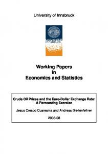
5.6. Impulse responses An alternative method for obtaining the information regarding the relationships among the variables is through the analysis of impulse response functions. The impulse response functions analyze the time profile of the effects of shocks on the future behavior of exchange rates and oil prices. Figs. 1 and 2 present the impulse response for oil price changes and exchange rate changes from one-standard deviation shock to exchange rates and oil prices. Series DLP and DLE are first difference of the natural logarithm of the crude oil prices and exchange rates, respectively. Fig. 1 shows the response of crude oil prices to exchange rate shock. The exchange rate shock has a significant negative impact on crude oil prices. The graph shows that the response of crude oil prices to shocks in exchange rates starts to decline in the second month, but increases after the third month.
6. Contributions, implications and conclusions This paper has empirically examined the dynamic behavior of the U.S. imported crude oil prices and exchange rates using the Granger causality test, and variance decomposition and impulse response function analysis. It was shown that exchange rates Granger-caused crude oil prices between the third month and the seventh month. From the eighth month to the twelfth month, crude oil prices Granger-caused the exchange rates. This is consistent with the findings of Uddin et al. (2013) and Chen and Chen (2007) and
Response of DLP to Cholesky One S.D. DLE Innovation .010
Table 5 Pairwise Granger causality tests. Hypothesis
.005
et does not Granger cause pt
pt does not Granger cause et
0.00228 (0.9619) 1.31481 (0.2691) 3.79263⁎⁎ (0.0102) 2.96345⁎⁎ (0.0191) 2.52320⁎⁎ (0.0281) 2.15874⁎⁎ (0.0451) 1.77508⁎ (0.0892) 1.62980 (0.1127) 1.45527 (0.1607) 1.34450 (0.2024) 1.25285 (0.2480) 1.28005 (0.2253)
0.17084 (0.6795) 0.03581 (0.9648) 0.07356 (0.9742) 0.56748 (0.6863) 1.44034 (0.2075) 0.98363 (0.4351) 1.16250 (0.3221) 1.91317⁎ (0.0552) 1.79994⁎ (0.0649) 1.63055⁎ (0.0937) 1.69497⁎ (0.0703) 1.63619⁎ (0.0771)
.000
Number of lags 1 month lag 2 month lags 3 month lags 4 month lags 5 month lags 6 month lags 7 month lags 8 month lags 9 month lags 10 month lags 11 month lags 12 month lags
Note: The p-values are given in parentheses. ⁎ Indicates statistical significance at 10%. ⁎⁎ Indicates statistical significance at 5%.
-.005 -.010 -.015 -.020 -.025 2
4
6
8
10
12
14
16
18
20
22
24
Fig. 1. Impulse responses — the shock analysis (exchange rate shock on crude oil prices).
412
T. Brahmasrene et al. / Energy Economics 44 (2014) 407–412
Response of DLE to Cholesky One S.D. DLP Innovation
the commodity price increases, and the only way the general equilibrium in the global economy will be restored is through exchange rate adjustment. The supply of oil (mainly from the OPEC countries), and, consequently the price of oil have been heavily influenced by global politics. More recently, the level and volatility of oil pieces have been attributed to speculation in the futures markets. So, future research could explore these implications to determine the channel of influence that establishes the relationship between exchange rate shock and oil price fluctuation. Alternative models could be used to investigate the impact of expansionary or contractionary monetary policies on exchange rates and crude oil prices. Multiple factors such as domestic versus foreign inflation rates, domestic versus foreign nominal or real interest rates, current account balance, etc., that affect exchange rates can be included. Given that this paper contributes to the current literature by carrying a specific case study of the U.S., future research may also be directed towards the investigation in other countries since individual countries behave differently.
.004 .003 .002 .001 .000 -.001 -.002 -.003 -.004 -.005 2
4
6
8
10
12
14
16
18
20
22
24
Fig. 2. Impulse responses — the shock analysis (crude oil price shock on exchange rates).
Bénassy-Quéré et al. (2007). They find that exchange rate change affects the oil price in the short run and the causality runs from oil price to the U.S. dollar in the long run. Thus, the research acknowledges the contribution to existing knowledge and theory. In variance decomposition analysis, oil prices are affected by exchange rate changes at a minimal level. However, in the medium run and the long run, oil price shocks have a significant impact on exchange rate changes. In the impulse responses, the exchange rate shock has a significantly negative impact on crude oil prices, while the impulse response of the exchange rate variable to a crude oil price shock is insignificant. How can investors and policy makers use this information? The major finding is that crude oil price movements always come after currency fluctuations in the short run, while currency fluctuations always follow crude oil price movements in the long run. This should capture the attention of investors, financial managers and hedgers. It is vital to use this knowledge to adjust their portfolio holdings since changes in currency value have some effect on crude oil prices in the short run. For the purpose of diversification, the investment portfolio should involve crude oil and the commodities such as traded goods which are affected by the currency fluctuation in the opposite direction. In light of these findings, a deeper understanding of the impulse response analysis reveals an intuitive impact of exchange rates on crude oil prices. As manifested in these findings, when the U.S. dollar depreciates, the U.S. crude oil imports become more expensive. Another implication relies on the analysis of variance decomposition and establishes that oil price shocks have a significant impact on exchange rate changes in the medium run and long run. This implies that when world oil prices are stabilized, currency fluctuation and uncertainty can be minimized. Furthermore, the key for governments and policy makers to adjust various economic stabilization schemes that are in place in various oil exporting countries for greater stability may lie in a multilateral agreement on principles and practices for exchange rates, accompanied by a framework for macroeconomic policy coordination among these countries. In effect, the predominant influence of financial markets in determining the conditions under which governments design their macroeconomic and development policies may be reduced. These findings also have important implications for monetary policies and strategic risk management to influence exchange rates or crude oil prices. It would appear that the role of the crude oil prices and exchange rates could be prominent. For example, if a commodity is priced in the U.S. dollar and due to demand and/or supply shocks,
References Aloui, R., Aïssa, M.S.B., Nguyen, D.K., 2013. Conditional dependence structure between oil prices and exchange rates: a copula-GARCH approach. J. Int. Money Financ. 32, 719–738. Apergis, N., Miller, S.M., 2009. Do structural oil-market shocks affect stock prices? Energy Econ. 31 (4), 569–575. Basher, S.A., Sadorsky, P., 2006. Oil price risk and emerging stock markets. Glob. Financ. J. 17, 224–251. Basher, S.A., Haug, A.A., Sadorsky, P., 2012. Oil prices, exchange rates and emerging stock markets. Energy Econ. 34 (1), 227–240. Bénassy-Quéré, A., Mignon, V., Penot, A., 2007. China and the relationship between the oil price and the dollar. Energy Policy 35 (11), 5795–5805. Chen, S.-S., Chen, H.-C., 2007. Oil prices and real exchange rates. Energy Econ. 29 (3), 390–404. Cong, R.G., Wei, Y.-M., Jiao, J.-L., Fan, Y., 2008. Relationships between oil price shocks and stock market: an empirical analysis from China. Energy Policy 36 (9), 3544–3553. Coudert, V., Mignon, V., Penot, A., 2007. Oil price and the dollar. Energy Stud. Rev. 15 (2) Article 3. Ding, L., Vo, M., 2012. Exchange rates and oil prices: a multivariate stochastic volatility analysis. Q. Rev. Econ. Finan. 52 (1), 15–37. Engle, R.F., Granger, C.W.J., 1987. Co-integration and error correction: representation, estimation, and testing. Econometrica 55, 251–276. Feinberg, R.M., 1989. The effects of foreign exchange movements on U.S. domestic prices. Rev. Econ. Stat. 71, 505–511. Granger, C.W.J., 1969. Investigating causal relations by econometric models and crossspectral methods. Econometrica 37 (3), 424–438. Goldberg, P., Knetter, M., 1997. Goods prices and exchange rates: what have we learned? J. Econ. Lit. 35, 1243–1272. Gross, D.M., Schmitt, N., 1996. Exchange rate pass-through and rivalry in Swiss automobile market. Welwirtschaftliches Archiv. 132, 278–303. Gross, D.M., Schmitt, N., 2000. Exchange rate pass-through and dynamic oligopoly: an empirical investigation. J. Int. Econ. 52, 89–112. Huang, A.Y., Tseng, Y.-H., 2010. Is crude oil price affected by the U.S. dollar exchange rate? Int. Res. J. Finance Econ. 58, 109–120. Im, K.S., Pesaran, M.H., Shin, Y., 2003. Testing for unit roots in heterogeneous panels. J. Econ. 115 (1), 53–74. Jones, C.M., Kaul, G., 1996. Oil and stock markets. J. Financ. 51 (2), 463–491. Tiwari, A.K., Dar, A.B., Bhanja, N., 2013. Oil price and exchange rates: a wavelet based analysis for India. Econ. Model. 31, 414–422. Levin, A.L., Linb, C.-F., Chu, C.-S.J., 2002. Unit root tests in panel data: asymptotic and finite-sample properties. J. Econ. 108 (1), 1–24. Lizardo, R.A., Mollick, A.V., 2010. Oil price fluctuations and U.S. dollar exchange rates. Energy Econ. 32 (2), 399–408. Narayan, P.K., Narayan, S., Prasad, A., 2008. Understanding the oil price-exchange rate nexus for the Fiji Islands. Energy Econ. 30 (5), 2686–2696. Reboredo, J.C., 2012. Modelling oil price and exchange rate co-movements. J. Policy Model 34 (3), 419–440. Reboredo, J.C., Rivera-Castro, M.A., 2013. A wavelet decomposition approach to crude oil price and exchange rate dependence. Econ. Model. 32, 42–57. Turhan, I., Hacihasanoglu, E., Soytas, U., 2012. Oil prices and emerging market exchange rates. Working Paper No: 12/01. Central Bank of the Republic of Turkey. Uddin, G.S., Tiwari, A.K., Arouri, M., Teulon, F., 2013. On the relationship between oil price and exchange rates: a wavelet analysis. Econ. Model. 35, 502–507. Vo, M., Ding, L., 2011. Exchange Rates and Oil Prices: A Multivariate Stochastic Volatility Analysis. Available at Social Science Research, Network (SSRN): http://ssrn.com/ abstract=1746318. Yousefi, A., Wirjanto, T.S., 2003. Exchange rate of the U.S. dollar and the J curve: the case of oil exporting countries. Energy Econ. 25 (6), 741–765. Yousefi, A., Wirjanto, T.S., 2004. The empirical role of the exchange rate on the crude-oil price formation. Energy Econ. 26 (5), 783–799. Yousefi, A., Wirjanto, T.S., 2005. A stylized exchange rate pass-through model of crude oil price formation. OPEC Rev. 29 (3), 177–197.