CS229 Project Report - Aircraft Collision Avoidance

CS229 Project Report - Aircraft Collision Avoidance Rahul A. Panicker, Nikhil Nigam, Dev Rajnarayan. 16 December 2005.

1

Introduction

Existing Air Traffic Control (ATC) procedures rely completely on human supervision and control. However, with the burgeoning traffic demands, it has become necessary to find options for automated (and possibly decentralized) traffic control. In particular, the problem of aircraft collision avoidance is of great interest. However, current approaches, [1] [2], are either computationally intensive, or limited to a two-aircraft scenario. We draw inspiration from the two-aircraft case and the trajectories generated by Gokhan et al and propose a relatively simple rule-based scheme for collision avoidance. We call this a traffic circle-based method for 2-D collision avoidance.1

2

Preliminary issues

2.1

Circle of Minimum Radius

We started with the idea of identifying a strategy for traffic circle formation. This involves deciding the radius and position of the traffic circle, and a policy that aircraft follow to join and leave the traffic circle to avoid collision2 . The natural choice for the radius was to choose the smallest possible value. With k aircraft in a traffic circle, and minimum separation between aircraft rmin , we get the smallest radius of the traffic circle to be : rmin (1) Rmin = 2 sin(π/k) where di is the distance traveled by ith aircraft. There are k points on the circle corresponding to k aircraft and are assigned in order (aircrafts in particular sectors are assigned points in the same sector). It is observed that the problem is convex in the coordinates of the center of circle.

2.2

Clustering to form Circles

There is still the bigger problem of deciding how the aircraft will join the circle without colliding. Moreover, forming traffic circles for aircraft with arbitrary initial positions was found to lead to many pathological, highly suboptimal trajectories. Therefore, a clustering algorithm was used to cluster aircraft 1 Aircraft 2 Current

involved in an impending collision form a traffic circle, along which they safely move and leave appropriately. FAA definition of a collision is a separation of less than 5 n.mi horizontal and 1000 ft. vertical.

1

Nigam, Panicker, Gorur

CS229

December 16, 2005

with similar headings together, with the idea that these aircraft will first form a line, and subsequently, these lines lead to the traffic circle. This idea eventually blossomed into the ‘ski lift’ approach described in the next section. The clustering algorithm used was k-means, and the features used were simply the nominal headings of the aircraft.

3

The ‘ski lifts’ approach

The basic idea of the traffic circle is the following. If the aircraft involved in a collision can form a safe circle that they traverse tangentially, they can then leave the circle at any time and continue on to their original destinations. However, for this to hold, it means that we cannot have a sector of more than 180 degrees handled by a single traffic circle. This is because further collisions will be caused as the aircraft leave the circle. Therefore, we impose the restriction that at any given altitude (the 2-D problem that we address), all aircraft have velocities in a particular 120-degree sector. Then, if aircraft get onto the traffic circle, they are assured to be safe as long as they leave the traffic circle in one of the other two sectors. this is similar to the safe trajectory generated for the two aircraft case in [2]. Moreover, to avoid large changes of direction when aircraft join the circle, we further stipulate that there are predetermined lines that lead into this traffic circle, and that there are preset moving points along these lines which are guaranteed to be safe on the circle also. We can think of this as being similar to chairs on a ski lift. As long as the aircraft ‘get on’ a chair without colliding with other aircraft, they are safe as long as they are on the ski lift. The problem can be been reduced to the following. Given an assignment of aircraft to a particular chair on a ski lift, generate a trajectory that has no collisions with other aircraft assigned to the same ski lift. This way, a potentially large problem involving many aircraft is reduced to a much smaller problem involving only those aircraft assigned a ski lift. At the moment, assignment of aircraft to specific chairs on the ski lifts was done heuristically. Then, reinforcement learning was implemented to learn a strategy for ‘capturing’ the ski lift in a collision-free manner.

3.1

Reinforcement learning

Our RL problem for each ski lift has a continuous state space x, whose components x1 , y1 , x2 , . . . , xn , yn denote cartesian coordinates of all aircraft assigned that lift, relative to their assigned chairs. Without loss of generality, the lift is assumed to be moving along the positive x direction with speed vT . Time was discretized, and over each time segment, all aircraft were assumed to move at fixed speed. They choose heading angles in steps of 10 degrees. While not on the lift, they have a velocity vA = 1.2 vT (in k order that they can catch up with a moving lift), and a heading θ ∈ { 18 π}, k = 0, . . . , 35. The velocity of the aircraft in the lift-fixed coordinate system is given by vrel = [(vA cos(θ) − vT ) vA sin(θ)]T

(2)

Finally, the approach is decentralized, in that the actions only refer to the headings of one aircraft. The following reward structure was used. 1. Reward of 1e3 for achieving the target. 2

Nigam, Panicker, Gorur

CS229

December 16, 2005

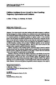
Figure 1: Value function for 4-D state space, shown for fixed opponent position 2. Penalty of -1e2 for leaving the vicinity of the assigned chair (rectangular region). 3. Penalty of -2e3 for colliding with another aircraft assigned to the same lift. 4. Reward of -10 for all other states. 5. Discount factor γ = 0.99. Value iteration was used to find the value function.

3.2

Value iteration: One or two aircraft

With only one or two aircraft, the state space is a compact subset of R2 or R4 , and the action space is a small number of discrete values. The value function is a function on a fairly small, albeit continuous space. Therefore, we resorted to gridding. However, to query the value function at any continuous state x, we used interpolation with the MATLAB function interpn. A version of Locally Weighted Linear Regression was also implemented in MATLAB , but in spite of using vectorized code, was much slower than the built-in interpolation. A plot of the value function for a one aircraft and one opponent is shown in figure (1).

3.3

Value iteration: Three aircraft case

With two or more opponents, the state space is now at least 6 dimensional. This proved too large for naive gridding. Therefore, we attempted to fit a polynomial to the value function, as shown in figure (2) Using a MATLAB toolbox soscode [3], we were able to generate polynomials of arbitrary degree in 6 dimensions. We generated polynomials of degree less than 7. Note that a degree 6 polynomial in 6 variables has upto 924 monomials. However, we found that although the value function passed through specified points (like 1e3 at the target), the process of value iteration based on this polynomial fit did not converge. Therefore, we used the following heuristic to compute an ‘approximate’ value function. For any position of a single opponent, we have the 4-dimensional value function from the interpolated grid

3

Nigam, Panicker, Gorur

CS229

December 16, 2005

Figure 2: Polynomial fit to value function, shown for fixed opponent positions described in the previous section. Now, given some configuration of two opponents, we approximated the value function by the average of the values corresponding to each of the single opponents separately. More precisely, V6D (x1 , y1 , x2 , y2 , x3 , y3 ) =

4

1 (V4D (x1 , y1 , x2 , y2 ) + V4D (x1 , y1 , x3 , y3 )) . 2

(3)

Simulation results

Shown overleaf are plots of the k-means clustering algorithm, and snapshots from the simulation of the decentralized optimal policy for 9 aircraft, split into three ski lifts of three aircraft each.

5

Future work

A major drawback of our approach is that dynamics of the aircraft were neglected. Still, the time and space scales of the collision-avoidance problem are so large that many details of the dynamics are truly negligible (for instance, one unit on the plots shown symbolizes the rather large distance of 5 nautical miles). The one aspect that is meaningful to include is the fact that though aircraft can be assumed to change turn rate instantaneously, they cannot be assumed to change heading instantaneously. This increases the dimension of our state space by one - for each time interval, the aircraft can choose a finite heading chage ∆θ in a certain allowable change. θ becomes a state variable that is not controlled explicitly. With increased memory, it should be possible to attack parametrized models like the polynomial model described earlier. However, it might be necessary to go to higher order polynomials.

4

Nigam, Panicker, Gorur

CS229

December 16, 2005

Figure 3: Simulation results

References [1] R. Ghosh and C. J. Tomlin, ”Maneuver design for multiple aircraft conflict resolution”, in Proc. American Control Conference, Chicago, IL, June 2000. [2] Tomlin, C. J. Mitchell, I. Ghosh, R., ”Safety Verification of Conflict Resolution Maneuvers”, IEEE Transactions on Intelligent Transportation Systems, 2001, Vol 2; Numb 2, pages 110-120 [3] http://www.stanford.edu/˜lall/soscode

5