[8] and probabilistic pushdown automata [5], as well as on transient analysis of .... that is, the so-called steady-state probability, for a single stable M|M|1 queue.
CSL model checking algorithms for infinite-state structured Markov chains
⋆
Anne Remke and Boudewijn R. Haverkort University of Twente Design and Analysis of Communication Systems Faculty for Electrical Engineering, Mathematics and Computer Science [anne,brh]@cs.utwente.nl
Abstract. Jackson queueing networks (JQNs) are a very general class of queueing networks that find their application in a variety of settings. The state space of the continuous-time Markov chain (CTMC) that underlies such a JQN, is highly structured, however, of infinite size in as many dimensions as there are queues. We present CSL model checking algorithms for labeled JQNs. To do so, we rely on well-known product-form results for the steady-state probabilities in (stable) JQNs. The transient probabilities are computed using an uniformization-based approach. We develop a new notion of property independence that allows us to define model checking algorithms for labeled JQNs.
1
Introduction
Queueing networks have been used for about half a century now, for modeling and analyzing a wide variety of phenomena in computer, communication and logistics systems. Seminal work on queueing networks was done by Jackson in the 1950s [11, 12]; in which he developed an important theorem that characterizes the steady-state (long-run) probabilities to reside in certain states in a restricted class of queueing networks (see the next section). However, there are many phenomena in the above classes of systems that cannot be studied well using these long-run probabilities. In communication system models, the following situations reflect such cases: (i) what is the probability that starting from an initial empty system, within t time-units, at least ki packets are buffered at queue i? (ii) what is the probability that starting from an overload situation, e.g., characterized by at least L packets at each queue, within t time-units, a low load situation, e.g., characterized by at most l 0 is allowed). A state in a JQN can be defined as s = (s1 , s2 , · · · , sn ), where si ≥ 0 represents the number of customers in queue i. A more precise discussion of the state space S is postponed to Section 3. For model checking purposes, we also need a state labeling. This leads us to the following definition. Definition 1 (Jackson queueing networks) A labeled Jackson queueing network LJQN J of order n (with n ∈ N+ ) is a tuple (λ, µ, R, L) with arrival rate λ, a vector of size n of service rates µ, a routing matrix R ∈ R(n+1)×(n+1) and a labeling function L that assigns a set of valid atomic propositions from a fixed and finite set AP of atomic propositions 2 to each state s = (s1 , s2 , . . . , sn ). Restriction 1 In the following we will restrict ourselves to atomic propositions of the form Vn < i=1 (si ≥ mi ) for mi ∈ N. This restricts the formulas we are able to check.
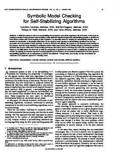
Example 1 In Figure 1(a) we present a LJQN with two queues that will serve as running example. The external arrival rate is λ, the rates is given as vector of service � � 0 r0,1 r0,2 µ1 and the routing matrix is R = r1,0 0 r1,2 . The labeling L will µ= µ2 r2,0 r2,1 0 be introduced later.
Definition 2 (Traffic equations) Pn The overall flow of jobs through each queue j is given as: λj = λr0,j + i=1 λi ri,j , for j = 1, . . . , n. These equations are called (first-order) traffic equations. 2 Definition 3 (Utilization) The utilization per queue i is defined as ρi =
λi µi .
2
Restriction 2 In case all ρi = λµii < 1, the QN is said to be stable. That is the number of arriving jobs per unit time is smaller than the amount of jobs that each queue can handle per unit time. This guarantees that the queue will not build up infinitely. In the following we restrict ourselves to stable LJQNs, to be able to compute steady-state probabilities.
The long-run probability that s customers are presently in a single M |M |1 queue, that is, the so-called steady-state probability, for a single stable M |M |1 queue (with ρ = µλ < 1) is: Pr{S = s} = (1 − ρ)ρs , where S is the random variable indicating the number of customers in the queue [13]. In [11, 12], Jackson proved the following theorem: Theorem 1 (Jackson) The overall steady-state probability distribution under restriction 2 (stability) is the product of the per-queue steady-state probability distributions, where the queues can be regarded as if operating independently from each other: Pr{S = s} =
n Y
(1 − ρi )ρsi i ,
s = (s1 , . . . , sn ) ∈ S.
(1)
λ1
λ1 µ2 · r2,0
2 1,
·r
µ1
µ2 · r2,0
µ1
µ2 · r2,0
2 1,
2 1,
·r
µ1 2 1,
µ2 · r2,0
·r λ1
.
λ2
·r
..
1 2,
µ1
.
λ2
·r
µ2 · r2,0
..
µ2
(a) two queues with feedback
1 2,
1 2,
λ1 µ · r1,0
...
µ · r1,0 λ2
·r
r2,0
·r
λ2
λ1
µ2
µ2
λ2
λ2
1 2,
λ1 µ · r1,0
r2,1
r0,2
·r
r1,2
λ0
...
µ · r1,0
µ2
µ2
r1,0 r0,1
λ2
µ1
µ2 · r2,0
µ · r1,0
λ1
...
.
.
...
..
..
...
i=1
...
µ · r1,0
(b) underlying state-space
Fig. 1. JQN with two queues
3
State space, transitions, independence and paths
This section addresses in detail the underlying state space of a LJQN. In Section 3.1 the underlying infinite state structured Markov chain is described. Section 3.2 explains how the infinite state space can be structured using atomic propositions and a new notion of independence is introduced. In Section 3.3 we define paths and transient as well as steady-state probabilities on LJQNs. 3.1
Infinite state structured Markov chain
The underlying state space of a LJQN J of order n is a highly structured labeled infinite-state continuous-time Markov chain with state space S = Nn that is infinite in n dimensions. Every state s ∈ S can be represented as an n-tuple s = (s1 , s2 , · · · , sn ), with si ≥ 0. The labeling function L : S → 2AP on the state space then assigns from the set AP of atomic propositions the set of valid atomic propositions to each state. The state sˆ = (0, . . . , 0) is called origin. As
the number of customers in queue i is restricted to si ≥ 0, for all i ∈ {1, . . . , n}, the underlying state-space is limited towards the origin in every dimension. An n dimensional state space S is bounded by n so-called boundary hyperplanes of dimension n − 1. Note that these boundary hyperplanes consist of an infinite number of states for n ≥ 2. State changes may occur due to an arrival at queue i from the environment or a departure to the environment from queue i, or by routing of a customer from queue i to queue j for 1 ≤ i, j ≤ n. By adding a state change vector to the source state, the destination state is defined: an arrival at queue i is denoted by the vector ai , a departure from queue i is denoted by the vector di , and a job routing from queue i to queue j is denoted as vector f i,j , with: ( ( fk = −1 k = i, ai =
aj = 1 aj = 0
i = j, j 6= i.
di =
dj = −1 dj = 0
j = i, j 6= i.
f i,j =
fk = 1 fk = 0
k = j, otherwise.
Note that an arrival is always possible, the new state is then defined as s′ = s+ai . A departure or a job routing from queue i is only possible, when there is at least one customer in queue i; in this case the new state s′ is computed as: s′ = s + di or s′ = s + f i,j , respectively. Definition 4 (Generator function) The rate for a state change from a state s to another state s′ within the infinite state space S is given by the generator function G(s, s′ ) : S × S → R+ , for s 6= s′ , as follows: cause restriction arrival none departure si > 0 routing si > 0
state change s′ = s + ai s′ = s + di s′ = s + f i,j
G(s, s′ ) λ · r0,i µi · ri,0 µi · ri,j
and G(s, s′ ) = 0 for s 6= s′ in all other cases. G(s, s) is defined as the negative sum over all possible outgoing rates from s, that is ! n X µi · 1si >0 , G(s, s) = − λ + i=1
where the indicator function 1si >0 returns 1 if si > 0, and 0 otherwise.
2
Example 2 Figure 1(b) shows the underlying state space of the LJQN from Example 1 that is infinite in two dimensions. Arrivals occur in both dimensions with rate λ · r0,1 and λ · r0,2 , departures happen from both dimensions with rates µ1 · r1,0 and µ2 · r2,0 , respectively, and jobs are routed from queue 1 to queue 2 with rate µ1 · r1,2 and from queue 2 to queue 1 with rate µ2 · r2,1 . 3.2
Independence of atomic propositions
Vn Recall that we restrict ourselves to atomic propositions of the form i=1 (si < ≥ mi ) for mi ∈ N. Due to this restriction, the validity of an atomic proposition does not
change anymore for si ≥ mi onwards for dimension i. Hence, we can define the so-called independence vector m = (m1 , . . . , mn ) and call the atomic proposition independent as of m. For the set of states {s ∈ S | ∀i(si ≥ mi )} the validity of the atomic proposition remains the same. The state space can be partitioned into a finite set of boundary states Sb and a finite number of infinite representative sets of states (denoted Sr ) such that the validity of an atomic proposition ap ∈ AP does not change any more in this set. We choose a representative state r for each of these infinite sets Sr such that for all s ∈ Sr the labeling does not change: L(r) = L(s), for all s ∈ Sr . In general, in an n-dimensional LJQN, there are n types of representative sets that account for 1 up to n infinite dimensions. A representative set is called infinite in dimension i if and only if ri = mi , and restricted in dimension i otherwise. In case a representative state r is infinite in k dimensions it represents a k dimensional set Sr , such that ( si ≥ ri iff ri = mi , s ∈ Sr ⇔ si = ri otherwise. Hence, a state s belongs to Sr when it takes the same value as r in the restricted dimensions and any value ≥ ri in the infinite dimensions. For atomic propositions, the origin sˆ represents the finite set of boundary states that is defined as Sb = {s ∈ S | si < mi , ∀i ∈ {1, . . . , n}}. The finite union of all representative states is called representative front and definedSas R(m) = {r ∈ S | ∃i : (ri = mi ) ∧ (∀j 6= i : (rj ≤ mj ))}. Note that S = Sb ∪ r∈R(m) Sr . For atomic propositions the representative front can be made smaller, however, for model checking CSL properties in general we need the full representative front as defined above. Example 3 Suppose we define the atomic proposition ap1 = (s1 ≥ 2)∧(s2 ≥ 3) for the LJQN from Example 1; the white states in Figure 2(a) then depict those states where ap1 is valid. The representative front for ap1 is formed by the states in the grey polygon: (0, 3) accounts for the states (0, j), with j ≥ 3, and (1, 3) represents the states (1, j) with j ≥ 3. For i ≥ 2, (2, 0) represents (i, 0), (2, 1) represents (i, 1) and (2, 2) represents (i, 2), respectively. These five representative states all account for a one dimensional set of states. The representative state (2, 3) accounts for the two-dimensional set of states S(2,3) = {s ∈ S | s1 > 2 ∧ s2 > 3}. The black states belong the the boundary set Sb with representative (0, 0). Example 4 Figure 2(b) shows the representative front for the atomic proposition ap2 = (s1 < 3) ∧ (s2 < 3) ∧ (s3 < 3) in a LJQN of dimension three. The atomic proposition is valid in the black states only (of the 27 only 9 are visible). All the remaining depicted states are representative states. We have different types of representative states: the white ones represent a set of states that is infinite in one dimension, the grey ones represent a set that is infinite in two dimensions and the light grey one (3, 3, 3) represents a set that is infinite in three dimensions.
queue 3
queue 2
representative state
e eu qu
2
representative set
queue 1 qu eu e
representative front
(a) 2-dim. state space
1
(b) 3-dim state space
Fig. 2. Representative front of states for independent atomic propositions
3.3
Paths and probabilities
In what follows, we first present the notion of path, before we define steady-state and transient state probabilities. Definition 5 (Paths) t0 t1 t2 . . . with, for i ∈ N, si ∈ S s1 −→ s2 −→ An infinite path σ is a sequence s0 −→ and ti ∈ R>0 such that G(si , si+1 ) > 0 for all i. A finite path σ of length t
t
tl−1
0 1 l + 1 is a sequence s0 −→ −− → sl such that sl is absorbing2 , and . . . sl−1 − s1 −→ G(si , si+1 ) > 0 for all i < l. For an infinite path σ, σ[i] = si denotes for i ∈ N the (i + 1)st state of path σ. The time spent in state si is denoted by δ(σ, i) = ti . Pi Moreover, with i the smallest index with t ≤ j=0 tj , let σ@t = σ[i] be the state occupied at time t. For finite paths σ with length l + 1, σ[i] and δ(σ, i) are defined in the way described above for i < l only and δ(σ, l) = σ[l] = ∞ and Pl−1 δ@t = sl for t > j=0 tj . P athJ (s) is the set of all finite and infinite paths in the LJQN J that start in state s and P athJ includes all (finite and infinite) paths of the LJQN J . 2
As for finite CTMCs, a probability measure on paths can now be defined depending on the starting state [3]. Starting from there, two different types of state probabilities can be distinguished. The transient state probability is a time-dependent measure that considers the LJQN at a given time instant t. The probability to be in state s′ at time instant t, given initial state s, is denoted as VJ (s, s′ , t) = Pr{σ ∈ P athJ (s) | σ@0 = s ∧ σ@t = s′ }. The transient probabilities are characterized by a linear system of differential equations of infinite size. Let V(t) be the matrix of transient state probabilities at time t for all possible starting states s and for all 2
A state s is called absorbing if for all s′ the rate G(s, s′ ) = 0.
possible goal states s′ (we omit the superscript J for brevity here), then we have V′(t) = V(t) · G, given V(0) = I. An efficient method to compute the transient probabilities will be discussed in Section 5.4. The steady-state probabilities to be in state s′ , given initial state s, are defined as π J (s, s′ ) = limt→∞ VJ (s, s′ , t), and indicate the probabilities to be in some state s′ “in the long run”. If steady-state is reached, the above mentioned derivatives V′(t) will approach zero. As we require stable queues the underlying state space of the LJQN is ergodic and, the initial state does not influence the steady-state probabilities (we therefore write π(s′ ) instead of π(s, s′ ) for brevity). In the context of LJQNs the steady-state probabilities per state can be computed using the product-form of Theorem 1.
4
The logic CSL
We use the logic CSL [3] to express properties for LJQNs. The syntax and semantics are the same as for finite CTMCs, with the only difference that we now interpret the formulas over states and paths in LJQNs. Let p ∈ [0, 1] be a real number, ⊲⊳ ∈ {≤, , ≥} a comparison operator, t1 , t2 ∈ R+ real numbers and AP a set of atomic propositions with ap ∈ AP . CSL state formulas Φ are defined by Φ ::= tt | ap | ¬Φ | Φ ∧ Φ | S⊲⊳p (Φ) | P⊲⊳p (φ), where φ is a path formula constructed by φ ::= X [t1 ,t2 ] Φ | Φ U [t1 ,t2 ] Ψ. For a CSL state formula Φ and a LJQN J , the satisfaction set Sat(Φ) contains all states of J that fulfill Φ and is computed with a recursive descent procedure over the parse tree of Φ, as for CTL [7]. Satisfaction is stated in terms of a satisfaction relation |=. The relation |= for states and CSL state formulas is defined as: s |= tt for all s ∈ S, s |= ap iff ap ∈ L(s), s |= ¬Φ iff s 6|= Φ,
s |= Φ ∧ Ψ iff s |= Φ and s |= Ψ, s |= S⊲⊳p (Φ) iff π J (s, Sat(Φ)) ⊲⊳ p, s |= P⊲⊳p (φ) iff P robJ (s, φ) ⊲⊳ p,
P where π J (s, Sat(Φ)) = s′ ∈Sat(Φ) π J (s, s′ ), and P robJ (s, φ) describes the probability measure of all paths σ ∈ P ath(s) that satisfy φ when starting in state s, that is, P robJ (s, φ) = Pr{σ ∈ P athJ (s) | σ |= φ}. The steady-state operator S⊲⊳p (Φ) denotes that the steady-state probability for Φ-states meets the bound p. P⊲⊳p (φ) asserts that the probability measure of the paths satisfying φ meets the bound p. The next operator X [t1 ,t2 ] Φ states that a transition to a Φ-state is made between t1 and t2 . The until operator Φ U [t1 ,t2 ] Ψ asserts that Ψ is satisfied
at some time instant in between [t1 , t2 ] and that at all preceding time instants Φ holds. The relation |= for paths and CSL path formulas is defined as: σ |= X [t1 ,t2 ] Φ σ |= Φ U
[t1 ,t2 ]
iff σ[1] is defined and σ[1] |= Φ and t1 ≤ δ(σ, 0) ≤ t2 , Ψ
iff ∃t(t1 ≤ t ≤ t2 ) (σ@t |= Ψ ∧ (∀t′ ∈ [0, t)(σ@t′ |= Φ))).
From [15] we know that CSL formulas are not level independent on QBDs in general, even if the atomic propositions are level independent. However, their validity does not change arbitrarily between levels. In the following we will show that for CSL formulas on LJQNs we can also find a state from which the validity of the CSL formula does not change anymore. Definition 6 (Independence of CSL formulas) Let J be a LJQN of order n. A CSL state formula Φ is independent as of m if and only if there exists a finite representative front R(m) = {r ∈ S | ∃i(ri = mi ) ∧ (∀j 6= i(rj ≤ mj ))} such that for all r ∈ R(m) and for all s ∈ Sr it holds 2 that r |= Φ ⇔ s |= Φ. The following propositions states, under the assumption of independent atomic propositions as of m, that such a finite representative front R(m′ ) exists for any CSL state formula. We will justify this proposition inductively over the structure of the logic in Section 5. Proposition 1 Let J be a LJQN of order n with independent atomic propositions as of m and let Φ be a CSL state formula other than P⊲⊳p (Φ U [t1 ,t2 ] Ψ ). Then there exists a finite representative front R(m′ ) such that the validity of Φ does not change within each subset Sr for r ∈ R(m′ ) in J . For the until operator P⊲⊳p (Φ U I Ψ ) we assume that for no state s the probability measure is exactly equal to p. Under this assumption, there exists a vector m′ , such that P⊲⊳p (Φ U I Ψ ) is independent as of m′ in J . 2 For a CSL formula that is independent as of m, the satisfaction set can be considered as the union of the boundary satisfaction set SatSb (Φ) = Sb ∩ Sat(Φ) and the representative satisfaction front SatR(m) (Φ) = R(m) ∩ Sat(Φ). The representative state r ∈ R(m) then represent the remaining infinite state space.
5
Model checking algorithms
In this section we present model checking algorithms for CSL. In Section 5.1 we explain how independence changes when applying logical operators. We explain how to model check the steady-state operator in Section 5.2, the next operator in 5.3 and the until operator in Section 5.4, including a discussion on how to compute transient probabilities in LJQNs.
5.1
Logical operators
The model checking procedure for logical operators is the same as for finite CTMCs. The only thing we need to take care of is how independence changes. Negating a CSL formula does not change its independence. For a CSL formula Φ that is independent as of m the negation ¬Φ is also independent as of m. However, combining a CSL formula Φ that is independent as of mΦ with a CSL formula Ψ that is independent as of mΨ with conjunction, changes independence depending on the structure of Φ and Ψ . In any case, we can state that Φ ∧ Ψ is independent as of m = max{mΦ , mΨ }, where we choose the maximum of mΦ i and mΨ i in every dimension i. Note that this new independence vector m might be too pessimistic, depending on the structure of Φ and Ψ . 5.2
Steady-state operator
Theorem 1 states the steady-state probabilities in a JQN. A state s satisfies S⊲⊳p (Φ) if the sum of the steady-state probabilities of all Φ-states reachable from s meets the bound p. Since a JQN is by definition ergodic, the steady-state probabilities are independent of the starting state. It follows that either all states satisfy a steady-state formula or none of the states does, which implies that a steady-state formula is always independent as of m = (0, . . . , 0). We sum the steady state probabilities of all states that satisfy Φ by summing over all states s ∈ Sr for r |= Φ and over all states from Sb that satisfy Φ: X X X p(s) ⊲⊳ p p(s) + s |= S⊲⊳p (Φ) ⇔ (2) s∈Sb , s∈Sat(Φ)
r∈R(m), r∈Sat(Φ)
s∈Sr
We obtain Sat(S⊲⊳p (Φ)) = S, if the accumulated steady-state probability meets the bound p otherwise Sat(S⊲⊳p (Φ)) = ∅. In case the representative state r ∈ Sat(Φ), all states s ∈ Sr are in Sat(Φ). The accumulated steady-state probability for all states s ∈ Sr is given by the following expression: ( n Y X (1 − ρi )ρri i for ri 6= mi , p(s) = Ω(i), with Ω(i) = (3) i for ri = mi . ρm i i=1 s∈S r
In this expression we distinguish between the finite and the infinite dimensions of a representative state r. In a finite dimension i we multiply with (1 − ρi )ρri i i and in an infinite dimension i we multiply with ρm i . Proof 1 (Accumulated steady-state probability) Applying Jackson’s Theorem, the accumulated steady-state probability is given by ! n X Y X si (4) (1 − ρi )ρi . p(s) = s∈Sr
Recall that
s ∈ Sr ⇔
s∈Sr
(
i=1
si ≥ ri si = ri
iff ri = mi , otherwise.
According to Jackson’s Theorem we can consider the dimensions independently from each other. Hence, for every dimension i = 1, . . . , n, a state s ∈ Sr may take all values j ≥ mi in case ri = mi and the value ri in case ri 6= mi . Thus, ( n Y X for ri 6= mi , (1 − ρi )ρri i p(s) = Ω(i), with Ω(i) = P∞ (5) j for ri = mi . j=mi (1 − ρi )ρi i=1 s∈S r
The infinite sum can be rewritten ∞ X
(1 −
ρi )ρji
= (1 − ρi )
∞ X
ρji = (1 − ρi )
j=mi
j=mi
i ρm i i = ρm i 1 − ρi
and replaced to match (3): Ω(i) =
(
(1 − ρi )ρri i i ρm i
for ri 6= mi , for ri = mi . 2
Example 5 We want to check the CSL formula S⊲⊳p ((s1 ≥ 2) ∧ (s2 ≥ 3)). Recall from Example 3 that all states r ∈ R((2, 3)) = {(0, 3), (1, 3), (2, 0), (2, 1), (2, 3)} satisfy ap1 = (s1 ≥ 2) ∧ (s2 ≥ 3) and the boundary states do not satisfy ap1 . Using (2) and (3) and accumulating the probabilities for all representative states r ∈ R((2, 3)) we obtain s |= S⊲⊳p ((s1 ≥ 2) ∧ (s2 ≥ 3)) ⇔
5.3
� (1 − ρ1 )ρ32 + (1 − ρ1 )ρ1 ρ32 + ρ21 (1 − ρ2 ) + ρ21 (1 − ρ2 )ρ2 + ρ21 ρ32 ⊲⊳ p.
(6)
Time-bounded next operator
The time-bounded next operator for LJQNs is computed just as for QBDs [15]. Recall that a state s satisfies P⊲⊳p (X [t1 ,t2 ] Φ) if the one-step probability to reach a state that fulfills Φ within a time t ∈ [t1 , t2 ], outgoing from s meets the bound p. The possibly infinite summation over all Φ-states can be truncated by only considering those Φ-states that can be reached in one step from s. We define the set of states that is reachable in one step from state s as Bs = {s′ ∈ S|G(s, s′ ) > 0}. Note that Bs is always finite. We then have: s |= P⊲⊳p (X [t1 ,t2 ] Φ) ⇔ Pr{σ ∈ P ath(s) | σ |= X [t1 ,t2 ] Φ} ⊲⊳ p � � ′ X G(s, s ) ⇔ eG(s,s)·t1 − eG(s,s)·t2 · ⊲⊳ p, −G(s, s) s′ ∈Sat(Φ)∩B s6=s′
(7)
s
where eG(s,s)·t1 − eG(s,s)·t2 is the probability of residing in s for a time t ∈ [t1 , t2 ], G(s,s′ ) and −G(s,s) specifies the probability to step from state s to state s′ , provided a step takes place.
Now, let the inner formula Φ be independent as of m. Hence, the validity of Φ might be different for all states s ∈ Sb . Therefore, the representative states r ∈ R(m) may satisfy P⊲⊳p (X [t1 ,t2 ] Φ), whereas the remaining states s ∈ Sr do not necessarily satisfy P⊲⊳p (X [t1 ,t2 ] Φ), since Sb is reachable in one step. However, from m + 1 (with 1 = (1, 1, . . . , 1, 1)) onwards, with one step only states with equivalent Φ validity can be reached. Thus, in case the inner formula Φ is independent as of m, P⊲⊳p (X [t1 ,t2 ] Φ) is independent as of m + 1. For the construction of the satisfaction set of such a formula we have to compute explicitly the satisfying states in Sb . SatR(m+1) (P⊲⊳p (X [t1 ,t2 ] Φ)) then provides the validity of P⊲⊳p (X [t1 ,t2 ] Φ) for the remaining infinite state space S \ Sb . 5.4
Until operator for I = [0, t]
For model checking P⊲⊳p (Φ U I Ψ ) we adopt the general approach for finite CTMCs [3] and QBDs [15]. Recall that the CSL path formula ϕ = Φ U I Ψ is valid if a Ψ -state is reached on a path during the time interval [t1 , t2 ] via only Φ-states. We restrict ourselves to intervals of the form I = [0, t]. The future behavior of the LJQN is then irrelevant for the validity of ϕ, as soon as a Ψ -state is reached. Thus all Ψ -states can be made absorbing without affecting the satisfaction set of formula ϕ. On the other hand, as soon as a (¬Φ ∧ ¬Ψ )-state is reached, ϕ will be invalid, regardless of the future evolution. As a result of the above consideration, we may switch from checking the LJQN J to checking a new, derived, LJQN, denoted as J [Ψ ][¬Φ∧¬Ψ ] = J [¬Φ∨ Ψ ], where all states in the underlying Markov chain that satisfy the formula in ˜ s′ ) for J [¬Φ ∨ square brackets are made absorbing. The generator function G(s, Ψ ] is then defined as ( G(s, s′ ), s 2 ¬Φ ∨ Ψ, ′ ˜ (8) G(s, s ) = 0, otherwise, ˜ s) is adapted accordingly. Model checking a formula involvfor s 6= s′ . G(s, ing the until operator then reduces to calculating the transient probabilities π J [¬Φ∨Ψ ](s, s′ , t) for all Ψ -states s′ . Exploiting the structure of LJQNs yields s |= P⊲⊳p (Φ U [0,t] Ψ ) ⇔ Prob J (s, Φ U [0,t] Ψ ) ⊲⊳ p ∞ X X X π J [¬Φ∨Ψ ](s, s′ , t) + ⇔ s′ ∈SatSb (Ψ )
i=0 s′ ∈SatR(m+i) (Ψ )
π J [¬Φ∨Ψ ](s, s′ , t) ⊲⊳ p.
(9)
The transient probabilities are accumulated for the Ψ states in Sb and for the Ψ states in the representative front R(m + i) for i ∈ N. Note that these representative fronts are situated in layers around Sb and cover the infinite state space S \ Sb for i ∈ N. In [15] we have shown how transient probabilities can be computed for QBDs using uniformization [9] by considering only a finite fraction of the infinite state
space. As standard property of uniformization, the finite time bound t is transformed to a finite number of steps l [9]. To do the same for LJQNs, first the ˜ for the embedded DTMC is defined as probability function P(s, s′ ) (or for P) ′ G(s,s ) P(s, s′ ) = for s 6= s′ and P(s, s) = G(s,s) + 1. The uniformization conν ν stant ν must be at least equal to the maximum of the negative rates G(s, s); for P LJQNs, the value ν = λ + ni=1 µi suffices. For an allowed maximal numerical error ε, uniformization requires a finite number l of steps (state changes) to be taken into account in order to compute the transient probabilities; l can be computed a priori, given ε, ν and t. Summarizing, we have obtained the following result: If ¬Φ ∨ Ψ is independent as of m then using uniformization with l steps, we obtain the same transient probabilities for states s ∈ Sr , with r ∈ R(m+l), since from all states s ∈ Sr , only corresponding states can be reached when taking l steps in the LJQN.
queue 2
m+l
m
Example 6 The figure to the left shows the finite fraction of the infinite state space that is needed to compute the validity of P⊲⊳p (Φ U I Ψ ). Starting from every representative state r ∈ R(m + l), still l steps can be undertaken in every direction without reaching the boundary set Sb . The total amount of states we have to consider equals (m1 + l) · (m2 + l), from which m1 + m2 + 2l − 1 are representative states.
queue 1
For all states s ∈ S, we add the computed transient probabilities to reach any Ψ -state and check whether the accumulated probability meets the bound p. We define the accumulated probability for up to l steps in the uniformized Markov chain as: π ˜ (l) =
X
s′ ∈SatSb (Ψ )
π J [¬Φ∨Ψ ](s, s′ , t) +
l−1 X
X
π J [¬Φ∨Ψ ](s, s′ , t) (10)
i=0 s′ ∈SatR(m+i) (Ψ )
Note that the above expression, for l → ∞, equals the exact probability that is to be compared with p in (9). Once the accumulated probabilities are calculated, similar inequalities as presented in [15], can be used to decide the validity of P⊲⊳p (Φ U I Ψ ) on LJQNs. The accumulated probability is always an underestimation of the actual probability. The value of the maximum error ε accumulated for all states and depending on the number of steps l decreases as l increases. Thus, we obtain the following implications: (a) π ˜ (l) (s, Sat(Ψ ), t) > p ⇒ π(s, Sat(Ψ ), t) > p (l) (b) π ˜ (s, Sat(Ψ ), t) < p − ε ⇒ π(s, Sat(Ψ ), t) < p
If one of these inequalities (a) or (b) holds, we can decide that the bound < p or > p is met. For the bounds ≤ p and ≥ p, similar implications can be given. If π ˜ (s, Sat(Ψ ), t) ∈ [p, p − ε], we cannot decide whether π(s, Sat(Ψ ), t) meets the bound p. In this case, increasing l resolves the problem. However, note that in case p = π(s, Sat(ψ), t) we cannot decide and iteration does not stop. As already mentioned, for all representative states r ∈ R(m + l) the transient probabilities for all s ∈ Sr computed with l steps will be the same. Thus, if we can decide whether the bound p is met (case (a) or (b) above), we can be sure that P⊲⊳p (Φ U [0,t] Ψ ) is independent as of m+l. In that case, we check for all states s ≤ m + l whether the accumulated transient probability of reaching a Ψ -state meets the bound p. The states s ∈ Sb that satisfy P⊲⊳p (Φ U [0,t] Ψ ) form the boundary satisfaction set SatSb and the representative states that satisfy P⊲⊳p (Φ U [0,t] Ψ ) form the representative satisfaction set SatR(m+l) (P⊲⊳p (Φ U [0,t] Ψ )). Qn For model checking the until operator we need to consider i=1 (mi + 2l) states in total, depending on the number of steps l considered, the dimension n of the LJQN, Q and the independence vector m of the inner formula. Hence, Q n n (m + 1) − i i=1 mi representative states suffice to represent the infinite i=1 states space S \ Sb . In [16] we presented a method to efficiently compute the transient probabilities in QBDs and check the until operator with a so-called dynamic stopping criterion. This method can also be applied to LJQNs. When iteratively computing the approximation π ˜ (l) (s, Sat(Ψ ), t) and regularly checking whether either (a) or (b) holds for all starting states, the number of considered steps with uniformization is minimized. It is expected that such an approach will lead to similar efficiency improvements.
6
Conclusions
In this paper we presented model checking algorithms for checking CSL properties for a very general class of queueing networks, namely for labeled Jackson queueing networks. The underlying state space of such LJQNs is a highly structured CTMC that is, of infinite size in as many dimensions as there are queues. We introduce a new notion of property independence on LJQNs that is needed for model checking. Steady-state probabilities are computed in (stable) LJQNs with well-known product-form results and transient probabilities are computed with an adaption of our uniformization-based approach. We provided a running example throughout the paper to illustrate our approach. Note that the model checking procedure for LJQN as introduced in this paper, and the model checking procedure for QBDs [15], in their simplest setting, i.e., the case that the model is a simple M|M|1 queue (which is both a QBD and a LJQN), are in essence the same. At various points, the presented algorithms can be made more efficient. For instance, applying a dynamic stopping criterion (as in [16]) when model checking the until operator in LJQNs might considerably decrease the number of states
that has to be taken into account. To do so, we need to develop efficient data structures to store the step-wise computed probabilities. The complexity for checking the steady-state operator is linear in the number of queues and the complexity for checking the until operator is given by matrix vector multiplications of matrices that are exponential in the number of queues. V We restricted ourselves to atomic propositions of the form ni=1 (si < ≥ mi ) for mi ∈ N; this facilitates the determination of the independence vector m. For model checking other properties like the balance of queues or a general threshold, the notion of property independence needs to be (and can be) generalized. Finally, we developed the model checking algorithm for the until operator with time-bound in [0, t], however, other time intervals can be handled similarly as for finite state CTMCs or QBDs [3, 17]. In further work, we will introduce rewards to allow for CSRL model checking. Furthermore, we also consider addressing networks of QBDs. However, to the best of our knowledge, there is no method available to compute steady-state probabilities on such multi-dimensional QBDs, hence, we will have to do without the steady-state operator.
References 1. P. Abdulla, B. Jonsson, M. Nilsson, and M. Saksena. A survey of regular model checking. In Proc. 15th Int. Conference on Concurrency Theory (Concur’04), number 3170 in LNCS, pages 35–48, 2004. 2. A. Aziz, K. Sanwal, and R. Brayton. Model checking continuous-time Markov chains. ACM Transactions on Computational Logic, 1(1):162–170, 2000. 3. C. Baier, B.R. Haverkort, H. Hermanns, and J.-P. Katoen. Model-checking algorithms for continuous-time Markov chains. IEEE Transactions on Software Engineering, 29(7):524–541, 2003. 4. P. Ballarini and J. Hillston. Compositional csl model checking for boucherie product processes. In 3rd Workshop on Automated Verfication of Critical Systems (AVOCS’03), DSSE Technical Report DSSE-TR-2003-2, 2003. 5. T. Br´ azdil, A. Kucera, and O. Strazovsk´ y. On the decidability of temporal properties of probabilistic pushdown automata. In Proc. 22nd Annual Symposium on Theoretical Aspects of Computer Science (STACS’05), number 3404 in LNCS, pages 145–157. Springer, 2005. 6. G. Ciardo. Discrete-time Markovian stochastic Petri nets. In Computations with Markov Chains, pages 339–358. Raleigh, 1995. 7. E. Clarke, E. Emerson, and A. Sistla. Automatic verification of finite-state concurrent systems using temporal logic specifications. ACM Transactions on Programming Languages and Systems, 8(2):244–263, 1986. 8. K. Etessami and M. Yannakakis. Recursive Markov chains, stochastic grammars, and monotone systems of nonlinear equations. In Proc. 22nd Annual Symposium on Theoretical Aspects of Computer Science (STACS’05), number 3404 in LNCS, pages 340–352. Springer, 2005. 9. D. Gross and D.R. Miller. The randomization technique as a modeling tool and solution procedure for transient Markov processes. Operations Research, 32(2):343– 361, 1984. 10. P.G. Harrison. Transient behaviour of queueing networks. Journal of Applied Probability, 18(2):482–490, 1981.
11. J.R. Jackson. Networks of waiting lines. Operations Research, 5(4):518–521, 1957. 12. J.R. Jackson. Jobshop-like queueing systems. Management Science, 10(1):131–142, 1963. 13. L. Kleinrock. Queueing Systems; Volume 1: Theory. John Wiley & Sons, 1975. 14. T.I. Matis and R.M. Feldman. Transient analysis of state-dependent queueing networks via cumulant functions. Journal of Applied Probability, 38(4):841–859, 2001. 15. A. Remke, B.R. Haverkort, and L. Cloth. Model checking infinite-state markov chains. In Proc. 11th International Conference on Tools and Algorithms for the Construction and Analysis of Systems (TACAS’05), number 3440 in LNCS, pages 237–252. Springer, 2005. 16. A. Remke, B.R. Haverkort, and L. Cloth. Uniformization with representatives. In Proc. Workshop on Tools for solving structured Markov chains. ACM press (CD only), 2006. 17. A. Remke, B.R. Haverkort, and L. Cloth. CSL model checking algorithms for QBDs. Theoretical Computer Science, doi: 10.1016/j.tcs.2007.05.007, 2007. 18. Ph. Schnoebelen. The verification of probabilistic lossy channel systems. In Validation of Stochastic Systems, volume 2925 of LNCS, pages 445–465, 2004. 19. A.P.A. van Moorsel. Performability Evaluation Concepts and Techniques. PhD thesis, Dept. of Computer Science, University Twente, 1993.