CubeLSI: An Effective and Efficient Method for Searching ... - HKU CS

HKU CS Tech Report TR-2010-10

CubeLSI: An Effective and Efficient Method for Searching Resources in Social Tagging Systems Bin Bi, Sau Dan Lee, Ben Kao, Reynold Cheng {bbi, sdlee, kao, ckcheng}@cs.hku.hk Technical Report TR-2010-10 Department of Computer Science The University of Hong Kong 2010-11-16 Abstract In a social tagging system, resources (such as photos, video and web pages) are associated with tags. These tags allow the resources to be effectively searched through tag-based keyword matching using traditional IR techniques. We note that in many such systems, tags of a resource are often assigned by a diverse audience of causal users (taggers). This leads to two issues that gravely affect the effectiveness of resource retrieval: (1) Noise: tags are picked from an uncontrolled vocabulary and are assigned by untrained taggers. The tags are thus noisy features in resource retrieval. (2) A multitude of aspects: different taggers focus on different aspects of a resource. Representing a resource using a flattened bag of tags ignores this important diversity of taggers. To improve the effectiveness of resource retrieval in social tagging systems, we propose CubeLSI — a technique that extends traditional LSI to include taggers as another dimension of feature space of resources. We compare CubeLSI against a number of other tag-based retrieval models and show that CubeLSI significantly outperforms the other models in terms of retrieval accuracy. We also prove two interesting theorems that allow CubeLSI to be very efficiently computed despite the much enlarged feature space it employs.

1

Introduction

We are witnessing an increasing number of social tagging systems on the web, such as Flickr, Delicious, Bibsonomy, Last.fm and YouTube. These systems provide platforms on which various resources, such as photos, music, video and web sites, are shared. One of the distinctive characteristics of these social tagging systems is that resources are tagged by communities of users. Through manually-assigned tags, users can express their distinct interests on the various aspects of the resources. For example, a photo could be tagged with words that describe the subjects, people and places in the photo; the artistic elements of the photo; or the historical background of the photo. Given the collective wisdom of a user community, tagging amasses a tremendous amount of meta-data, which facilitates the organization and retrieval of resources. As an example, a project called “The Commons”1 was launched by Flickr in 2008 in which photography collections obtained from museums and libraries are displayed. One of the objectives of “The Commons” is to provide a way for the general public to contribute information and knowledge about the photos by means of written comments and tags. With their increasing popularity, social tagging systems have been growing at very high rates, both in terms of their user communities and resource collections. For example, Flickr had more than 32 million users as of May 20092 and hosted over 4 billion photos as of October 20093 . Last.fm had 30 million users and 1

http://www.flickr.com/commons

2 http://www.flickr.com/help/forum/en-us/97258/ 3 http://blog.flickr.net/en/2009/10/12/4000000000/

1

1

INTRODUCTION

more than 7 million tracks cataloged as of March 20094 . The sheer amount of resources made available by these systems calls for highly effective and scalable searching methods. Our goal is to study the properties of social tagging systems and to propose a novel tag-based technique to search for relevant resources. Our search technique, called CubeLSI, follows a typical keyword-based query model employed by major social tagging systems. In these systems, a user query is expressed by a few keywords (tags) and a ranked list of relevant resources is returned as the query result. A simple approach to this searching problem is to match the query keywords against the tags associated with each resource in a way that is similar to traditional document retrieval techniques. This approach, however, suffers from two complications that are intrinsic to social tagging systems. Firstly, taggers are typically untrained casual users who are free to pick their own tags. The tags thus come from an uncontrolled vocabulary rather than from a well-defined taxonomy. This results in ambiguities: a single tag could refer to multiple different concepts (polysemy) and a single concept could be described by different tags (synonymy). These make tags a noisy feature of resources in the retrieval process. Secondly, while a traditional document is usually written by a single author, a resource is typically tagged by a diverse audience of taggers. Different interest groups of taggers may focus on different aspects of the same resource. For example, a group of taggers may be interested in the photo-taking techniques (e.g., composition, color-tone, exposure, etc.) of a photo, while another group may be interested in its content (e.g., faces and places). An interesting implication to this observation is that not only “which tags are assigned to a resource” is important information, but also “who has assigned the tags,” which provides contexts to the tags, is important as well. For example, the tag “Apple” given by someone who is interested in digital image processing is likely referring to a computer on which a photo is digitally processed instead of referring to a fruit displayed in the photo. In this paper we propose CubeLSI, a tag-based resource retrieval technique that addresses the two problems, namely, tag-ambiguity and a multitude of aspects, as mentioned above. In a nutshell, CubeLSI applies Latent Semantic Indexing (LSI) [9, 10] to capture high-level semantic information of tags to improve the precision of resource retrieval. However, unlike traditional LSI, CubeLSI takes into account the tag-tagger relationship (i.e., which tags are assigned by whom) in performing semantic analysis. As we will see, our approach of taking taggers as a feature dimension significantly improves the quality of the semantic analysis. This results in more accurate resource retrieval. In the following, we further discuss how CubeLSI approaches the two problems. We will also give the general framework of CubeLSI. Tags, Concepts and Aspects As we have discussed, there are generally a multitude of aspects for a given resource. When a tagger tags a resource, he first studies the resource to identify certain aspects of his interest. For example, a tagger may be interested in the type of event (e.g., wedding) behind a picture of a bouquet instead of the kind of flower (e.g., roses) shown. The tagger then discovers the semantic concepts exhibited by the resource with respect to each chosen aspect, and expresses these concepts via a set of words (tags). Each concept thus corresponds to a semantically coherent group of tags. In our bouquet photo example, we have “type-of-event” being an aspect, “wedding/engagement/marriage” being a concept, and the word, say, “wedding” being a tag to express the concept. Similarly, when issuing a query, a user first comes up with the semantic concepts he is interested in, and then formulates his query by providing a few tags (e.g., marriage). To avoid the tag-ambiguity problem, the matching between queries and resources should be carried out at the semantic concept level. This makes it possible to match a given query with its relevant resources even if the query and the resources are described by disjoint sets of tags. Therefore, our CubeLSI approach transforms the bag of tags associated with a resource to a bag of concepts to enhance search quality. We call the process of extracting concepts from resources Concept Distillation. Resources, Taggers and Tags LSI is a popular semantic analysis technique that attempts to overcome the word ambiguity problem by extracting concepts from words in an unstructured text collection. Since LSI has proven to be remarkably successful in IR, our CubeLSI approach 4 http://blog.last.fm/2009/03/24/lastfm-radio-announcement

HKUCS TR-2010-10

2

1

INTRODUCTION

Table 1: Tag pairs and their semantic relations Human- CubeLSI LSI Tag Pairs judged hcomedy, humouri hvirus, antivirusi Y Y N hwireless, WiFii hcancer, charitiesi hshopping, photographyi N N Y hfestival, musici

adapts LSI to extract concepts from tag-based data. In traditional document retrieval systems, LSI performs Singular Value Decomposition (SVD) on a term-document matrix. (For a socialtagging system, this matrix corresponds to the tag-resource relation, i.e., which tags are assigned to which resource.) To extract concepts, LSI identifies terms (tags) that are highly semantically related. Essentially, two terms (tags) are related or similar if and only if they have very similar contexts, e.g., they occur in similar sets of documents (resources). As we have argued, besides the set of resources, taggers also represent a very important dimension of the tags’ feature space in social tagging systems. Therefore, CubeLSI extends LSI by considering the tagger dimension. More specifically, instead of applying SVD on a 2D tag-resource matrix, CubeLSI performs Tucker Decomposition on a third-order tensor whose dimensions are resources, taggers, and tags in order to discover semantically related tags. To further substantiate our claim that the tagger dimension improves tag semantic analysis, we give a preview of some of the empirical observations we made in our experiments. We conducted user studies on the Delicious dataset (see Section 6) to compare traditional LSI against CubeLSI in identifying the semantic relations of tags. Our general observation is that the semantic relations obtained by CubeLSI better resemble those identified by human observers. To illustrate, Table 1 shows a few tag pairs together with the results of their semantic relations derived from different schemes. A ‘Y’ denotes that two tags are highly semantically related, while an ‘N’ denotes that two tags are weakly semantically related. We see that the results under CubeLSI are consistent with those given by humans, whereas the results under LSI are not. These examples show the importance of the tagger dimension (which is used in CubeLSI) in measuring tag similarity. The CubeLSI Framework Figure 1 shows the CubeLSI framework for tag-based searching of resources in social tagging systems. The framework consists of an offline concept-extraction component and an online query-processing component. For the offline component, tag assignments are represented by a third-order tensor that captures the relationships among resources, taggers, and tags. Tucker decomposition is then applied to the tensor to generate pairwise tag distances (and thus tag similarities) accurately. Concepts are distilled by clustering tags based on their similarities5 . After that, the tags of each resource are mapped to their corresponding concepts. For the online component, the tags of a given query are similarly transformed into a bag of concepts. These query concepts are then matched against those of the resources using cosine similarity measure. Finally, a list of resources ranked according to the matching results is presented to the user. Here, we summarize the major contributions of our work: 1. We introduce a novel tag-based domain-free framework for searching resources in social tagging systems. Our framework exploits the special properties of social tagging systems in which taggers are generally untrained causal users and that tags come from an uncontrolled vocabulary. These properties make traditional IR methods less effective than our approach. 2. We study the role of taggers in search quality for social tagging systems. To this end, we 5 In this paper, we perform hard clustering to assign each tag to one single concept. To address the polysemy problem, a soft-clustering method could be employed, so that each tag may be assigned to multiple concepts with different weights. We are exploring in this direction in our research.

HKUCS TR-2010-10

3

2

Offline

RELATED WORK

Online

Input tag assignments

Given Query

3-order tensor representation Perform Tucker decomposition and compute pairwise tag distances (CubeLSI) Concept distillation

Represent each resource as a bag of concepts

Compute cosine similarity and rank search results

Figure 1: The CubeLSI framework employ the notion of tensor by which taggers, in addition to tags and resources, are fully captured for analysis. 3. We propose CubeLSI, which is a third-order extension of LSI, for semantic analysis over the third-order tensor of resources, taggers, and tags. We apply Tucker decomposition to the tensor to obtain a purified tensor with which pairwise tag similarities are effectively computed. With the additional tagger dimension and the large volumes of data in social tagging systems, the computation of tag similarities is very expensive. We prove two mathematical theorems that lead to interesting shortcuts in tag similarity computation. This results in an extremely efficient execution of CubeLSI. 4. We present a comprehensive empirical evaluation of CubeLSI against a number of ranking methods on real datasets. The results show that CubeLSI is highly effective and efficient in searching resources in existing social tagging systems. The rest of the paper is organized as follows. Section 2 summarizes the related work. Section 3 gives the details of how resources are matched and ranked against a user query. Section 4 presents the process of computing pairwise tag distances using three-dimensional semantic analysis. Section 5 discusses how spectral clustering is applied to tags for concept distillation. Section 6 gives the experimental results. Finally, Section 7 concludes this paper.

2

Related Work

Matrix factorization (MF ) is a research field that is related to our work. MF has been proven to be most successful in building modern collaborative-filtering-based recommender systems [17, 26, 29]. A basic recommender system works on a user-item matrix W ∈ Rn×m , e.g., a rating matrix in which the entry Wi,j represents the rating of item j given by user i. The basic idea of ˆ by factorizing it as the product MF is to fit the matrix W with a low-ranked approximation W ˆ = U M , where U ∈ Rn×k and M ∈ Rk×m . To find a good of two matrices such that W ≈ W HKUCS TR-2010-10

4

2

RELATED WORK

ˆ , we need to minimize a loss measure such as the sum of the squared differences approximation W ˆ . With the approximation W ˆ, a between the known entries in W and their predictions in W recommender system can predict the ratings of the unknown entries in the user-item matrix. One possible way to find such an approximation is to perform SVD on the matrix W . Our work also involves factorization but is significantly different from MF in two ways: (1) We aim at capturing semantic relations among tags rather than predicting unknown entries in the user-item matrix. (2) We deal with a three-dimensional tensor instead of a two-dimensional matrix. A multidimensional generalization of matrix SVD, called Tucker decomposition, was introduced in [19]. The analogy between corresponding properties of SVD and Tucker decomposition, e.g., uniqueness, have been investigated in depth. An efficient algorithm for Tucker decomposition, called MET, was proposed in [16]. MET works well with sparse high-dimensional data with the assumption that there is enough memory to fit the output tensor, which serves to compute pairwise tag distances, resulting from the decomposition. As we will see later, for most social tagging systems, the output tensors are prohibitively large and dense. The assumption MET bases on does not hold in those systems and hence MET cannot be directly applied in our CubeLSI approach. One of our major contributions are two theorems that allow us to overcome the computational issues in the tensor decomposition. An active research topic on social tagging systems is tag recommendation. The objective is to recommend tags for a user to annotate a given resource. A number of studies [28, 8, 11, 31] have proposed different approaches to recommend tags to Flickr (a photo-sharing service) users. There are also studies that address tag recommendations in more general settings, besides photosharing systems [14, 22, 7, 1]. Our study differs from these in that we focus on processing tag-based resource-searching queries. We remark that the literature on searching relevant resources in social tagging systems remains sparse. The state of the art is FolkRank [12], which can be seen as a modified version of PageRank [4]. First, resources, taggers, and tags are represented by an undirected, weighted, tripartite graph. Then, in a way similar to how PageRank propagates authority, FolkRank iteratively computes vertices’ weights according to the formula: w ← dAw + (1 − d)p, where A is the row stochastic version of the adjacency matrix of the tripartite graph, p is the preference vector (also called random surfer) that can be used to express user preferences by giving a higher weight to those tag vertices that appear in the query, and d ∈ [0, 1] is a constant that controls the influence of the random surfer. This weight-propagation scheme follows the assumption that votes cast by important taggers with important tags would make the annotated resources important. A resource that receives a higher weight is considered more relevant to a given query. Note that our CubeLSI approach differs from FolkRank significantly. In particular, CubeLSI performs offline semantic analysis, which allows online query processing to be efficiently done by simply matching the concepts of resources to those of user queries. Another piece of work that is related to ours is introduced in [30]. This work applies a separable mixture model to demonstrate emergent semantics in a social tagging system. Particularly, in their model, concepts are captured by a latent variable z, which independently generates occurrences of users, tags and resources for a particular P triple (u, t, r). The joint distribution over users, tags and resources is defined as p(u, t, r) = z p(z)p(u|z)p(t|z)p(r|z). The parameters p(u|z), p(t|z), p(r|z) and p(z) are then estimated by maximizing the log-likelihood of social tagging data. While their motivation is similar to ours, they did not quantitatively evaluate their approach in terms of search quality and performance. Apart from that, our approach is technically different from that work. In a preliminary study, we have briefly assessed the effectiveness of extending LSI to 3D so as to incorporate the dimension of users [3]. The preliminary results are encouraging. However, that prototype system did not scale well to handle large social tagging databases. We have since overcome this hurdle by introducing new performance enhancements, thanks to Theorems 1 and 2, to reduce the execution time of CubeLSI significantly. We are also presenting extensive performance evaluations in Section 6 to show the merits of our approach.

HKUCS TR-2010-10

5

4

3

TAG PROXIMITY ASSESSMENT

Ranking resources against Tag-based Queries

In this section we present the IR model we use for ranking resources given a user query. There have been a number of models for representing documents in information retrieval [21]. Thanks to its efficient implementation with an inverted index, the bag-of-words model has become a standard in text retrieval [2, 25]. In the bag-of-words (tags) model, a document (resource) d is represented as a sparse vector d of length n, where n is the number of distinct words (tags) in the corpus. The entry d[i] gives the number of occurrences of word i in document d. As we have discussed, user queries and resources should be matched at the concept level instead of at the tag level to avoid the tag-ambiguity problem. Therefore, we first transform the bag of tags of a resource into a bag of concepts. Likewise, the tags given by a query are similarly transformed. Thus, in our bag-of-concept model, each resource or query is represented by a sparse vector of concepts. In the rest of this section, we assume that this tag-to-concept transformation is done. The details of this transformation will be explained clearly in Sections 4 and 5. We use the vector space model, first proposed in [27], to measure the similarity between a resource r and a query q. Let L be the set of distilled concepts. We assign a tf -idf weight for each concept li for r: w(li , r) = tf (li , r) × log(N/nli ), (1) where N denotes the total number of resources in the corpus, nli denotes the number of resources in which concept li occurs, and tf (li , r) represents the normalized count of occurrences of concept li in resource r. More specifically, tf (li , r) is given by c(li , r) , lk ∈r c(lk , r)

tf (li , r) = P

(2)

where c(li , r) is the occurrence count of concept li in resource r. Resource r is then associated with the vector: r = (w(l1 , r), w(l2 , r), . . . , w(l|L| , r)). (3) Similarly, a query with one or more tags can also be given a weighted vector over the set of concepts. With the bag-of-concept model, resources are ranked based on their cosine similarity with the query: P l∈L w(l, q) × w(l, r) pP cos(q, r) = pP . (4) 2 2 l∈L w(l, q) × l∈L w(l, r) A list of relevant resources sorted in descending order of their cosine similarity scores is returned.

4

Tag Proximity Assessment

For the purpose of concept distillation, we have to compute pairwise semantic distances between tags first, so as to group semantically similar tags together to form a concept. To compute the tag distances, we propose a new method called CubeLSI. It is a three-dimensional extension of LSI that incorporates the dimensions of users, tags and resources simultaneously into tag semantic analysis.

4.1

Third-order Tensor Representation

There are four types of entities in a social tagging system: a set of users (or taggers) U , a set of tags T , a set of resources R, and a set of tag assignments Y ⊆ U × T × R. A triple (u, t, r) ∈ Y denotes that user u ∈ U has annotated resource r ∈ R with tag t ∈ T . Figure 2(a) shows a few sample records taken from Delicious, a social bookmarking system, on three chosen tags: “folk ”, “people”, and “laptop”. Each row represents a record that a user (u) annotated a resource (r) with a tag (t), and thus each record can be represented by a triple (u, t, r) ∈ Y . In this example, the number of users |U | = 3, the number of tags |T | = 3, the number of resources |R| = 3 and the number of tag assignments |Y | = 7. User u1 annotated resource r1 with tag t1 (folk ) and

HKUCS TR-2010-10

6

4.1

Third-order Tensor Representation

4


Record User Tag Resource 1 u1 t1 r1 2 u1 t1 r2 3 u2 t1 r2 4 u3 t1 r2 5 u1 t2 r1 6 u2 t3 r3 7 u3 t3 r3 (a) Sample records taken from a social booking system (b) Corresponding tensor F ∈ {0, 1}3×3×3

Figure 2: Data model Tag t1 t1 t2 t3

Resource r1 r2 r1 r3

Value 1 3 1 2

(a) Records after aggregating the data over the user dimension

Resource Tag

Record 1 2 3 4

1

3

0

1

0

0

0

0

2

(b) Corresponding matrix F ∈ R3×3

Figure 3: Two-dimensional data without the user dimension tag t2 (people). Tag t1 was used by all the three users to annotate resource r2 . Users u2 and u3 both annotated resource r3 with tag t3 (laptop). Different from traditional IR systems in which a collection is represented as a term-document matrix, our CubeLSI technique employs a third-order tensor F ∈ {0, 1}|U |×|T |×|R| to represent the tag assignments in a social tagging system. A tensor is a multidimensional array which extends the notion of scalar, vector, and matrix. The value of the entry (u, t, r) of our third-order tensor F is determined by ( 1 if (u, t, r) ∈ Y , Fu,t,r = (5) 0 otherwise. Figure 2(b) visualizes the third-order tensor F ∈ {0, 1}3×3×3 of the data in Figure 2(a). The entries of F are determined by equation (5). For instance, F3,1,2 = 1 results from the fourth record that user u3 used tag t1 to annotate resource r2 . F:,1,: ∈ {0, 1}3×3 denotes the first frontal slice of F. In particular,   1 1 0 F:,1,: =  0 1 0  , 0 1 0 which records who has used tag t1 to annotate which resource. The user-resource matrix F:,1,: carries exhaustive available information on tag t1 extracted from the original data. Thus, it can serve as the feature representation of tag t1 . Analogously, the feature representations of tag t2 and tag t3 are:     1 0 0 0 0 0 F:,2,: =  0 0 0  , and F:,3,: =  0 0 1  . 0 0 0 0 0 1 As a comparison, Figure 3 illustrates the data model used by traditional IR, where users are not discerned. Figure 3(a) lists the records obtained by aggregating the data in Figure 2(a) over the user dimension. For instance, the second record indicates that tag t1 was assigned to resource r2 by three users. As shown in Figure 3(b), traditional IR systems model the data in

HKUCS TR-2010-10

7

4.2

Why Tensor Decomposition

4


Table 3(a) by a two-dimensional matrix, denoted as F ∈ R|T |×|R| . Fti ,: ∈ R|R| is regarded as the feature representation of tag ti in traditional IR. In particular, Ft1 ,: = (1 3 0), Ft2 ,: = (1 0 0), and Ft3 ,: = (0 0 2). With the vector representation of tags, the pairwise distance between tag ti and tag tj is given by computing the L2 distance between the two vectors: di,j = ||Fti ,: − Ftj ,: ||2 .

(6)

For example, the distance between tag t1 (folk ) and tag t2 (people) in vector representation is: √ (7) d1,2 = ||Ft1 ,: − Ft2 ,: ||2 = 9. In our approach, full information in the user dimension is considered. Therefore, tags are represented by matrices as mentioned before. This gives greater discerning power to our method, which can help defining semantic distance between tags more accurately. The pairwise distance between tag ti and tag tj is given by computing the Frobenius-norm (i.e., matrix norm of a matrix defined as the square root of the sum of the absolute squares of its entries) of the difference between the two matrices: Di,j = ||F:,ti ,: − F:,tj ,: ||F . (8) For example, the distance between tag t2 (people) and tag t3 (laptop) in matrix representation is given as: √ (9) D2,3 = ||F:,t2 ,: − F:,t3 ,: ||F = 3.

4.2

Why Tensor Decomposition

Before discussing why we extend LSI to a three-dimensional decomposition so as to conduct tag semantic analysis on our tensor, we use the previous example to illustrate the drawbacks in calculating pairwise tag distances without performing the decomposition. Applying formula 6, we obtain the pairwise distances among tags t1 (folk ), t2 (people) and t3 (laptop) in vector representation. Together with (7), we obtain the following inequalities: √ √ d1,3 = ||Ft1 ,: − Ft3 ,: ||2 = 14 > 9 = d1,2 (10) √ √ d2,3 = ||Ft2 ,: − Ft3 ,: ||2 = 5 < 9 = d1,2 (11) Notice that, as shown in inequality (11), the distance between tag t1 (folk ) and tag t2 (people) is greater than that between tag t2 and tag t3 (laptop), which is highly counter-intuitive. Applying formula 8, we compute the pairwise distances among the three tags via matrix representation and obtain the following inequalities: √ √ D1,3 = ||F:,t1 ,: − F:,t3 ,: ||F = 6 > 3 = D1,2 (12) √ √ D2,3 = ||F:,t2 ,: − F:,t3 ,: ||F = 3 = 3 = D1,2 (13) This time, with D2,3 = D1,2 in (13), we consider tag t2 (people) to be as different from t3 (laptop) as it is from t1 (folk ). This is a slight improvement over the traditional IR approach. At least, we do not conclude that t2 is closer to t3 than to t1 . This illustrates that by taking the user dimension into account, we can get a more reasonable inter-tag distance. However, this is still not good enough. It would be more desirable if we can improve the above result further, so that t2 is closer to t1 than it is to t3 . In the following, we will develop an improved distance ˆ which will give D ˆ 2,3 > D ˆ 1,2 . measure D, We have seen that directly including the user dimension into our considering is not sufficient. We attribute such undesirable behavior of Di,j to inevitable noise in the data tensor F. There are two major sources of noise. The first one is that the values of the vast majority of entries of F are zero. However, most of these zero entries do not really represent a value of zero. In other words, Fu,t,r = 0 may not necessarily result from the user u considering the tag t to be completely irrelevant to the resource r. Rather, this zero entry only reflects the fact that user u did not mark r with tag t. This may be because she has not seen r, or that t is not in her vocabulary. Therefore, most zero entries should be interpreted as missing values rather than irrelevance. Unfortunately, there is no simple way for us to discern between a missing value and HKUCS TR-2010-10

8

4.3

Tucker Decomposition

4


an irrelevance relation between tags, users and resources. Using zero entries to represent missing values is a practical compromise, but this introduces some noise at the same time. The other source of noise results from the fact that tagging is a casual and ad-hoc activity. Taggers may make errors and there is little incentive to ensure an extremely high quality of the tags. To address this problem, we perform spectral analysis on the tensor F to extract useful information and to reduce noise. A similar technique has been proven tremendously successful in recommender systems based on matrix factorization [17]. We perform Tensor decomposition [19], the extension of singular value decomposition (SVD) for tensors, to extract the most significant axes of the tensor F, thereby eliminating the noise. As we will see later, the tag semantic analysis leads to appropriate pairwise tag distances, since it discovers the latent factors that govern the semantic correlations among users, tags and resources. Throughout this paper, we denote tensors by calligraphic letters (A, B, . . .), matrices by uppercase letters (A, B, . . .), vectors by bold lowercase letters (a, b, . . .), and scalars by italic lowercase letters (a, b, . . .). The notation ai denotes the i-th entry of a vector a. Ai,j denotes the entry (i, j) of a matrix A. Ai,j,k denotes the entry (i, j, k) of a third-order tensor A. Let I1 , I2 , and I3 be the number of users, tags, and resources, respectively, i.e., I1 = |U |, I2 = |T |, and I3 = |R|.

4.3


Before describing Tucker decomposition, we first familiarize ourselves with the n-mode product of a tensor by a matrix. Definition 1. The n-mode product of an order-m tensor F ∈ RI1 ×···×Im by a matrix W ∈ RJn ×In , denoted by G = F ×n W, is another tensor of the same order as F. In particular, G ∈ RI1 ×···×Jn ×···×Im , i.e., G has the same size and shape as F except in the n-th dimension, whose size is Jn instead of In . The values for the entries of G are given by: Gi1 ,...,jn ,...,im ,

In X

Fi1 ,...,in ,...,im Wjn ,in .

in =1

One may conceptually consider W to be a linear transformation, and the tensor product F ×n W to be an application of this transformation onto the n-th dimension of F, turning F into G. This is akin to multiplying W on the left side of a matrix (i.e., an order-2 tensor) or a vector (i.e., an order-1 tensor). Please refer to [19, 20] for details. The Tucker decomposition is a factorization of a given tensor F ∈ RI1 ×···×Im into the form: ?

?

?

?

F = S ×1 Y (1) ×2 Y (2) · · · ×m Y (m) ?

?

with S having the same dimensions as F, and each Y (n) being a unitary In × In matrix (n = ? ? 1, . . . , m) such that S satisfies certain conditions (see [19] for details). The tensor S is called the core tensor. Its entries encode the importance of various axes of a transformed space, analogous to the singular values of SVD. The transformed space may be considered to reveal latent semantics of ? the original data. Each factor matrix Y (n) represents the change of basis in the n-th dimension between the original basis of F and the transformed space. While SVD lets us extract the principal axes of the linear transformation represented by a matrix, Tucker decomposition lets us extract important information of the multi-linear transformation represented by a tensor. ? Note that in the formulation above, the core tensor S has the same dimensions as the original tensor F. In many applications, we would like to reduce memory consumption, as well as to speed up processing by reducing the dimensions of the core tensor. In SVD, a low-rank matrix approximation is obtained by eliminating the row/column vectors that correspond to singular values of small magnitudes. An analogous technique can be used for Tucker decomposition to ? ? trim the core tensor S: Consider dimension n, for which we want to shrink S to size Jn . We identify a subset of indices P = {i | 1 ≤ i ≤ In } to be pruned away, such that |P | = In −Jn . These HKUCS TR-2010-10

9

4.3


4


are the indices that roughly correspond to the tensor entries of small magnitudes. Then, we trim ? ? away from S those entries having the indices in P to get S(n) ∈ RI1 ×···×Jn ×···×Im . The factor ? matrix Y (n) has to be trimmed accordingly to obtain the trimmed matrix Y (n) of dimension ? ? In × Jn . (The indices for dimension n of S (and also the columns of Y (n) ) are renumbered so that they range from 1 to Jn .) We then get: ?

?

?

Fˆ(n) = S(n) ×1 Y (1) · · · ×n Y (n) · · · ×m Y (m) , which is a tensor with the same dimensions as F. Repeating this for every dimension, we ? eventually get a fully trimmed core tensor S = S(1),...,(m) ∈ RJ1 ×···×Jm and a set of trimmed factors matrices Y (n) ∈ RIn ×Jn . Their product Fˆ = S ×1 Y (1) · · · ×n Y (n) · · · ×m Y (m)

(14)

has the same dimensions as F, and is indeed a good approximation of F, retaining the most essential and relevant information from F [19]. To assess the quality of the approximation, we consider a tensor norm k · kT of the difference ˆ T . We use the Frobenius norm for k · kT , which introduced by this approximation, i.e. kF − Fk is given by: v u I1 Im X uX ··· (Fi ,...,i )2 . (15) kFkT = t 1

i1 =1

m

im =1

Definition 2 (Tucker decomposition problem). Given a tensor F ∈ RI1 ×···×Im and reduction ratios cn ≥ 1 (for n = 1, . . . , m), we want to find a core tensor S ∈ RJ1 ×···×Jm and factor matrices Y (n) ∈ RIn ×Jn to: ˆ T minimize: kF − Fk ˆ subject to: F , S ×1 Y (1) · · · ×m Y (m) cn = In /Jn (n = 1, . . . , m) ?

We have formulated this problem without mentioning the untrimmed core tensor S. This ? is because there exist algorithms for solving this problem directly, without first finding S and then trimming it. In this work, we compute factor matrices Y (n) based on the alternating least squares (ALS) principle [20], and then compute the core tensor S from the factor matrices as follows S = F ×1 (Y (1) )T ×2 (Y (2) )T ×3 (Y (3) )T . (16) Note that the reduction ratios cn play an important role here. With lower reduction ratios, ˆ T ) can be obtained, at the expense of a bigger core a better approximation (i.e. smaller kF − Fk tensor S, which imposes higher demands on CPU cycles and storage space. Higher reduction ratios give core tensors S of smaller dimensions, thus reduce the amount of computations and memory needed. One may also consider the decomposition as a form of lossy compression of the original tensor F, with the compression ratio controlled by the ratios cn . The compressed data consist of S and all Y (n) . Decompression is simply the computation of Fˆ using equation (14). ˆ For instance, in the The higher the compression ratio, the less faithful the reconstructed data F. Last.fm dataset we use in the experiments (Section 6), we have I1 = 3897, I2 = 3326, I3 = 2849 and hence the tensor F has 36.9 billion entries. With reduction ratios of c1 = c2 = c3 = 1 (i.e. no trimming), we would have 36.9 billion entries in the core tensor S. This would take a lot of time for the decomposition algorithm to run. If we use reduction ratios of c1 = c2 = c3 = 50, we would only need to deal with a core tensor S of dimensions 78 × 67 × 57, which has fewer than 300 thousand entries. This tremendously reduces the computation time and memory required. Yet, the approximation introduced is still quite accurate w.r.t. tag semantics distance derivation. Empirical evaluations demonstrate that our approach leads to competitive search quality even for large reduction ratios.

HKUCS TR-2010-10

10

4.4

Purified Tag Proximity Measure

4


Table 2: Records after tag semantic analysis on F. Record User Tag Resource Value 1 u1 t1 r1 1.19 2 u1 t1 r2 0.92 3 u2 t1 r2 0.92 4 u3 t1 r2 0.92 5 u1 t2 r1 0.36 6 u1 t2 r2 0.28 7 u2 t2 r2 0.28 8 u3 t2 r2 0.28 9 u2 t3 r3 1.00 10 u3 t3 r3 1.00

4.4

Purified Tag Proximity Measure

In Definition 2, we formulated the Tucker decomposition problem as one which is to find an approximation Fˆ of a given input tensor F. Do not be mistaken into thinking that Fˆ is inferior to F in terms of the quality of information. Indeed, as mentioned before, we consider the third-order tensor F obtained from tagging information to be noisy data, containing noise due to missing tags as well as erroneous tags. Indeed, Tucker decomposition is akin to SVD for matrices, and it is a tool for analyzing the multi-linearly mapping represented by the tensor F. The decomposition essentially finds a suitable vector space basis for each dimension of F, and ? assigns weights to the core tensor S reflecting the importance of the components of the mapping. When we trim the core tensor, we are only trimming the less important portions of S. What gets removed mainly represents relatively irrelevant, or noisy, information. The remaining entries in S reflects the more important components of the tensor F. In a nutshell, the resulting tensor Fˆ is conceptually a purified version of F, with much noise eliminated. Since Fˆ is considered a purified form of our tag database, we use this tensor to determine inter-tag distance. This gives improved results than using the original data F. In the example in Section 4.1, we characterized tag ti by the slice F:,ti ,: of tensor F. Now, we replace it with the corresponding slice Fˆ:,ti ,: from the purified tensor Fˆ instead. Using this replacement, the purified pairwise distance between tags ti and tj is: ˆ i,j = ||Fˆ:,t ,: − Fˆ:,t ,: ||F . D i j

(17)

Let us illustrate how the purified tag proximity measure is computed by continuing from the previous example. We start with the tensor given in Figure 2 and perform Tucker decomposition on it. Table 2 shows the non-zero entries in the resulting purified tensor Fˆ using J1 = 3, J2 = 3, and J3 = 2. Observe that the entries of Fˆ are quite close to those of F. The purified matrix slices Fˆ:,t1 ,: , Fˆ:,t2 ,: and Fˆ:,t3 ,: for tag t1 , tag t2 and tag t3 are given as follows:     0.36 0.28 0.00 1.19 0.92 0.00 Fˆ:,t1 ,: =  0.00 0.92 0.00  , Fˆ:,t2 ,: =  0.00 0.28 0.00  , 0.00 0.00 0.28 0.00  0.92 0.00  0.00 0.00 0.00 and Fˆ:,t3 ,: =  0.00 0.00 1.00  . 0.00 0.00 1.00 Now, we can compute the pairwise distances among tag t1 , tag t2 and tag t3 using formula (17), giving: √ √ ˆ 1,3 ˆ 1,2 = 1.92 < 5.94 = D (18) D √ √ ˆ 1,2 = 1.92 < 2.36 = D ˆ 2,3 D (19) ˆ 1,2 < D ˆ 2,3 , meaning that tag t2 (people) is closer to t1 (folk ) than t3 So, finally we have D (laptop). This is consistent with intuition. It is an improvement over inequalities (11) and (13). HKUCS TR-2010-10

11

4.5

CubeLSI Algorithm

5

CONCEPT DISTILLATION

Thus, by considering the dimension of users and performing latent semantic analysis via Tucker decomposition, we have derived a much better tag-distance measure. Note that the tag distance measure relies on the tensor Fˆ which is dense and huge. To handle computations involving Fˆ would require a large amount of memory and calculations. Further, the size of Fˆ easily exceeds main memory even on modern machines. So, disk access will be involved, further slowing down the computation. For instance, in the Last.fm dataset, there are 36.9 billion entries in F. Each slice Fˆ:,tj ,: alone contains 3897 (users) × 2849 (resources) = 11.1 million entries. So, computing the Frobenius norm for each tag pair requires 11.1 million subtractions, squaring and additions. That would take a lot of time, let alone disk access time. Further, there are a total of 3326 tags, giving 5.5 million pairs. The amount of computations needed would be prohibitively huge! ˆ i,j : Using formula (17) is thus impractical. Fortunately, there is a short-cut to evaluating D Equation (17) can be reformulated as follows: q (2) (2) (2) ˆ i,j = (Yt(2) − Ytj ,: )Σ(Yti ,: − Ytj ,: )T , (20) D i ,: where Σ is a matrix that can be readily computed from the core tensor S. The proof of the reformulation is given as Theorem 1 in the Appendix. Notice that this new formula depends only on the core tensor S and the factor matrix Y (2) . Knowledge of these is sufficient for computing ˆ i,j . For our purpose, there is no need to compute any entries of F. ˆ So, the computation all D ˆ time and storage required for F are eliminated altogether. We only need to store S ∈ RJ1 ×J2 ×J3 and Y (2) ∈ RI2 ,J2 . Since Jn = In /cn , if we choose large reduction ratios cn , we can save a lot of space. Also, the relatively low dimensions of S and Y (2) implies fewer computations needed when evaluating with equation (20). For each tag pair, the O(J2 J2 ) runtime complexity of formula (20) is very attractive compared with O(I1 I3 ) of formula (17) when J2 I1 and J2 I3 . Take the Last.fm dataset as an example and let c1 = c2 = c3 = 50. Then, Σ has dimensions of only 67 × 67 and, Y (2) is a 3326 × 67 matrix, containing around 223,000 entries. These ˆ i,j involves sizes can be easily handled by modern computers. Using (20) to evaluate one D only 2 × 67 × 67 = 8978 multiplications and additions, which is tremendously fewer than 11.1 million subtractions and squarings needed for (17). Multiply this by the number of tag pairs (5.5 million), and the saving is very significant.

4.5

CubeLSI Algorithm

We have devised the CubeLSI algorithm (Algorithm 1) to implement the ideas mentioned above. The input is a third order tensor F representing the tag data. The caller also needs to specify the dimensions of the core tensor S in the Tucker decomposition step. The algorithm computes ˆ i,j between tags as output. The first step of the algorithm is to pairwise semantic distances D invoke the ALS algorithm [20] (Algorithm 2 in the Appendix) to perform Tucker decomposition. This algorithm returns the core tensor and the factor matrices of the decomposition. In addition, a matrix Λ2 is returned as a side product. This is used in the next step. In the second step, semantic distance between tag pairs are computed, based on (20). As an optimization, we have substituted this formula with (21). The new formula replaces the matrix Σ with ((Λ2 )1:J2 ,1:J2 )2 , taking advantage of the availability of Λ2 , which is a by-product of the ALS algorithm. The proof of the correctness of this substitution is stated as Theorem 2 in the Appendix. Note that we do not compute the purified tensor Fˆ at all, because it is unnecessary and impractical. Indeed, Fˆ is a dense matrix and even the scalable tensor decomposition technique proposed in [16] becomes unusable because it is designed for sparse tensors. The huge amount of computations and storage required for Fˆ would render the whole method useless.

5

Concept Distillation

With the pairwise semantic distances computed between tags based on the new tag representation, an off-line clustering is performed to distill a set of concepts from the tags. The discovered tag clusters, each of which is regarded as a concept, form the basis of our ranking model. In HKUCS TR-2010-10

12

6

EMPIRICAL EVALUATION

Algorithm 1: CubeLSI Input: tensor F ∈ RI1 ×I2 ×I3 , target core tensor dimensions J1 , J2 , J3 ˆ i,j between tag ti and tag tj , where 1 ≤ ti , tj ≤ I2 Output: semantic distance D 1

// Tucker decomposition (S, Y (1) , Y (2) , Y (3) , Λ2 ) ← ALS(F, J1 , J2 , J3 )

2

// Pairwise tag distance computation for ti ← 1 to I2 do for tj ← ti + 1 to I2 do (2) (2) X ← Yti ,: − Ytj ,: p ˆ i,j ← X((Λ2 )1:J ,1:J )2 X T D 2 2 end end

(21)

this paper we use spectral clustering [23], which takes as input a distance matrix for partitioning the set of tags into groups of semantically related tags. We describe here the key steps of the algorithm: ˆ ∈ R|T |×|T | over a set of tags to an affinity matrix A ∈ 1. Transform the distance matrix D |T |×|T | 2 2 ˆ /σ ) if i 6= j, 0 if i = j. R by Ai,j = exp(−D i,j P|T | 2. Construct the diagonal matrix M , with Mi,i = j=1 Ai,j , and form the matrix L = M −1/2 AM −1/2 . 3. Create a matrix X ∈ R|T |×k from the vectors associated with the k largest eigenvalues of L. k is chosen either by stipulation or by picking sufficient eigenvectors to cover 95% of the variance. Then, normalize each of X’s rows to have unit length. 4. Treating each tag as a row of X with k entries, apply the k-means algorithm to cluster the tags into semantically coherent groups. Each group is considered a concept. Using the values from (18) and (19) derived from our running example, we carry out the above clustering process with σ = 1 and k = 2. Then, we obtain:     1.15 0 0 1 0.147 0.00263 1 0.0944  M =  0 1.24 0  A =  0.147 0 0 1.10 0.00263 0.0944 1     0.870 0.123 0.00234 −0.614 0.574 L =  0.123 0.806 0.0809  X = −0.140 0.597 0.00234 0.0809 0.912 0.777 0.561 After normalizing the row vectors of X and performing k-means clustering on them, the tags t1 (folk ) and t2 (people) are grouped into one cluster, whereas t3 (laptop) by itself forms another cluster. This result makes sense semantically. In addition to benefiting resource search, tag clustering enables users to explore the tag space in social tagging systems conveniently and effectively. By looking at semantically cohesive tag clusters, users are likely to discover useful information that search engines might not provide. They are probably inspired by exploring the related tags especially when their information needs are not well defined. Social tagging systems could improve their user experience by grouping semantically related tags. As shown in Section 6, our approach is capable of discovering not only synonymous tags, but also latent semantic relatedness between tags.

6

Empirical Evaluation

In this section we present the experimental evaluation of CubeLSI. We first describe the real datasets used in the experiments in Section 6.1. In Section 6.2 we briefly describe five other HKUCS TR-2010-10

13

6.1

Datasets

6

Table 3: Dataset statistics |U | |T | |R| raw 326,526 171,584 56,452 cleaned 28,939 7,342 4,118 raw 3,655 70,470 305,754 cleaned 732 4,702 35,708 raw 31,828 29,105 33,790 cleaned 3,897 3,326 2,849

Dataset Delicious Bibsonomy Last.fm


|Y | 3,398,402 1,357,238 1,083,512 258,347 1,455,309 335,782

ranking methods against which CubeLSI is compared. The methods are evaluated on three metrics: (1) The accuracy of the pairwise tag distances derived (Section 6.3), (2) the quality of the ranked list of resources returned given a query workload (Section 6.4), and (3) the time/space efficiency of the methods.

6.1

Datasets

We conduct experiments on data collected from three social tagging systems, namely, Delicious, Bibsonomy and Last.fm. Delicious is a social bookmarking system which allows users to bookmark their favorite URLs with descriptive tags. In addition to bookmarks, Bibsonomy allows users to organize and tag publications. Last.fm is a music sharing website where users can annotate artists, albums and tracks with tags. The three raw datasets are noisy and very sparse. To clean the data, we first remove systemgenerated tags (e.g., “system:imported ”, “system:unfiled ”, etc.). Then, we follow a similar approach applied in [14] to eliminate outliers6 . We also convert all tag letters into lowercase. Table 3 shows some statistics of the datasets.

6.2

Other Ranking Methods

Besides CubeLSI, here we briefly describe five other ranking methods that return a ranked list of resources given a query q. We will compare CubeLSI against these five methods later in this section. Freq Given a query q and a resource r, one way to measure their similarity using the taggers’ information is to ask the following question: “If a user tags r, how likely does he use some tags in q to do so?” Intuitively, the higher this likelihood, the more relevant r is to q. Formally, given a tag-assignment (U, T, R, Y ), let q ⊆ T be a query, tags(r) = {t|(u, t, r) ∈ Y, u ∈ U, t ∈ T } be the tag set of resource r, and users(t, r) = {u|(u, t, r) ∈ Y, u ∈ U } be the set of users who annotate resource r with tag t. Freq measures the similarity, Sim freq (q, r), of q and r by, ( 0P if tags(r) = ∅, T Sim freq (q, r) = t∈q tags(r) |users(t,r)| P if tags(r) 6= ∅. |users(t,r)| t∈tags(r)

Note that Sim freq (q, r) ranges from 0 to 1. Resources are ranked in decreasing similarity values. BOW (Bag-of-Words) This method uses the traditional vector space model in document retrieval systems by regarding each resource as a document and each tag as a word. Similar to the description we presented in Section 3, queries and resources are represented by vectors of tf -idf weights, except that the weights are defined on tags instead of on concepts. Hence, semantic analysis (i.e., concept-distillation and tag-to-concept mapping) is not performed under BOW. Cosine similarity is used to rank resources for a given query. 6 In our experiments, a user, a tag or a resource is deleted if it appears in less than 5 assignments. By going through the deleted tags, we found that most of them were either incomprehensible gibberish or very specific terms that are rarely used. The latter could be handled by maintaining a small structure containing such terms and their tagged resources. We have conducted experiments both with and without the removal of rarely occurring users or resources. We found that there was little impact on our tag semantic analysis.

HKUCS TR-2010-10

14

6.3

Tag Semantic Relations

6


FolkRank This method uses FolkRank, which was designed particularly for searching resources in social tagging systems, to rank resources. We have already described FolkRank in Section 2. Readers are referred to [12] for more details on FolkRank. LSI This method projects the third-order tensor F (see Equation 5) onto a 2D tag-resource matrix. The user (tagger) dimension is thus removed. The method then applies traditional LSI on the tag-resource matrix using SVD to obtain latent concepts. Essentially, LSI is the same as CubeLSI except that the user (tagger) dimension is ignored. We have claimed that the tagger dimension provides important information which can be used to improve resource retrieval result. It is thus interesting to compare CubeLSI, which uses the tagger dimension, against LSI, which does not. CubeSim In Sections 4.2, 4.3 and 4.4, we argued that the application of Tucker decomposition ˆ allows pairwise tag distances to be more accurately captured. It to obtain a purified tensor (F) is thus interesting to see how resource retrieval is affected if those steps are skipped. Our next method, CubeSim, is similar to CubeLSI except that it computes the distance between two tags ti and tj directly from the tensor F by Dti ,tj = ||F:,ti ,: − F:,tj ,: ||F , where F:,ti ,: and F:,tj ,: are the tensor slices that correspond to ti and tj , respectively, and || · ||F denotes the Frobenius-norm.

6.3

Tag Semantic Relations

Recall that concept distillation is an important aspect of the CubeLSI approach. In order to identify latent concepts, tags are clustered. The quality of tag clusters thus has a significant impact on the concepts extracted. An accurate measure of tag distances, which leads to highquality tag clustering, is therefore very important. Among the six methods we consider, LSI, CubeSim, and CubeLSI perform semantic analysis and therefore they compute pairwise tag distances. To reiterate, LSI ignores the tagger dimension and performs decomposition on the tag-resource matrix; CubeSim includes the tagger dimension but does not perform decomposition on the third-order tensor F; CubeLSI performs Tucker decomposition on F and obtains a purified tensor Fˆ based on which tag distances are computed. In our first experiment, we compare the above three methods in terms of the accuracy of the tag distances they derive. To evaluate accuracy, we must have ground truth. For that, we follow the evaluation strategy employed in [18] and use WordNet as our ground truth7 . In this experiment, we use the Bibsonomy dataset. Since not all tags in Bibsonomy appear in WordNet, we focus only on those tags that do appear in WordNet. Let us call this subset of tags D. In our experiment, there are 2,365 tags in D, which represent 50.3% of all tags in the Bibsonomy dataset. Given two tags t1 , t2 in D, we use the Jiang-Conrath distance measure [15], JCN (t1 , t2 ), which combines taxonomic and information-theoretic knowledge, as the reference true distance between t1 and t2 . To evaluate a method, we carry out the following procedure. For each tag t ∈ D we find its most similar tag tsim in Bibsonomy, which is the one that gives the smallest tag distance from t as measured by the method. tsim is thus the most semantically related tag of t as judged by the method. If tsim is in WordNet, we compute the JCN distance between t and tsim . We repeat this procedure for every tag t ∈ D and compute the average JCN distance, given by: P JCN (t, tsim ) , (22) JCN avg = k where k denotes the number of tags t in D whose tsim is present in WordNet. Intuitively, the smaller JCN avg is, the better is the method in identifying the best semantically related tags. This reflects the accuracy of the pairwise tag distances the method derives. Another way to evaluate a method is based on an average rank score, which is computed as follows. For each tag t ∈ D, again we find its tsim using the method. If tsim is in WordNet, we determine its rank, denoted by Rank (t, tsim ), among all the tags (except t) in WordNet according 7 WordNet is a semantic lexicon of the English language. There have been a number of methods that use the link structure of WordNet to make semantic distance judgements. Jiang and Conrath introduce the JCN distance in WordNet [15], which combines the taxonomic path length with an information-theoretic similarity measure developed by Resnik [24]. The JCN distance has been empirically validated by user studies, such as [5].

HKUCS TR-2010-10

15

6.4

Ranking Quality

6


Table 4: JCN avg and Rank avg under different methods CubeLSI CubeSim LSI Average JCN 10.32 11.25 11.62 Average Rank 12.55 15.69 16.06 Table 5: Sample tag clusters Type of Correlation Tags synonyms (music-related) audio, mp3, songs, music synonyms (source-related) opensource, open source, code synonyms (movie-related) movie, films, youtube, video synonyms (England-related) england, britain, uk synonyms (photo-related) photo, photos, foto, flickr cognates (cross-language) dictionary, dictionnaire inflection & derivation quote, quotes, quotation abbreviations ad, advertisement

to their JCN distances from t. For example, if Rank (t, tsim ) = 10, then the most semantically related tag tsim as identified by the method gives the 10th smallest JCN distance from t among the 2,364 tags in D. Since WordNet with JCN distance is taken as the ground truth, a smaller rank implies a better estimate of the tag distance. In particular, if Rank (t, tsim ) = 1, then both the method and JCN (ground truth) identify the same tag as the most similar one to t. We compute the rank scores for all t ∈ D (whose tsim is also in WordNet) and calculate an average: P Rank (t, tsim ) . (23) Rank avg = k Table 4 shows the average JCN distances and the average rank scores under the three different methods. From the table, we see that CubeLSI gives the smallest average JCN distance, which translates into the lowest (best) average rank score. This implies that CubeLSI is the most accurate in deriving tag distances compared with CubeSim and LSI. To further study the accuracy of CubeLSI in measuring tag distances, we inspected the tag clusters generated by CubeLSI and found that CubeLSI is effective in identifying semantically related tag clusters. Table 5 shows some illustrative examples of tag clusters acquired by applying CubeLSI on the Delicious dataset. We observe that highly related tags are accurately aggregated. For instance, “audio”, “mp3 ” and “music” are correctly grouped together into a music-related tag cluster. Moreover, CubeLSI identifies cognates, e.g., “dictionary” in English vs. “dictionnaire” in French. In addition to synonyms, CubeLSI is able to discover latent semantic relatedness between tags. “YouTube”, a video sharing web service, and “movie”, a form of entertainment, are not synonymous tags, but they are closely related. Also, tags which are morphological variations of the same root word are correctly aggregated, e.g., “quotation” vs. “quotes”. The last row of Table 5 demonstrates its ability to discover abbreviations.

6.4

Ranking Quality

Given a query q, a ranking method returns a ranked list L of resources that are relevant to q. Our next experiment studies the quality of the ranked lists returned by the six ranking methods. We use normalized discounted cumulative gain (NDCG) [13, 6] as the performance metric. NDCG is a measure devised specifically for search result evaluation. Given a ranked list L, NDCG rewards more heavily to relevant resources that are top-ranked in L than those that appear lower down in the list. The NDCG@N score is computed as: NDCG@N = ZN

N X (2r(i) − 1)/ log(i + 1),

(24)

i=1

HKUCS TR-2010-10

16

6.5

Efficiency

6


0.9 0.85

NDCG@N

0.8 0.75 0.7 0.65 0.6

CubeLSI CubeSim FolkRank Freq LSI BOW

0.55 0.5 0.45 0

1

2

3

4

5

6

7

8

9 10 N

15

20

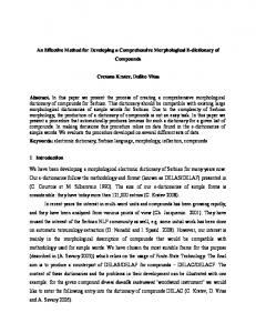
Figure 4: NDCG scores of different ranking methods for the Delicious dataset where @N denotes that the metric is evaluated only on the resources that are ranked top N in list L, r(i) is the relevance level (to be discussed shortly) of the resource ranked i in L, and ZN is a normalization factor that is chosen so that the optimal ranking’s NDCG score is 1. We invited 16 users to participate in this experiment. Each user proposed eight queries. There were thus a total of 128 unique queries. The users then determined a score for each resource returned by the ranking methods by labeling the resource with one of three relevance levels: Relevant (score 2), Partially Relevant (score 1) and Irrelevant (score 0). The overall NDCG score of a ranking method is given by the average of its NDCG scores over the 128 queries. Figures 4–6 shows the NDCG scores of the six ranking methods at different values of N for the three datasets. For CubeLSI, we set the reduction ratios c1 = c2 = c3 = 50. From the figures, we see that CubeLSI, CubeSim, and FolkRank, which use the user (tagger) dimension, consistently outperform the other three methods that consider only tags and resources. This verifies our hypothesis that incorporating tagger information in resource ranking brings about notable improvement in ranking quality. Moreover, CubeLSI gives the best ranking quality among all six ranking methods. This suggests that the three-dimensional tag semantic analysis performed by CubeLSI is very effective in distilling latent concepts from data in social tagging systems. To illustrate the quality of the ranked lists returned by CubeLSI, Table 9 in the appendix presents a few sample queries of the Delicious dataset and the top-5 resources (web sites) returned by CubeLSI for each query. To help readers understand these web sites, we show their URLs and their corresponding ODP (Open Directory Project)8 categories.

6.5

Efficiency

Having shown that CubeLSI gives the best ranking quality among the various ranking methods, our next set of experiments focuses on the efficiency aspects of CubeLSI. In particular, how it compares against the other two tagger-cognizant methods, CubeSim and FolkRank. As we have discussed, our CubeLSI approach consists of an offline pre-processing component and an online query-processing component (see Figure 1). We study these two components separately. We note that both CubeLSI and CubeSim have to pre-process the tag-assignment data and to compute pairwise tag distances for concept distillation. We will, therefore, compare CubeLSI and CubeSim in terms of pre-processing time. FolkRank, on the other hand, does not 8 http://www.dmoz.org/, by its own account, is “the largest, most comprehensive human-edited directory of the Web”.

HKUCS TR-2010-10

17

6.5

Efficiency

6


0.9 0.85

NDCG@N

0.8 0.75 0.7 0.65 0.6


0.55 0.5 0.45 0

1

2

3

4

5

6

7

8

9 10 N

15

20

Figure 5: NDCG scores of different ranking methods for the Bibsonomy dataset

0.9 0.85

NDCG@N

0.8 0.75 0.7 0.65 0.6


0.55 0.5 0.45 0

1

2

3

4

5

6

7

8

9 10 N

15

20

Figure 6: NDCG scores of different ranking methods for the Last.fm dataset

HKUCS TR-2010-10

18

6.5

Efficiency

6


Table 6: Pre-processing times (in hours) of CubeLSI and CubeSim Delicious Bibsonomy Last.fm CubeSim >100 6.29 5.50 CubeLSI 4.55 0.62 0.36 2

10

Delicious dataset Bibsonomy dataset Last.fm dataset

1

Time (h)

10

0

10

−1

10

−2

10

20 30 40 50

100 150 Reduction ratios (c1=c2=c3)

200

Figure 7: CubeLSI pre-processing time vs. reduction ratios perform much data pre-processing. Instead, FolkRank performs iterative weight propagation over a tripartite graph. (see Section 2). For CubeLSI, query processing involves computing relatively simple cosine similarity. We will compare CubeLSI and FolkRank in query-processing time. The experiments were conducted on a machine with a 2.6GHz Xeon processor with 8GB memory. We again set the reduction ratios for CubeLSI to c1 = c2 = c3 = 50. Table 6 shows the pre-processing times of CubeLSI and CubeSim over the three datasets. The pre-processing time of CubeSim on the Delicious dataset is unavailable because the computation did not finish within 100 hours. From the table, we see that CubeLSI is much faster than CubeSim in data pre-processing. The reason why CubeSim is slow is that it computes the distance between every tag pair, say ti and tj , by computing ||F:,ti ,: − F:,tj ,: ||F from the very big tensor slices (user-resource matrices) F:,ti ,: and F:,tj ,: . These tag distance computations are therefore very expensive. On the other hand, our theorems allow CubeLSI to compute tag distances from the core tensor S and the factor matrix Y (2) , which are reduced from Fˆ given the reduction ratios (c1 , c2 and c3 ). Since S and Y (2) are much smaller structures compared with the tensor slices used by CubeSim, CubeLSI compute tag distances much more efficiently. By varying the reduction ratios, CubeLSI can control the sizes of S and Y (2) , which in turn affects the pre-processing time required. Figure 7 shows the pre-processing time of CubeLSI applied on the Bibsonomy dataset at different reduction ratios. While setting appropriate values for the reduction ratios is an engineering effort, our experience with many real social tagging systems indicates that reduction ratios of around 50 strike a good balance between efficiency (pre-processing time and storage cost) and ranking result quality. Table 7 shows the total query-processing times of CubeLSI and FolkRank over the 120 queries. As we can see, CubeLSI is orders-of-magnitude faster than FolkRank in query processing. This is because FolkRank has to perform expensive iterative weight propagation over very large tripartite graphs, which includes vertices of all resources, tags, and users. For CubeLSI, only relatively simple vector dot-products are required in computing cosine similarities. Finally, we study the memory requirement of CubeLSI. Recall that the basic idea of CubeLSI ˆ is to apply Tucker decomposition on the third-order tensor F to obtain an output tensor F,

HKUCS TR-2010-10

19

REFERENCES

Table 7: Query-processing times (seconds) of CubeLSI and FolkRank Delicious Bibsonomy Last.fm FolkRank 109. 27.2 25.6 CubeLSI 0.688 1.97 0.323 Table 8: Memory requirements of Fˆ vs. S and Y (2) Delicious Bibsonomy Last.fm ˆ 7.0 TB 98 GB 88 GB F S and Y (2) 8.8 MB 3.0 MB 1.8 MB

based on which tag distances are computed. We have explained in Section 4.4 that, for a typical social tagging system, the tensor Fˆ is so huge that not even the state-of-the-art decomposition algorithm (such as MET [16]) can handle. Again, our two theorems allow CubeLSI to compute ˆ The tag distances from two relatively small structures S and Y (2) without ever materializing F. memory requirement of CubeLSI is thus much reduced. Table 8 shows the sizes of Fˆ versus the sizes of S and Y (2) for the three datasets. The table shows that our theorems lead to a very small memory requirement of CubeLSI, which is otherwise infeasible due to the gigantic storage needed.

7

Conclusion

In this paper we proposed and studied the problem of tag-based searching of resources in social tagging systems. We pointed out that, unlike traditional IR systems, social tagging systems involve casual users who label resources with descriptive tags. We observed that the involvement of causal taggers led to two distinctive properties of such systems, namely, noisy tags and multitude of aspects. To improve ranking quality, we proposed CubeLSI, a ranking algorithm that performed semantic analysis based on user/tag/resource information. CubeLSI was based on Tucker decomposition applied on a third-order tag-assignment tensor. We observed that a straightforward application of the decomposition on the tensor resulted in an output tensor that was too big to be practically useful. We proved two important theorems based on which computational shortcuts were derived to achieve very efficient tag distance computations. We showed that these distances accurately captured the semantic relationships among tags, which led to high-quality concepts. We applied CubeLSI on a number of real datasets and showed that it gave the best ranking quality compared against five other methods. Finally, we showed that CubeLSI was both computationally and storage efficient.

References [1] Benjamin Adrian, Leo Sauermann, and Thomas Roth-Berghofer. Contag: A semantic tag recommendation system. In Proceedings of I-Semantics’ 07, pages 297–304, 2007. [2] Luiz Barroso, Jeffrey Dean, and Urs Hoelzle. Web search for a planet: The Google cluster architecture. Micro, IEEE, 23(2):22–28, 2003. [3] Bin Bi, Lifeng Shang, and Ben Kao. Collaborative resource discovery in social tagging systems. In David Wai-Lok Cheung, Il-Yeol Song, Wesley W. Chu, Xiaohua Hu, and Jimmy J. Lin, editors, CIKM, pages 1919–1922. ACM, 2009. [4] Sergey Brin and Lawrence Page. The anatomy of a large-scale hypertextual web search engine. Computer Networks and ISDN Systems, 30(1–7):107–117, April 1998. [5] Alexander Budanitsky and Graeme Hirst. Evaluating wordnet-based measures of lexical semantic relatedness. Comput. Linguist., 32(1):13–47, 2006.

HKUCS TR-2010-10

20

REFERENCES

REFERENCES

[6] Chris Burges, Tal Shaked, Erin Renshaw, Ari Lazier, Matt Deeds, Nicole Hamilton, and Greg Hullender. Learning to rank using gradient descent. In ICML ’05: Proceedings of the 22nd International Conference on Machine Learning, pages 89–96, 2005. [7] Andrew Byde, Hui Wan, and Steve Cayzer. Personalized tag recommendations via tagging and content-based similarity metrics. In ICWSM ’07, 2007. [8] Hong-Ming Chen, Ming-Hsiu Chang, Ping-Chieh Chang, Ming-Chun Tien, Winston H. Hsu, and Ja-Ling Wu. Sheepdog: group and tag recommendation for Flickr photos by automatic search-based learning. In MM ’08: Proceeding of the 16th ACM International Conference on Multimedia, pages 737–740, 2008. [9] Scott Deerwester, Susan T. Dumais, George W. Furnas, Thomas K. Landauer, and Richard Harshman. Indexing by latent semantic analysis. Journal of the American Society for Information Science, 41:391–407, 1990. [10] Susan T. Dumais. Latent semantic indexing (lsi): Trec-3 report. In Overview of the Third Text REtrieval Conference, pages 219–230, 1995. [11] Nikhil Garg and Ingmar Weber. Personalized, interactive tag recommendation for Flickr. In RecSys ’08: Proceedings of the 2008 ACM conference on Recommender systems, pages 67–74, 2008. [12] Andreas Hotho, Robert Jaschke, Christoph Schmitz, and Gerd Stumme. Information retrieval in folksonomies: Search and ranking. The Semantic Web: Research and Applications, 4011:411–426, June 2006. [13] Kalervo J¨ arvelin and Jaana Kek¨ aläinen. Cumulated gain-based evaluation of IR techniques. ACM Transactions on Information Systems, 20(4):422–446, 2002. [14] Robert Jaschke, Leandro Marinho, Andreas Hotho, Lars Schmidt-Thieme, and Gerd Stumme. Tag recommendations in folksonomies. In Proceedings of the 11th European Conference on Principles and Practice of Knowledge Discovery in Databases (PKDD), pages 506–514, 2007. [15] Jay J. Jiang and David W. Conrath. Semantic similarity based on corpus statistics and lexical taxonomy. In Proceedings of the International Conference on Research in Computational Linguistics, pages 19–33, 1997. [16] Tamara G. Kolda and Jimeng Sun. Scalable tensor decompositions for multi-aspect data mining. In ICDM ’08: Proceedings of the 2008 Eighth IEEE International Conference on Data Mining, pages 363–372, 2008. [17] Yehuda Koren, Robert Bell, and Chris Volinsky. Matrix factorization techniques for recommender systems. Computer, 42(8):30–37, 2009. [18] Christian K¨ orner, Dominik Benz, Markus Strohmaier, Andreas Hotho, and Gerd Stumme. Stop thinking, start tagging: Tag semantics emerge from collaborative verbosity. In WWW ’10: Proceedings of the 19th International World Wide Web Conference, pages 521–530. ACM, 2010. [19] L. D. Lathauwer, B. D. Moor, and J. Vandewalle. A multilinear singular value decomposition. SIAM Journal on Matrix Analysis and Applications, 21(4):1253–1278, 2000. [20] L. De Lathauwer, B. De Moor, and J. Vandewalle. On the best rank-1 and rank-(r1,r2, . . . ,rn) approximation of higher-order tensors. SIAM Journal on Matrix Analysis and Applications, 21(4):1324–1342, 2000. [21] Christopher D. Manning, Prabhakar Raghavan, and Hinrich Schutze. Introduction to Information Retrieval. Cambridge University Press, 2008.

HKUCS TR-2010-10

21

REFERENCES

REFERENCES

[22] Leandro Balby Marinho and Lars Schmidt-Thieme. Collaborative tag recommendations. Proceedings of 31st Annual Conference of the Gesellschaft f¨ ur Klassifikation (GfKl) 2007, 2007. [23] Andrew Y. Ng, Michael I. Jordan, and Yair Weiss. On spectral clustering: Analysis and an algorithm. In Advances in Neural Information Processing Systems 14, pages 849–856, 2001. [24] Philip Resnik. Using information content to evaluate semantic similarity in a taxonomy. In IJCAI’95: Proceedings of the 14th international joint conference on Artificial intelligence, pages 448–453, 1995. [25] Knut Magne Risvik, Yngve Aasheim, and Mathias Lidal. Multi-tier architecture for web search engines. In LA-WEB ’03: Proceedings of the First Conference on Latin American Web Congress, page 132, 2003. [26] Ruslan Salakhutdinov and Andriy Mnih. Probabilistic matrix factorization. In NIPS ’07: Advances in Neural Information Processing Systems 20, 2007. [27] G. Salton, A. Wong, and C. S. Yang. A vector space model for automatic indexing. Commun. ACM, 18(11):613–620, 1975. [28] Borkur Sigurbjornsson and Roelof van Zwol. Flickr tag recommendation based on collective knowledge. In WWW ’08, pages 327–336, 2008. [29] G´ abor Tak´ acs, Istv´ an Pil´ aszy, Bottyán Németh, and Domonkos Tikk. Scalable collaborative filtering approaches for large recommender systems. Journal of Machine Learning Research, 10:623–656, 2009. [30] Xian Wu, Lei Zhang, and Yong Yu. Exploring social annotations for the semantic web. In Proceedings of the 15th international conference on World Wide Web, pages 417–426, 2006. [31] Zhichen Xu, Yun Fu, Jianchang Mao, and Difu Su. Towards the semantic web: Collaborative tag suggestions. In Proceedings of Collaborative Web Tagging Workshop at 15th International World Wide Web Conference, 2006.

HKUCS TR-2010-10

22

A

I3

PROOFS

… I3

…

I1 I1 I2 I2 I3 I1 I2

…

I2

I1 I3 I3 I2 I2

…

I3

…

I1

I1

Figure 8: Unfolding the tensor F ∈ RI1 ×I2 ×I3 into three matrices, F1 ∈ RI1 ×I2 I3 , F2 ∈ RI2 ×I3 I1 , and F3 ∈ RI3 ×I1 I2

A

Proofs

We first introduce the matrix unfoldings of a tensor, and then proceed to prove Theorem 1. Definition 3. The matrix unfoldings operation is the process of reordering the elements of a tensor into matrices. By performing “matrix unfoldings” on tensor F ∈ RI1 ×I2 ×I3 , we obtain three matrices F1 ∈ RI1 ×I2 I3 , F2 ∈ RI2 ×I3 I1 , and F3 ∈ RI3 ×I1 I2 . Figure 8 visualizes the unfolding processes. Intuitively, the matrix F1 is formed by cutting the tensor F along the second dimension into several “matrix slices” and listing these matrices one after another. Please refer to [19, 20] for details of the operation. Theorem 1. Let the Tucker decomposition of a third-order tensor F ∈ RI1 ×I2 ×I3 be denoted as F ≈ Fˆ = S ×1 Y (1) ×2 Y (2) ×3 Y (3)

(25)

in which Y (n) for n = 1, 2, 3 are factor matrices, and S ∈ RJ1 ×J2 ×J3 is a core tensor. Then the following holds. 12 (2) (2) (2) (2) ||Fˆ:,ti ,: − Fˆ:,tj ,: ||F = (Yti ,: − Ytj ,: )Σ(Yti ,: − Ytj ,: )T in which Σ = S2 S2T and S2 is a matrix unfolding of the core tensor S. Proof. First, we prove the following equality (2) T tr Fˆ:,ti ,: Fˆ:,t = Yti ,: Σ(Y (2) )Ttj ,: , j ,:

(26)

where tr(·) denotes the trace of matrix. From equation (25), we have (2) Fˆ:,ti ,: = S ×1 Y (1) ×2 Yti ,: ×3 Y (3) (2)

= (S ×2 Yti ,: ) ×1 Y (1) ×3 Y (3) (2)

Moreover, by the definition of the n-mode product of tensors, the product (S ×2 Yti ,: ) results in a matrix, and both Y (1) and Y (3) are matrices. It follows that (2) Fˆ:,ti ,: = Y (1) × (S ×2 Yti ,: ) × (Y (3) )T .

HKUCS TR-2010-10

23

B

ALGORITHMS

Similarly, (2) Fˆ:,tj ,: = Y (1) × (S ×2 Ytj ,: ) × (Y (3) )T .

Since the columns of factor matrices Y (n) for n = 1, 2, 3 are orthogonal, (2) (2) T T tr Fˆ:,t ,: Fˆ:,t ,: = tr (S ×2 Yt ,: )(S ×2 Yt ,: ) i

i

j

=

(2) (2) (Yti ,: S2 )(Ytj ,: S2 )T

j

(2)

= Yti ,: Σ(Y (2) )Ttj ,: .

Equality (26) holds. According to the definition of Frobenius-norm, 21 ||Fˆ:,ti ,: − Fˆ:,tj ,: ||F = tr (Fˆ:,ti ,: − Fˆ:,tj ,: )(Fˆ:,ti ,: − Fˆ:,tj ,: )T 12 T ˆ:,t ,: Fˆ T ˆ:,t ,: Fˆ T − 2tr F + tr F = tr Fˆ:,ti ,: Fˆ:,t :,tj ,: :,tj ,: i j i ,: together with the equation (26), we have 12 (2) (2) (2) (2) ||Fˆ:,ti ,: − Fˆ:,tj ,: ||F = (Yti ,: − Ytj ,: )Σ(Yti ,: − Ytj ,: )T

Theorem 2. The matrix Σ = S2 S2T in Theorem 1 is diagonal and Σi,i is the square of the ith singular value of matrix Z2 which is a matrix unfolding of tensor Z = F ×1 (Y (1) )T ×3 (Y (3) )T Proof. From equation (16), we have S:,i,: = (F ×1 (Y (1) )T ×3 (Y (3) )T ) ×2 ((Y (2) )T )i,: = Z ×2 ((Y (2) )T )i,: for 1 ≤ i ≤ J2 . Therefore, Σi,j = (S2 )i,: (S2 )Tj,: T = tr S:,i,: S:,j,: T (2) T (2) T = tr Z ×2 ((Y ) )i,: Z ×2 ((Y ) )j,: = ((Y (2) )T )i,: Z2 Z2T ((Y (2) )T )j,: Since Y (2) is the most dominant J2 singular vectors of Z2 , it follows that 0, if i 6= j Σi,j = σi2 , otherwise where σi is the ith singular value of matrix Z2 .

B

Algorithms

Algorithm 2 outlines the implementation of the alternating least squares (ALS) principle [20] for third-order tensors, which is invoked from Algorithm 1. The first step initializes factor matrices. In the second phase, based on the ALS principle [20], the factor matrices and the core tensor are iteratively adjusted until kSkT ceases to increase. In the algorithm, the function call SVD(M ) returns 3 matrices (U, V, W ) that constitute a singular value decomposition of M with the property M = U V W T . The function call unfold(n, X ) returns the matrix unfolding Xn of X .

HKUCS TR-2010-10

24

B

ALGORITHMS

Algorithm 2: ALS Input: tensor F ∈ RI1 ×I2 ×I3 , target core tensor dimensions J1 , J2 , J3 Output: core tensor S, factor matrices Y (1) , Y (2) , Y (3) , temporary matrix Λ2 for n = 2, 3 do // Initialization (Un , Λn , VnT ) ← SVD(unfold(n, F )) Y (n) ← most dominant Jn singular vectors of Un end repeat for (i, j, k) = (1, 2, 3), (3, 1, 2), (2, 3, 1) do Z ← F ×j (Y (j) )T ×k (Y (k) )T (Ui , Λi , ViT ) ← SVD(unfold(i, Z)) Y (i) ← most dominant Ji singular vectors of Ui end S ← Z ×2 (Y (2) )T until kSkT does not increase return (S, Y (1) , Y (2) , Y (3) , Λ2 )

HKUCS TR-2010-10

25

B

Queries

ALGORITHMS

Table 9: Samples of search results produced by our approach Top-5 Relevant URLs ODP Categories top/shopping/classifieds/automotive

car, shopping

http://www.cars.com/

top/regional/north america/united states/illinois/ localities/c/chicago/business and economy/automotive

http://www.kbb.com/

top/home/consumer information/automobiles/ purchasing

http://www.nadaguides.com/


http://www.carbuyingtips.com/


http://www.autobytel.com/ http://www.securityfocus.com/ https://grc.com/x/ne.dll?bh0bkyd2 network, security

http://www.ethereal.com/

top/computers/security/news and media top/computers/hacking/exploits top/computers/security/internet/services top/computers/software/operating systems/linux/ projects/networking top/computers/software/operating systems/linux/ projects/security

http://www.bleedingsnort.com/ http://www.nanog.org/ http://nugs.net/ mp3, radio, music, online

top/shopping/vehicles/autos/buyer services

top/computers/security/intrusion detection systems/ products and tools/open source top/computers/internet/organizations/internet backbone top/arts/music/styles/r/rock/jam/mp3 top/arts/music/concerts and events/internet broadcasts top/arts/music/sound files/mp3

http://www.soundclick.com/

top/arts/music/sound files/asf top/business/arts and entertainment/music/ production/m

http://www.radiolovers.com/

top/arts/radio/formats/old-time radio/ streaming mp3 stations

http://www.kurthanson.com/ http://www.dxtuners.com/

top/computers/internet/broadcasting/information

http://www.mediamonkey.com/

top/recreation/radio/shortwave and dx listening top/computers/multimedia/music and audio/ audio formats/mp3/software/all-in-one top/computers/multimedia/music and audio/ audio formats/mpeg-4/software

http://www.audiograbber.com-us.net/

top/computers/multimedia/music and audio/ audio formats/mp3/software/rippers top/computers/software/shareware/windows/ multimedia/music and audio/mp3/rippers

download, software, mp3

top/computers/multimedia/music and audio/ audio formats/mpeg-4/software top/computers/multimedia/music and audio/ audio formats/mod/software

http://www.winamp.com/

top/computers/multimedia/music and audio/ audio formats/mp3/software/players top/computers/multimedia/music and audio/ audio formats/mp3/software/all-in-one top/computers/software/shareware/windows/ multimedia/music and audio/players

http://www.mp3000.net/ http://www.emp3world.com/

HKUCS TR-2010-10

top/arts/music/sound files/mp3/search engines top/arts/music/sound files/mp3/search engines top/arts/music/sound files/mp3/downloads

26