Cubic B-Spline Curves with Shape Parameter and Their Applications

Hindawi Mathematical Problems in Engineering Volume 2017, Article ID 3962617, 7 pages https://doi.org/10.1155/2017/3962617

Research Article Cubic B-Spline Curves with Shape Parameter and Their Applications Houjun Hang, Xing Yao, Qingqing Li, and Michel Artiles School of Mathematics and Computer Science, Anhui Normal University, Wuhu 241000, China Correspondence should be addressed to Houjun Hang; [email protected] Received 4 July 2017; Accepted 26 November 2017; Published 17 December 2017 Academic Editor: Giovanni Garcea Copyright © 2017 Houjun Hang et al. This is an open access article distributed under the Creative Commons Attribution License, which permits unrestricted use, distribution, and reproduction in any medium, provided the original work is properly cited. The present studies on the extension of B-spline mainly focus on Bezier methods and uniform B-spline and are confined to the adjustment role of shape parameters to curves. Researchers pay little attention to nonuniform B-spline. This paper discusses deeply the extension of the quasi-uniform B-spline curves. Firstly, by introducing shape parameters in the basis function, the spline curves are defined in matrix form. Secondly, the application of the shape parameter in shape design is analyzed deeply. With shape parameters, we get another means for adjusting the curves. Meanwhile, some examples are given. Thirdly, we discuss the smooth connection between adjacent B-spline segments in detail and present the adjusting methods. Without moving the control points position, through assigning appropriate value to the shape parameter, C1 continuity of combined spline curves can be realized easily. Results show that the methods are simple and suitable for the engineering application.

1. Introduction B-spline methods are very popular in computer-aided geometric design and associated fields because of their distinct advantages. In recent years, some other methods have been presented for representing curves and surfaces. Papers [1–7] presented successively C-curves, T-curves, TC-curves, and 𝛽spline in trigonometric functions space. In order to improve the flexibility of product design, researchers give further consideration to introduce shape parameters. Through the parameters, designers can adjust flexibly the shape of curves and surfaces. Wang et al. [8, 9] introduced successively shape parameters to uniform quadratic TC-B-spline curves and quadratic TC-Bezier curves. Xiong et al. [10] discussed extension of uniform C-B-spline curves and surfaces. Bashir et al. [11] researched the G2 and C2 rational quadratic trigonometric Bezier curve with two shape parameters, and Liu et al. [12] discussed further hyperbolic polynomial uniform B-spline curves and surfaces with shape parameter. In recent years, researchers also paid attention to extension of traditional B-spline methods. But they mainly concentrated on Bezier curves [13], quadratic and cubic uniform B-spline curves [14–19]. Uniform B-splines can represent overall continuity closed curves and surfaces. But they use equally spaced knots;

the spline does not interpolate the first and last control points. Because a nonuniform B-spline uses repeated knots technology, the curves have clamped property. The designers can locate more easily the two end points of the curve and achieve smooth connection between adjacent B-spline segments. So it has more practical significance for us to study extension of nonuniform B-spline curves and surfaces. This paper discusses mainly cubic B-spline curves with shape parameter and presents the matrix representation and analyzes the influence of shape parameter on the curve shape. The application of the shape parameter in shape design is discussed deeply. With shape parameters, we get another means for adjusting the curves. In the end, we focus on discussions about how to realize C1 continuity between adjacent B-spline segments by only adjusting the value of the shape parameters without changing the position of the control points. Results show that the methods given by this paper are simple and suitable for the engineering application.

2. Definition of Basis Functions and Curves Given control points 𝑑0 , 𝑑1 , . . . , 𝑑𝑛 , let the knot vector be U = [0, 0, 0, 1, 2, . . . , 𝑛 − 2, 𝑛 − 1, 𝑛 − 1, 𝑛 − 1]. Then we have

2

Mathematical Problems in Engineering 1

(2) When 𝑛 = 3, the spline curve is composed of two segments.

0.9 0.8

2

1 p1 (𝑡) = ∑ 𝑑𝑗 𝑁𝑗,2 (𝜆, 𝑡) ,

0.7 0.6

𝑗=0

0.5

3

(5)

2 p2 (𝑡) = ∑ 𝑑𝑗 𝑁𝑗,2 (𝜆, 𝑡) ,

0.4

𝑗=1

0.3 0.2

𝑡 ∈ [0, 1]

0.1 0

0

0.1

0.2

0.3

0.4

0.5

0.6

0.7

0.8

0.9

1 𝑁0,2 (𝜆, 𝑡) = (1 + 𝜆𝑡) (1 − 𝑡)2 ,

1

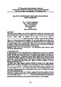
Figure 1: The influence of the parameter on the spline shape (𝑛 = 2).

1 𝑁1,2 (𝜆, 𝑡) =

1 (2 + 𝜆𝑡) (2 − 𝑡) 𝑡 4 + (1 − 𝜆 (1 − 𝑡)) 𝑡 (1 − 𝑡) ,

a piecewise representation of the quadratic open uniform Bspline with parameter 𝑖

p (𝑢) = ∑ d𝑗 𝑁𝑗,2 (𝜆, 𝑢) ,

(1)

𝑗=𝑖−2

𝑢 ∈ [𝑖, 𝑖 + 1] ⊂ [0, 𝑛 − 1] , 𝑖 = 2, 3, . . . , 𝑛, where −1 ≤ 𝜆 ≤ 1 is called shape parameter and 𝑁𝑗,2 (𝜆, 𝑢) (𝑗 = 0, 1, . . . , 𝑛) are basis functions. (1) When 𝑛 = 2, the curve only has one segment.

1 𝑁2,2 (𝜆, 𝑡) =

1 (2 (1 − 𝜆) + 𝜆𝑡) 𝑡2 , 4

2 𝑁1,2 (𝜆, 𝑡) =

1 (2 + 𝜆 + 𝜆𝑡) (1 − 𝑡)2 , 4

2 𝑁2,2 (𝜆, 𝑡) =

1 (2 − 𝜆 (1 − 𝑡)) (1 − 𝑡) (1 + 𝑡) 4

(6)

(7)

+ (1 + 𝜆𝑡) 𝑡 (1 − 𝑡) , 2 𝑁3,2 (𝜆, 𝑡) = (𝜆𝑡 − 𝜆 + 1) 𝑡2 .

Also it can be expressed in the following matrix form: 2

0 p (𝑡) = ∑ d𝑗 𝑁𝑗,2 (𝜆, 𝑡) ,

𝑡 ∈ [0, 1] ,

d0

(2)

𝑗=0

2

3

p1 (𝑡) = [1 𝑡 𝑡 𝑡 ] 𝑀1 (𝜆) (d1 ) , 𝑡 ∈ [0, 1] ,

0 0 0 where 𝑁0,2 (𝜆, 𝑡), 𝑁1,2 (𝜆, 𝑡), and 𝑁2,2 (𝜆, 𝑡) are

d2 1

0 𝑁0,2 (𝜆, 𝑡) = (1 + 𝜆𝑡) (1 − 𝑡)2 , 0 𝑁1,2

(𝜆, 𝑡) = (2 − 𝜆 + 2𝜆𝑡) (1 − 𝑡) 𝑡,

(3)

0 𝑁2,2 (𝜆, 𝑡) = (1 − 𝜆 + 𝜆𝑡) 𝑡2 .

Also it can be expressed in matrix form:

0

(4)

−2 (1 + 𝜆) 2 − 𝜆 0 ). 𝑀=( 1+𝜆 3𝜆 − 2 1 − 𝜆 −2𝜆

(8)

d3

d2

0

𝜆−2 2−𝜆 0 ( ) 5 3 1 𝑀1 = ( ), 1 − 2𝜆 𝜆 − (1 − 𝜆) 2 2 2 5 1 𝜆 − 𝜆 𝜆 4 4 ( ) p2 (𝑡) = [1 𝑡 𝑡2 𝑡3 ] 𝑀2 (𝜆) (d2 ) , 𝑡 ∈ [0, 1] ,

p (𝑡) = [1 𝑡 𝑡2 𝑡3 ] 𝑀 (𝜆) (d1 ) , 𝑡 ∈ [0, 1] , 0

0

d1

d0

1+𝜆

0

𝜆

Figure 1 shows the influence of the parameter 𝜆 on 𝑁0,2 (𝜆, 𝑢), 𝑁1,2 (𝜆, 𝑢), and 𝑁2,2 (𝜆, 𝑢), where solid line, dash line, and dotted line correspond to 𝜆 = 1, 𝜆 − 1, and 𝜆 = 0.

1 1 1 + 𝜆 (2 − 𝜆) 0 2 4 4 1 1 0 ) (−1 − 4 𝜆 1 + 4 𝜆 ). 𝑀2 = ( (1 1 ) 5 3 − 𝜆 𝜆− 1−𝜆 2 4 4 2 1 5 𝜆 − 𝜆 𝜆 ( 4 ) 4 Figure 2 shows the influence of 𝜆 on the shape of 𝑁0,2 (𝜆, 𝑢), 𝑁1,2 (𝜆, 𝑢), 𝑁2,2 (𝜆, 𝑢), and 𝑁3,2 (𝜆, 𝑢), where solid line and dash line correspond to 𝜆 = 0.6 and 𝜆 = −0.5.

Mathematical Problems in Engineering

3

1

1

0.9

0.9

0.8

0.8

0.7

0.7

0.6

0.6

0.5

0.5

0.4

0.4

0.3

0.3

0.2

0.2

0.1

0.1

0

0

0.2

0.4

0.6

0.8

1

1.2

1.4

1.6

1.8

0

2

0

0.5

1

1.5

2

2.5

3

3.5

4



(3) When 𝑛 > 3, the spline curve is composed of 𝑛 − 1 segments.

Also it can be expressed in the following matrix form:

p1 (𝑡) =

2

1 ∑ 𝑑𝑗 𝑁𝑗,2 𝑗=0

d𝑛−2 p𝑛−1 (𝑡) = [1 𝑡 𝑡2 𝑡3 ] 𝑀𝑛−1 (𝜆) (d𝑛−1 ) , d𝑛

(𝜆, 𝑡) ,

𝑛

𝑛−1 p𝑛−1 (𝑡) = ∑ d𝑗 𝑁𝑗,2 (𝜆, 𝑡) , 𝑗=𝑛−2

(9) 𝑀𝑛−1

𝑖

3 pi−1 (𝑡) = ∑ 𝑑𝑗 𝑁𝑗,2 (𝜆, 𝑡) , 𝑖 = 3, . . . , 𝑛 − 1, 𝑗=𝑖−2

𝑡 ∈ [0, 1] , where

1 𝑁0,2 ,

1 𝑁1,2 ,

𝑛−1 𝑁𝑛−2,2 (𝜆, 𝑡) = 𝑛−1 𝑁𝑛−1,2

and

1 𝑁2,2

1 (2 + 𝜆 + 𝜆𝑡) (1 − 𝑡)2 , 4

1 (𝜆, 𝑡) = (2 − 𝜆 (1 − 𝑡)) (1 − 𝑡) (1 + 𝑡) 4 𝑀𝑖−1

+ (1 + 𝜆𝑡) 𝑡 (1 − 𝑡) , 𝑛−1 𝑁𝑛,2 (𝜆, 𝑡) = (𝜆𝑡 − 𝜆 + 1) 𝑡2 ,

1 (2 + 𝜆 + 𝜆𝑡) (1 − 𝑡)2 , 4

3 𝑁𝑖−1,2 (𝜆, 𝑡) =

1 (2 − 𝜆 (1 − 𝑡)) (1 − 𝑡) (1 + 𝑡) 4 +

3 𝑁𝑖,2 (𝜆, 𝑡) =

1 (2 + 𝜆𝑡) 𝑡 (2 − 𝑡) , 4

1 (𝜆𝑡 − 2𝜆 + 2) 𝑡2 , 4

(11)

d𝑖−2 2 3 p𝑖−1 (𝑡) = [1 𝑡 𝑡 𝑡 ] 𝑀𝑖−1 (𝜆) (d𝑖−1 ) , d𝑖

are shown in (6).

3 𝑁𝑖−2,2 (𝜆, 𝑡) =

1 1 1 + 𝜆 (2 − 𝜆) 0 2 4 4 (−1 − 1 𝜆 1 + 1 𝜆 0 ) ( ) 4 4 ), =( (1 1 ) ( − 𝜆 5 𝜆 − 3 1 − 𝜆) 2 4 4 2 1 5 𝜆 − 𝜆 𝜆 ( 4 ) 4

(10)

1 1 0 (2 + 𝜆) (2 − 𝜆) 4 4 1 1 (− (4 + 𝜆) ) 0 (4 + 𝜆) ( 4 ) 4 =( ). ( 1 ) 1 1 (2 − 𝜆) (−4 + 3𝜆) (1 − 𝜆) 4 4 2 1 1 1 𝜆 − 𝜆 𝜆 ( ) 4 2 4

Figure 3 shows the influence of the parameter 𝜆 on the shape of basis functions 𝑁0,2 (𝜆, 𝑢), 𝑁1,2 (𝜆, 𝑢), 𝑁2,2 (𝜆, 𝑢), 𝑁3,2 (𝜆, 𝑢), 𝑁4,2 (𝜆, 𝑢), and 𝑁5,2 (𝜆, 𝑢), where solid line and dash line correspond to 𝜆 = 0.5 and 𝜆 = −0.7.

3. The Properties of Basis Functions and Spline Curves (1)

𝑖 = 3, 4, . . . , 𝑛 − 1.

𝑗

𝑁𝑖 (𝜆, 𝑢) ≥ 0,

∀𝑢 ∈ [0, 1] , 𝜆 ∈ [−1, 1] .

(12)

4

Mathematical Problems in Engineering 2

(2)

1.8

2

0 ∑ 𝑁𝑗,2 (𝜆, 𝑢) = 1,

1.6

𝑗=0

1.4

2

1.2

1 ∑ 𝑁𝑗,2 (𝜆, 𝑢) = 1,

1

𝑗=0

0.8

3

2 ∑ 𝑁𝑗,2 (𝜆, 𝑢) = 1,

0.6

(13)

0.4

𝑗=1

0.2

𝑛

𝑛−1 ∑ 𝑁𝑗,2 (𝜆, 𝑢) = 1

0 −3

𝑗=𝑛−2 𝑖

3 ∑ 𝑁𝑗,2 (𝜆, 𝑢) = 1,

−2

0

−1

1

2

3

Figure 4: 𝛼 = −0.65, 0, and 0.65 corresponded, respectively, to the thick line, the thin line, and the dash line.

𝑖 = 3, 4, . . . , 𝑛 − 1.

𝑗=𝑖−2

5

(3)

d5

4.5

1 𝑡=0 { { { { 𝑗 𝑁0,2 (𝜆, 𝑡) {> 0 𝑡 ∈ (0, 1) { { { 𝑡 = 1, {0

y

𝑗 = 0, 1,

0 𝑁2,2

0 𝑡=0 { { { { (𝜆, 𝑡) {> 0 𝑡 ∈ (0, 1) { { { 𝑡 = 1, {1

(14)

d2

d4

1.5 0.5

d0 1

1.5

2

2.5

3

3.5

4

4.5

5

5.5

6

6.5

x

(6) 1 p󸀠𝑖−1 (𝜆, 1) = (1 − 𝜆) (d𝑖 − d𝑖−1 ) , 4 1 p󸀠𝑖 (𝜆, 0) = (1 + 𝜆) (d𝑖 − d𝑖−1 ) , 4

(17)

𝑖 = 2, 3, . . . , 𝑛 − 2. That is to say, the curve is G1 at inner knots. Especially when 𝜆 = 0, the curve is C1. (15)

4. Application in Shape Design

(5) 𝑑p1 󵄨󵄨󵄨󵄨 𝑑p 󵄨󵄨󵄨󵄨 󵄨󵄨 = 󵄨 = (2 − 𝜆) (d1 − d0 ) , 𝑑𝑢 󵄨󵄨𝑢=0 𝑑𝑡 󵄨󵄨󵄨𝑡=0 𝑑p𝑛−1 󵄨󵄨󵄨󵄨 𝑑p 󵄨󵄨󵄨󵄨 = 󵄨󵄨 󵄨 = (2 + 𝜆) (d𝑛 − d𝑛−1 ) . 𝑑𝑢 󵄨󵄨𝑢=𝑛−1 𝑑𝑡 󵄨󵄨󵄨𝑡=1

3

Figure 5: 𝜆 = 0.5 corresponds to the solid line and 𝜆 = −0.4 the dash line.

where 𝜆 = 0, that is, quadratic open B-spline. (4)

p (𝑛 − 1) = d𝑛 .

3.5

2

0 𝑡=0 { { { { (𝜆, 𝑡) {> 0 𝑡 ∈ (0, 1) { { { 𝑡 = 1, {1

p (0) = d0 ,

d3

2.5

0 𝑡=0 { { { { 2 𝑁3,2 (𝜆, 𝑡) {> 0 𝑡 ∈ (0, 1) { { { 𝑡 = 1, {1 𝑛−1 𝑁𝑛,2

d1

4

(16)

Nonuniform B-spline methods have important applications in shape design. By modifying the shape parameters, the designers get additional choice in two-dimensional design. Figures 4–6 illustrate the influence of the parameter 𝜆 on the shape of curve, where Figure 4 shows 𝛼 = −0.65, 0, and 0.65 corresponding, respectively, to the thick line, the thin line, and the dash line. Figure 5 shows 𝜆 = 0.5 corresponding


5

2.5 2 1.5 1 0.5 0 −0.5 −1 −1.5 −2

−1.5

−1

−0.5

0

0.5

1

1.5

2

Figure 6: 𝛼 = −0.4, 0, and 0.4 corresponded, respectively, to the solid line, the dotted line, and the dash line.

Figure 9: Fractal curve generated by the spline curve in this paper (𝛼 = −0.55).

Figure 7: Fractal curve generated by the spline curve in this paper (𝛼 = −0.6, 4 iterations).

Figure 8: Fractal curve generated by the spline curve in this paper (𝛼 = −0.6, 5 iterations).

to the solid line and 𝜆 = −0.4 the dash line. Figure 6 shows 𝛼 = −0.4, 0, and 0.4 corresponding, respectively, to the solid line, the dotted line, and the dash line. Figures 7–11 show the application of the spline cure in this paper in fractal modeling.

Figure 10: Fractal curve generated by the spline curve in this paper (𝛼 = −0.8).

5. Composite Spline Curves In the practical application, we usually construct composite spline curves that satisfy some smooth conditions. By adjusting shape parameters, designers can achieve the goal. Two spline curves are given: The first one is 𝑖

p (𝑢) = ∑ p𝑗 𝑁𝑗,2 (𝜆 1 , 𝑢) , 𝑗=𝑖−2

(18)

𝑢 ∈ [𝑖 − 2, 𝑖 − 1] ⊂ [0, 𝑛 − 1] , 𝑖 = 2, 3, . . . , 𝑛, 𝜆 1 ∈ [−1, 1] .

The knot vector U = [0, 0, 0, 1, 2, . . . , 𝑛 − 2, 𝑛 − 1, 𝑛 − 1, 𝑛 − 1].

Figure 11: Fractal curve generated by the spline curve in this paper (𝛼 = 0).

6

Mathematical Problems in Engineering 2.6

The second one is

2.4

𝑖

q (𝑢) = ∑ q𝑗 𝑁𝑗,2 (𝜆 2 , V) ,

(19)

𝑗=𝑖−2

V ∈ [𝑖 − 2, 𝑖 − 1] ⊂ [0, 𝑚 − 1] , 𝑖 = 2, 3, . . . , 𝑚, 𝜆 2 ∈ [−1, 1] .

The knot vector V = [0, 0, 0, 1, 2, . . . , 𝑚−2, 𝑚−1, 𝑚−1, 𝑚−1]. From the equations above, p𝑛 ≡ q0 . If curves p(𝑡) and q(𝑡) satisfy G1 continuity that ∃𝛿 > 0, Δq0 = 𝛿p𝑛−1 , we can modify the parameter to enable the two curves’ C1 continuity without changing the position of the control points. The adjusting methods are shown below. (1) If [2 − 3/𝛿, 2 − 1/𝛿] ∩ [−1, 1] ≠ Φ, we choose 𝜆 2 ∈ [2 − 3/𝛿, 2 − 1/𝛿] ∩ [−1, 1] and modify 𝜆 1 = (2 − 𝜆 2 )𝛿 − 2. (2) If [𝛿 − 2, 3𝛿 − 2] ∩ [−1, 1] ≠ Φ, we choose 𝜆 1 ∈ [𝛿 − 2, 3𝛿 − 2] ∩ [−1, 1] and adjust 𝜆 2 = 2 − (2 + 𝜆 1 )/𝛿. We only prove that (1) and (2) can be gotten in the same way. If [2 − 3/𝛿, 2 − 1/𝛿] ∩ [−1, 1] ≠ Φ, we can choose freely the value of 𝜆 2 as long as 𝜆 2 ∈ [2 − 3/𝛿, 2 − 1/𝛿] ∩ [−1, 1]. From 2 − 3/𝛿 ≤ 𝜆 2 ≤ 2 − 1/𝛿, we find −1 ≤ (2 − 𝜆 2 )𝛿 − 2 ≤ 1 and adjust 𝜆 1 = (2 − 𝜆 2 )𝛿 − 2. 𝑑q 󵄨󵄨󵄨󵄨 󵄨 = (2 − 𝜆 2 ) (Q1 − Q0 ) 𝑑V 󵄨󵄨󵄨V=0 = (2 − 𝜆 2 ) 𝛿 (p𝑛 − p𝑛−1 ) ,

(20)

𝑑p 󵄨󵄨󵄨󵄨 = (2 + 𝜆 1 ) (p𝑛 − p𝑛−1 ) . 󵄨 𝑑𝑢 󵄨󵄨󵄨𝑢=𝑛−1 From 𝜆 1 = (2 − 𝜆 2 )𝛿 − 2, we find 𝛿 = (2 + 𝜆 1 )/(2 − 𝜆 2 ). So (𝑑q/𝑑V)|V=0 = (𝑑p/𝑑𝑢)|𝑢=𝑛−1 . Two spline curves are given. The first one is p(𝑢) = ∑5𝑗=0 p𝑗 𝑁𝑗,2 (𝜆 1 , 𝑢) =

∑𝑖𝑗=𝑖−2 p𝑗 𝑁𝑗,2 (𝜆 1 , 𝑢), 𝑢 ∈ [𝑖 − 2, 𝑖 − 1] ⊂ [0, 4], 𝑖 = 2, 3, 4, 5, 𝜆 1 ∈ [−1, 1]. The knot vector U = [0, 0, 0, 1, 2, 3, 4, 4, 4]. The second one is q(𝑢) = ∑4𝑗=0 q𝑗 𝑁𝑗,2 (𝜆 2 , V) = ∑𝑖𝑗=𝑖−2 q𝑗 𝑁𝑗,2 (𝜆 2 , V), V ∈ [𝑖−2, 𝑖−1] ⊂ [0, 3], 𝑖 = 2, 3, 4, 𝜆 2 ∈ [−1, 1]. The knot vector V = [0, 0, 0, 1, 2, 3, 3, 3], where 𝜆 1 = 0.6 and 𝜆 2 = 0.4 and the control points are p0 (0.5, 1) , p1 (1, 2) , p2 (2, 2.25) , p3 (3, 1.5) , p4 (4, 2.25) , p5 (5, 1.25) q0 (5, 1.25) ,

(21)

2.2 2 1.8 1.6 1.4 1.2 1 0.8 0.6

0

1

2

3

4

5

6

7

8

1

Figure 12: C composite spline curve.

Looking at the control points, we see that p5 ≡ q0 and Δq0 = 𝛿p4 , 𝛿 = 1/2. Because [2 − 3/𝛿, 2 − 1/𝛿] ∩ [−1, 1] = [−4, 0] ∩ [−1, 1] ≠ Φ, we can choose 𝜆 2 ∈ [−4, 0] ∩ [−1, 1]. Here we let 𝜆 2 = −0.5. From the above method, we adjust 𝜆 1 = 0.6 to 𝜆 1 = (2−𝜆 2 )𝛿− 2 = −0.75. Now, the curves p(𝑡) and q(𝑡) are of C1 continuity, as shown in Figure 12, where the solid line is 𝑡, the original curve, and the dash line is the adjusted curve. On one hand, the adjusting methods are very simple to do, as shown in (1) and (2) in Section 5. On the other hand, the adjusting methods let the designers achieve easily smooth connection between adjacent B-spline segments without moving the control points. So it is suitable for the engineering application.

6. Conclusion This paper proposes a class of cubic spline curves with parameter. It is actually the extension of quadratic open Bspline. Through the parameter, we can adjust flexibly the shape of spline curves. With different parameter values, the curve is dragged near or pushed away from the curve. The spline curve is global G1 and keeps clamped property. We can realize C1 smooth connection between the spline curves by only modifying the shape parameter value without changing the control points. The adjusting methods proposed in this paper have very important application value.

Conflicts of Interest The authors declare that they have no conflicts of interest.

q1 (5.5, 0.75) , q2 (6.5, 2) , q3 (7, 1) , q4 (8, 2.5) .

Acknowledgments This work has been supported by the Provincial Natural Science Research Project of Anhui Colleges under Grant no. KJ2017A326.


References [1] J. Zhang, “Two different forms of C-B-splines,” Computer Aided Geometric Design, vol. 14, no. 1, pp. 31–41, 1997. [2] J. Zhang, “C-Bezier curves and surfaces,” CVGIP: Graphical Models and Image Processing, vol. 61, no. 1, pp. 2–15, 1999. [3] B. A. Barsky, Computer Graphics and Geometric Modeling Using Beta-Spline, Computer Science Workbench, Springer-Verlag, Berlin, Heidelberg, Germany, 1988. [4] B. Joe, “Multiple-Knot and Rational Cubic Beta-Splines,” ACM Transactions on Graphics, vol. 8, no. 2, pp. 100–120, 1989. [5] J. Zhang, “C-curves: an extension of cubic curves,” Computer Aided Geometric Design, vol. 13, no. 3, pp. 199–217, 1996. [6] M. Ding and G. Z. Wang, “T-B´ezier Curves Based on Algebraic and Trigonometric Polynomials,” Chinese Journal of Computers, vol. 27, no. 8, pp. 1021–1026, 2004. [7] E. J. Evans, M. A. Scott, X. Li, and D. C. Thomas, “Hierarchical T-splines:Analysis-suitability,Bezier extraction, and application as an adaptive basis for isogeometric analysis,” Computer Methods Applied Mechanics and Engineering, vol. 284, pp. 1–20, 2015. [8] L. Wang and X. Liu, “Quadratic TC-Bezier Curves with Shape Paramrters,” Computer Engineering and Design, vol. 28, no. 5, pp. 1096-1097, 2007. [9] S. Ma, “Extention of Quadratic Uniform TC-B Spline curves and Surfaces,” Computer Engineering and Design, vol. 29, pp. 5863–5865, 2008. [10] J. Xiong, Q. Guo, and G. Zhu, “Extension of Uniform C-B Spline curves and Surfaces,” Computer Engineering and Design, vol. 29, no. 23, pp. 6102–6104, 2008. [11] U. Bashir, M. Abbas, and J. M. Ali, “The G2 and C2 rational quadratic trigonometric B´ezier curve with two shape parameters with applications,” Applied Mathematics and Computation, vol. 219, no. 20, pp. 10183–10197, 2013. [12] X. Liu, W. Xu, Y. Guan, and Y. Shang, “Hyperbolic polynomial uniform B-spline curves and surfaces with shape parameter,” Graphical Models, vol. 72, no. 1, pp. 1–6, 2010. [13] X. Qin, G. Hu, N. Zhang, X. Shen, and Y. Yang, “A novel extension to the polynomial basis functions describing Bezier curves and surfaces of degree n with multiple shape parameters,” Applied Mathematics and Computation, vol. 223, pp. 1–16, 2013. [14] G. Liu and J. Tan, “Extension of the uniform quadratic B-spline curves,” Journal of Hefei University of Technology, vol. 27, no. 5, pp. 459–462, 2004. [15] S. Tao, “Extension of the uniform quadratic B-spline curves,” Computer Aided Engineering, vol. 16, no. 2, pp. 54–56, 2008. [16] C. Xia and H. Wu, “Extension of Uniform Cubic B-Spline Curves with Multiple Shape Parameters,” Journal of Engineering Graphics, vol. 32, no. 2, pp. 73–79, 2011. [17] J. Zhang and Z. Gen, “𝛼 Extension of the Cubic Uniform BSpline Curve,” Journal of Computer-Aided Design and Computer Graphics, vol. 19, no. 7, pp. 884–887, 2007. [18] J. Cao and G. Wang, “The structure of uniform B-spline curves with parameters,” Progress in Natural Science, vol. 18, no. 3, pp. 303–308, 2008. [19] G. Hu and X. Qin, “The construction of 𝜆𝜇-B-spline curves and its application to rotational surfaces,” Applied Mathematics and Computation, vol. 266, pp. 194–211, 2015.

7

Advances in

Operations Research Hindawi Publishing Corporation http://www.hindawi.com

Volume 2014

Advances in

Decision Sciences Hindawi Publishing Corporation http://www.hindawi.com

Volume 2014

Journal of

Applied Mathematics

Algebra

Hindawi Publishing Corporation http://www.hindawi.com


Volume 2014

Journal of

Probability and Statistics Volume 2014

The Scientific World Journal Hindawi Publishing Corporation http://www.hindawi.com


Volume 2014

International Journal of

Differential Equations Hindawi Publishing Corporation http://www.hindawi.com

Volume 2014

Volume 2014

Submit your manuscripts at https://www.hindawi.com International Journal of

Advances in

Combinatorics Hindawi Publishing Corporation http://www.hindawi.com

Mathematical Physics Hindawi Publishing Corporation http://www.hindawi.com

Volume 2014

Journal of

Complex Analysis Hindawi Publishing Corporation http://www.hindawi.com

Volume 2014

International Journal of Mathematics and Mathematical Sciences


Journal of

Mathematics Hindawi Publishing Corporation http://www.hindawi.com

Volume 2014


Volume 2014

Volume 2014


Volume 2014

#HRBQDSDĮ,@SGDL@SHBR

Journal of

Volume 201


Discrete Dynamics in Nature and Society

Journal of

Function Spaces Hindawi Publishing Corporation http://www.hindawi.com

Abstract and Applied Analysis

Volume 2014


Volume 2014


Volume 2014

International Journal of

Journal of

Stochastic Analysis

Optimization



Volume 2014

Volume 2014