Jan 18, 2010 - This technical report will detail the activities of the Curiosity Cloning project conducted at Dublin ... 20. 5 Signal Processing, Feature Extraction and Machine Learning. 24 ... Examples of an oddball (a) and non-oddball (b) images from the Simu- ..... oped for the subjects to drive the pace of the experiment.
Curiosity Cloning: Neural Modelling for Image Analysis, Technical Report Graham Healy1 , Peter Wilkins1 , Alan F. Smeaton1 Dario Izzo2 , Christos Ampatzis2 , Marek Rucinski2 , Eduardo Martin Moraud2 1 CLARITY: Centre for Sensor Web Technologies, Dublin City University, Ireland 2 Advanced Concepts Team (ACT), European Space and Technology Research Center (ESTEC), The Netherlands January 18, 2010 Abstract This technical report will detail the activities of the Curiosity Cloning project conducted at Dublin City University (DCU) in conjunction with the Advanced Concepts Team (ACT), funded through the European Space Agencies (ESA) Ariadna scheme. The primary objective of this project was the utilization of a cheap, commodity Electroencephalography (EEG) device which has only four nodes, to the application of ‘oddball’ style, visual RSVP experiments. During this project we determined that it was indeed possible to employ such a device which captured sufficient information that discriminative classifiers were able to be constructed, which for a given subject, were able to classify that subjects stimuli response into either oddball or non-oddball events, at speeds of up to 50 milliseconds. Furthermore, in this project we pushed beyond the binary class distinction of oddball versus nonoddball, and introduced a third type, the non-obvious oddball. This class of oddball was designed such that it enabled the capture of data from an ‘expert’ subject, as to what they found ‘interesting’ in a series of presented stimuli. Our experiments demonstrate that there is some applicability to this, and warrants continued investigation.
1
Contents 1 Background
5
2 Motivation
7
3 Experimental Setup 3.1 Apparatus . . . . . . . . . . . . . . . . . . . . . . 3.2 Subjects . . . . . . . . . . . . . . . . . . . . . . . 3.3 Experiment Methodology . . . . . . . . . . . . . 3.4 Data Collections and Associated Experiments . . 3.4.1 Collection 1: Simulated Martian Rocks . . 3.4.2 Collection 2: Optimization Visualizations 3.4.3 Collection 3: SenseCam . . . . . . . . . .
. . . . . . .
. . . . . . .
. . . . . . .
. . . . . . .
. . . . . . .
. . . . . . .
. . . . . . .
. . . . . . .
. . . . . . .
. . . . . . .
. . . . . . .
. . . . . . .
. . . . . . .
. . . . . . .
4 Event Related Potential (ERP)
8 8 12 13 13 13 16 19 20
5 Signal Processing, Feature Extraction and Machine Learning 24 5.1 Classifier Construction . . . . . . . . . . . . . . . . . . . . . . . . . . . . . 26 6 Experimental Results 6.1 Evaluation Methodology . . . . . 6.2 Experiment 2 . . . . . . . . . . . 6.3 Experiment 3 and Experiment 4 6.4 Experiment 5 . . . . . . . . . . . 6.5 Experiment 6 . . . . . . . . . . . 6.6 Experiment’s 7 and 8 . . . . . . .
. . . . . .
. . . . . .
. . . . . .
. . . . . .
. . . . . .
. . . . . .
. . . . . .
. . . . . .
. . . . . .
. . . . . .
. . . . . .
. . . . . .
. . . . . .
. . . . . .
. . . . . .
. . . . . .
. . . . . .
. . . . . .
. . . . . .
. . . . . .
. . . . . .
. . . . . .
. . . . . .
28 28 29 31 34 37 37
7 General Observations and Issues Encountered 7.1 Discussion on the presentation of the average time-locked stimulus waveform 7.2 The development of datasets and classification . . . . . . . . . . . . . . . 7.3 Node Placement Locations, the P3a and P3b . . . . . . . . . . . . . . . .
38 38 40 41
8 Conclusions
41
2
List of Figures 1 2
3 4 5 6 7 8 9
Examples of an oddball (a) and non-oddball (b) images from the Simulated Martian Rocks collection. . . . . . . . . . . . . . . . . . . . . . . . Examples of a target (a), obvious oddball (b), non-obvious oddball (c) and background (d) images used in the first experiment of the second phase. . . . . . . . . . . . . . . . . . . . . . . . . . . . . . . . . . . . . . Subject Response, Oddball experiment, IDP 1000ms, IIP 0ms, Broken line is stimulus response . . . . . . . . . . . . . . . . . . . . . . . . . . . Grand Averages, all speeds. . . . . . . . . . . . . . . . . . . . . . . . . . Averaged ROC Curves for Experiment 1. The arrow underlines the improvement, as measured by the AUC, as the speed is reduced. . . . . . . Subject Response, Subconscious at 33ms . . . . . . . . . . . . . . . . . . Subject Response, Subconscious at 16.67ms . . . . . . . . . . . . . . . . Averaged results for the three classes experiment, where Subject 6 is the expert. . . . . . . . . . . . . . . . . . . . . . . . . . . . . . . . . . . . . . Subject Response, Oddball experiment, IDP 50ms, IIP 50ms, Broken line is stimulus response . . . . . . . . . . . . . . . . . . . . . . . . . . . . .
3
. 14
. 17 . 22 . 29 . 30 . 32 . 33 . 35 . 39
List of Tables 1 2 3 4 5 6 7 8 9 10 11 12
Parameters of the Calibration experiment . . . . . . . . . . . . . . . . . Parameters of the Presentation Rate experiment . . . . . . . . . . . . . Parameters of the Subconscious Perception experiment . . . . . . . . . . Parameters of the Learning experiment . . . . . . . . . . . . . . . . . . . Parameters of the Expertise experiment . . . . . . . . . . . . . . . . . . Parameters of the Curiosity experiment . . . . . . . . . . . . . . . . . . Parameters of the SenseCam directed task, Experiment 7 . . . . . . . . Parameters of the SenseCam non-directed task, Experiment 8 . . . . . . Distribution of Oddball and Non-Oddball Stimulus in Experiments 1-2 . Training and Test Set Distribution of Oddball (O) and Non-Oddball(NO) samples. . . . . . . . . . . . . . . . . . . . . . . . . . . . . . . . . . . . . AUC Values across subjects for Experiment 2. . . . . . . . . . . . . . . . AUC results for the second experiment . . . . . . . . . . . . . . . . . . .
4
. . . . . . . . .
15 15 16 16 18 19 20 20 26
. 28 . 30 . 36
1
Background
Autonomy is at the heart of the technological developments needed to accelerate the exploration of our solar system and, more in general, to increase the return of any space mission. The more autonomy we are capable to provide to a space agent1 the smaller the cost of its mission and the higher its potential commercial and scientific returns. The pioneering Autonomous Sciencecraft Experiment is active on-board the Earth Observing-1 (Chien et al., 2005a) mission since 2003. The experiment makes use of a number of cutting edge algorithms based on techniques rooted in machine learning, autonomous planning and scheduling, robust task execution and pattern recognition. This software is demonstrating the potential of using on board decision-making to allow detection, analysis, and reaction to events classified as scientifically relevant. In 2007, the two NASA rovers Spirit and Opportunity received an update which made them able to detect dust-devils in the Martian landscape (Castano et al., 2008). This constituted the first on-board science analysis process on Mars, and so far the only example of selective data acquisition by exploratory rovers. The algorithm (still in use) is essentially based on the detection of changes between subsequent pictures and works well whenever the acquisition campaigns are run in still conditions. The picture interest is, for the two rovers, thus related to the “amount” of moving objects in the picture itself. While the experiment is a big step forward in the technological development of intelligent space agents displaying autonomous properties, many questions remain open and much more research effort is needed to understand fully the implications and challenges of providing space agents with autonomous decision-making capabilities. One of the key points central to understanding how autonomy should be realised and implemented is the design of algorithms able to classify images that are of scientific interest. The main difficulty is clearly the definition of what is scientifically interesting. Typically, scientists would explicitly define in advance the characteristics that a scientifically interesting image should possess. More specifically, taking into account expert knowledge to define the phenomena and properties we are looking for, they would create machine learning algorithms based on pattern matching that would detect those predefined phenomena. This is exactly the case with the software running on Spirit and Opportunity. But even if this predefined and explicit definition of the scientifically interesting element in a given image can work well enough to provide what we expect, it would fail to detect anything that falls slightly out of the strictly defined borders of the expected. Contrary to such an approach, using an implicit definition of the scientifically interesting may allow for broader and more fuzzy classification borders, which could result in algorithms able to return not only the strictly defined and expected but also a set of images with unexpected but relevant properties. The challenge when following this approach becomes how to create a training set for a classifier. One option is to resort to what is typically referred to as the interviewing or interrogation technique. Expert scientists would be interviewed on a particular set of pictures (Chien et al., 2005b), 1
We use here the term space agent introduced in Girimonte and Izzo (2007) to indicate “satellites, humans, robots, modules, sensors, and so on”.
5
simply classifying or ranking them; subsequently a computer would be trained to have a similar response to the one of the interviewed scientist. In this way, the computer has to automatically extract the relevant features that guided the expert’s decision-making and learn to use them in such a way so to mirror the expert’s classification. However, despite the simplicity of such a methodology, there are various drawbacks involved. For example, it requires the scientists to undergo long sessions of image classification that may prove to be particularly tiring and cumbersome, which in turn can result in the disruption of a rational decision-making. Moreover, this approach is subject to the fuzziness of the scientist reasoning when placing a highly cognitive judgement upon each picture. In other words, the scientist will repeatedly consciously filter the image, eventually merging even contradictory verdicts to one binary classification or a ranking. In the following, we present the rationale that lies behind and the implementation of an alternative approach to creating such an implicit training set for a classifier; in particular, the information about the expert’s classification is extracted directly from his/her brainwaves. The focus of this study therefore is to exploit the automatic responses in the brain in response to a stimulus event, which can be detected via a Electro-EncephaloGraphy (EEG) device. These responses, known as Event-Related Potentials (ERP), are triggered within the brain in response to different sorts of stimulus, such as viewing a face, thinking a particular thought, etc. For this study, we are focusing our activities on the detection of the P300 ERP in response to visual stimulus. The P300 is a well studied ERP which has several attractive properties for this type of study. It’s magnitude can correlate with the level of attention that a stimulus elicits and it is reported to be partially independent from consciousness, meaning that no active decision making is required by the subject. As such, the P300 has found numerous applications in the field of Brain-Computer Interfaces (BCI), and is an obvious candidate for study in our experiments. To elicit a P300 response we will be utilizing the ‘Oddball’ experimental paradigm. The oddball experimental paradigm is one in which a subject is presented with a series of ‘stimulus’, where the stimulus may be auditory, visual, tactile, etc. The majority of the stimulus will be similar to each other and present no discern-able differences. These stimulus we refer to as ‘Non-Oddball’ stimuli. Throughout these stimulus artefacts there will be ‘Oddball’ stimulus, which differ considerably from the ‘Non-Oddball’ stimuli, and will be relatively rare in occurrence, for example having approximately 10% of all stimulus being ‘Oddball’ stimuli. The subject on encountering an oddball event will produce an oddball response. It was through an oddball style experiment that the P300 ERP was discovered in 1965 (Sutton et al., 1965). As such the oddball style paradigm can be utilized to firstly capture a subjects P300 response, but secondly, to discover what stimulus evokes a P300 ERP, and it is this later point which is the foundation of this study, as we aim to capture what triggered a P300 in a subject. In this study, we will be utilizing visual stimulus which will be presented through a Rapid Serial Visual Presentation (RSVP) protocol. The application of the RSVP protocol in our work is essentially a fixed speed presentation of visual stimuli which requires no interaction from the subject in order to advance the image stream.
6
2
Motivation
The motivation for our work is inspired by the work of (Gerson et al., 2006) who conducted an experiment where a simple image classification task is performed by ranking images according to the amplitude of the P300 brain wave2 recorded during a RSVP protocol experiment based on the ‘oddball’ paradigm. The results of this experiment, and the vast pre-existing literature available on the detection and use of the P300 wave for different applications, suggests that it is possible to record EEG signals during an RSVP experiment, then using machine learning techniques to create a classifier which can determined based upon a subject’s EEG readings whether a particular stimulus was found of interest (i.e. oddball vs. non-oddball). In other words, the EEG signal could be used to determine images of interest sub-consciously, rather then having the scientist analyse and explicitly perform such a classification of interesting versus non-interesting. Fundamental to this work is the EEG device itself. Historically the EEG was a device available only to medical facilities and research centres in the field of neuroscience. These devices were relatively large and very expensive. The detection of ERP’s through an EEG is via the placement of electrodes on the subjects scalp, which for medical grade equipment could be up to 256 nodes. The EEG is a non-invasive device which detects electrical signals within the brain, via the electrodes. Recent advances in EEG technology has seen the cost of these devices plummet, however with a corresponding decrease in the sophistication of these devices. The unique angle which DCU brings to this project was the application of a very cheap, $1000 US dollar, 4-node device. This 4-node device whilst being very cheap, lacks the spatial resolution that EEG devices which contain more nodes have available. At the beginning of this project, it was not clear if such a device would have any useful application, or if indeed it could produce data of sufficient quality in order to create the stimulus classifiers. A specific discussion of the DCU EEG device will be presented later in this report. Furthermore, at the commencement of this project, we found that there was sparse literature available which examined the presentation speed for visual stimulus and its relationship to accurate ERP detection and the subsequent impact on the creation of accurate classifiers. For example, there is little point in conducting an EEG oddball experiment for image classification, if the rate of images being presented to a subject which allowed for accurate stimulus classification, is slower than what a subject could actively annotate those images. What literature was available did not examine this relationship when the spatial resolution of a 4-node setup was utilized during the data capture. Therefore, at the commencement of this project, several large unknown factors were present which highlighted the challenges inherent in our approach. The general aims of this project therefore were: • To develop a methodology for use with the 4-Node EEG for its application to an RSVP oddball experiment. 2
For a good review on the P300 and the event related potentials in general see Hruby and Marsalek (2002)
7
• The construction of discriminative classifiers on a per subject basis for the differentiation of oddball from non-oddball stimulus. • To determine in an RSVP oddball experiment, what is the effect of the image presentation speed on both EEG readings and classification accuracy. • The expansion of the discriminative classes to include a ‘non-obvious oddball’ class, so as to assist in the capture of expert knowledge versus non-expert knowledge. • To determine if a subject’s scientific expertise is able to be captured within the experimental paradigm, where the comparison will be to examine differences in results from scientific experts and non-experts? To explore and develop these aims, a series of specific experiments were devised, both by the Advanced Concepts Team (ACT) and DCU, which allowed for a thorough exploration of these aims. As such, these experiments and their specific outcomes will be discussed later in this report. The remainder of this report is organized as follows. In Section 3 we will describe our experimental setup, including the hardware and software used, the datasets employed and a description of the experiments and their parameters which were conducted. Section 4 will provide a brief overview of ERP’s, and provide some context to their elicitation which will assist in interpreting our experimental results. We will describe our signal processing techniques and learning frameworks in Section 5, which were employed to extract and learn the stimulus responses from any given subject. Following this in Section 6 will be the results from the described experiments. Finally in Section 8 we will present our conclusions learned through completing the Curiosity Cloning project, and present our observations on the experience and a reflection on how close we came to achieving our aims.
3
Experimental Setup
This section will detail the experimental parameters of the Curiosity Cloning project. It will begin with a discussion of the apparatus used, followed by a description of the experimental methodology from the perspective of the subject. Next this section will detail the experimental data sets, and the specific experiments which they will support, which will include the variance of presentation speed, stimulus events, repetitions and so forth.
3.1
Apparatus
The apparatus used within this experiment involved both physical and software components. Primarily, the physical apparatus were supplied by DCU, whilst software for subject interaction was primarily provided by ESA for the execution of the experiment. The description of the approaches for signal processing and machine learning are described in Section 5. 8
Hardware The primary apparatus for these experiments was a low-resolution EEG device constructed within DCU, which could be classified as a Cheap Of The Shelf (COTS) procurement. However, the conducting of an EEG experiment does not occur within a vacuum, and the other instruments used during the experiments can have a demonstrable impact upon results. As such we will detail all of the experimental apparatus in this section. EEG Device The EEG device used for our experiments was the ‘Pendant EEG’ device 3 . This is a 2-Channel device capable of sampling at 254 Samples Per Second (SPS) with 12-bit resolution. The individual devices are untethered, a wireless transmitter is clipped to the subject’s clothing and a wireless receiver, connected via USB, is attached to the computer running the experiment. However, because of the comparatively the low number of channels this device provides, DCU were able to construct an EEG device which utilized two of the Pendant EEG devices to create a 4-Channel device. The construction of this device shared a joint mastoid reference between the two Pendant EEG devices, and necessitated the creation of a driver for this device. Extensive pre-calibration of this device demonstrated the success of this device as it showed no loss in signal quality for individual channels over using a single Pendant EEG device. Computer The computer described here was the machine present in the same room as the subject and ran the CCViewer software. This machine was an Intel Q6600 quad-core machine with 4Gb of RAM, running Windows XP. Monitor Originally we had intended to use an LCD monitor for use in these experiments. However after consultation with domain experts at other institutions in Dublin, we were advised to switch to a CRT monitor, which we subsequently deployed for these experiments. The primary reason for this is that a CRT monitor is an analogue device which refreshes the screen at a fixed, constant rate (i.e. the refresh rate, measured in hertz). This means there are no variables in terms of calibrating what is displayed on the screen against when the computer requested a new image to be displayed. LCD monitors conversely are digital devices, and have a degree of intelligent processing built into them, which while advantageous for non-experimental use, can introduce noise into experimental readings. This is because the refresh rate of a LCD monitor is not a true refresh rate, but rather an approximation as there is not a constant re-drawing of the screen image as is the case with a CRT monitor. The LCD monitor can remain static if certain pixels do not require to be changed after a signal from the computer, whereas the CRT monitor will continually refresh all of the screen at a constant rate. The monitor was colour calibrated using a Pantone Huey colour calibration device. 3
Available from: http://www.pocket-neurobics.com/
9
Room The room we utilized within DCU was an anechoic chamber, located within the basement of the Engineering department within DCU. This room had no natural sources of light, and was located in a quiet area of the building. Being an anechoic chamber, it was extensively insulated to significantly reduce noise, so as to reduce the possibility of errant oddballs being triggered from non-experimental audio stimulus. The room itself was lit by a lamp holding an incandescent light bulb. This was preferable to the overhead fluorescent lighting, as it reduced electrical interference. Light levels were measured within the room and found to be a constant 17 luminems. Subject Positioning Within the room was located the monitor, computer, and chair for the subject to sit in during the experiment. The chair was a standard four legged chair so as to reduce errant muscular movement which again might trigger non-experimental ERPs. The chair was located 1 metre from the screen, with markings on the floor to ensure a constant positioning. Depending on subject there would have been a degree of variability of the distance from the screen to the subjects eyes, however this was to be expected within our setup as we were not utilizing any head stabilization apparatus. Biometric Sensors In our original project proposal we stated that we would utilize two biometric devices to provide further biometric readings to be taken during the experiments. These devices were a heart-rate monitor worn around the chest, and a galvanic skin response device worn around the bicep. Whilst we conducted measurements from these devices, the temporal resolution of these devices was insufficient to assist directly in the determination of oddball versus non-oddball event. Our aim was to utilize these devices to determine the overall state of rest of the subject during the experiment, such as examining heart-rate and its variance, so as to determine if the subject was under stress. By so doing, we had hoped that we could use this information to determine if a particular reading may be more or less noisy depending on the state of the subject. However, in practice we found that we did not gather sufficient readings on a per subject basis so as to determine a biometric baseline for each of our subjects, particularly as we did not use the same subjects across experiments on different datasets. Therefore the information we gathered from these devices was too noisy for application. We believe however that additional readings from biometric devices will be of benefit to the elicitation of EEG readings from a subject and their subsequent analysis remains an area worthy of further investigation. Software Several software components were developed to execute the study, these are detailed as follows: Curiosity Cloning Image Viewer CCViewer, (Ruci´ nski, 2008) is a dedicated application for images presentation that has been developed and published by the Ad10
vanced Concepts Team in order to meet the requirements imposed by the Curiosity Cloning study. As indicated in section 2, the experiments conducted within the project required that the image presentation was fast, precise, reliable and verifiable. First of these requirement was needed to analyse the impact of the image presentation speed on the P300 signal readings and test the response to subconscious stimuli. At the same time, precision and reliability were necessary to rule out the impact of irregularities of image presentation timings on biomedical readings (recall that P300 signal has been proved to be strongly connected to the effect of surprise). Finally, because slight imperfections of image presentation may not always be easy to spot, the software had to be able to self-monitor and report on its performance. These goals were met by using capabilities of the state-of-the art multimedia interfaces (namely Microsoft DirectX 9) and endowing the program with extensive logging features. CCViewer has been made publicly available via the web portal SourceForge as an open-source application under a BSD license (CCV (2009)). Pendant EEG Device Driver Since the pocket EEG was intended for the biofeedback consumer market, software to interface with the device was only available using off the shelf biofeedback software such as BioExplorer and BioEro. This software from initial testing did not sit well to the style of application we wished to develop and test, so our own custom in-house software was constructed to interface with the device. A python driver program was developed to interface with the pendant EEG devices (through full protocol implementation) to provide data values from the devices in real-time on a TCP/IP port. These system clock timestamped values were also written to a file for the subject’s session (for later processing). A second piece of software allowed us to view in real-time the sensor values being acquired across the network. This allowed for the monitoring of the experiment from outside of the anechoic chamber. This capability allowed us to identify problems with the pendant in operation such as a loose nodes, bad wireless connectivity from the devices and obvious signal interference. The key point in doing this was to allow us to have system clock time stamped values from devices so as to have a consistent reference point for interpreting the image display time log files from CCViewer, and to be also able to diagnose device problems while preforming the experiments. Subject Driven Experimental Control A text-driven control program was developed for the subjects to drive the pace of the experiment. This program before each session was passed a file, specifying the experiments to be conducted with a given subject for that session. The program would automatically launch CCViewer, initialized with the current trial to run, such that the subject never had to use a mouse or interact meaningfully with any computer software. At the end of each trial, a command prompt requested the subject to enter the number of oddballs detected during the last trial. Once the subject entered this data, the next trial was launched. By taking time to enter the number of oddballs counted, 11
this mechanism allowed the subject to take small breaks if they felt they were getting fatigued, whilst the automated nature of the specification and execution of the trials, minimized the human error of the wrong trial being executed.
3.2
Subjects
The subjects which we used for these experiments were young adults, ranging in age from 23-33, with a bias towards male participants. The subjects were each provided with the same instructions, which were derived from consultation with the ESA and with domain experts in Dublin. Each subject was instructed to stare at a fixation cross, which was centred in the middle of the screen, throughout each of the experiments. Subjects were requested to minimize blinking as much as possible, as blinks can generate non-experimental ERPs, and thus introduce noise. The subjects were asked before the commencement of the experiment to count the number of oddballs detected in each series of experiments. On advice from the domain experts, we restricted each experimental session to a maximum of one hour in duration, excluding setup, as fatigue can be expected to have a detrimental impact upon oddball detection after this time. Factoring in the duration of each experiment and some rest time, our experiments were scheduled typically to last 45-50 minutes in duration. Experiments were conducted within office hours, typically either in the morning, or after lunch, so as to maximize the chances that a subject had experienced some rest before commencement. Through our exploration of the literature and our own prior experience, we had determined that we would require a large base of subjects for these experiments. Our subjects were divided into three groups (n.b. the experimental datasets referenced here will be described later in this section): 1. Pre-Experiment Calibration Subjects (4): These subjects were utilized purely for the purpose of ‘test-driving’ our experimental setup. They allowed us to determine which aspects of our setup were functional, and where we needed further refinement. The readings derived from this set of subjects was not used in any of the analysis of our experiments. 2. Set 1 Subjects (4): These subjects completed the Set 1 series of experiments as specified by the ESA. These subjects completed these experiments in two sittings of one hour in duration, within the same day, typically separated by a break of 1-4 hours. 3. Set 2-3 Subjects (6): This final set of subjects was comprised of two sub-groups. First we had four ‘lay’ subjects, otherwise referred to as non-expert subjects. The second group were our expert subjects, one from the ESA, the other from DCU. Details of the differences between these subjects and the experiments completed will be detailed in the experimental section of this report.
12
3.3
Experiment Methodology
The experiments conducted within this study are primarily centred around ‘oddball’ detection experiments. As stated in the motivation, one of the key aims of this study is to determine if it is possible to capture what an individual finds of interest in a set of images, where interest is assumed to present itself as an ERP similar to that of an ‘oddball’ signal (P3 event). Coupled with this are variables being explored which include visual stimulus presentation speed, the amount of stimulus shown per trial, visual distances between stimulus and learning effects.
3.4
Data Collections and Associated Experiments
Overall there were seven major classes of experiments which were defined, which utilized three different datasets of varying visual complexity. These three datasets were: 1. Simulated Martian Rocks 2. Optimization Visualizations 3. SenseCam Images where the visual complexity of the images increases with each subsequent set, such that the first set is black and white images, the second is computer generated colour images, and the final set is colour natural images. This section will now detail each collection and describe the experiments each supports. The first two datasets are publicly available, whilst the third is restricted and cannot be redistributed. 3.4.1
Collection 1: Simulated Martian Rocks
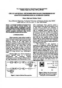
The first set of conducted experiments has been associated with a collection of pictures called Simulated Martian Rocks. The pictures were prepared by the Advanced Concepts Team and contained consistently illuminated stones arranged in a way that they create a complete background (see figure 1b). Occasionally, a white model of a spacecraft was inserted in the stones (see figure 1a), and such pictures constituted oddballs. The collection contained in total 3204 different background and 25 oddball images. Such a set of pictures complies directly with the classical oddball paradigm (Hruby and Marsalek (2002)). The picture collection has been used in several experiments whose aims were the following: • confirm that the P300 signal can be reliably detected with our experimental set-up and available tools, i.e., to a certain extent replicate the results obtained by Hruby and Marsalek (2002) (Experiment 1, Calibration); • analyse how the reliability of the detection of the P300 signal is affected by the rate of the image presentation (Experiment 2, Presentation Rate);
13
(a)
(b)
Figure 1: Examples of an oddball (a) and non-oddball (b) images from the Simulated Martian Rocks collection. • investigate if P300 activity is also evoked when the image presentation rate rules out conscious perception of visual stimuli (Experiment 3, Subconscious Perception); • assess the impact of potential memorisation of the presented image sequence after several repetitions by the subject on the detection of the P300 (Experiment 4, Learning). Every experiment involved presentation of one or more image sequences to the subjects. Before the start of the experiments, the subjects were verbally instructed to count images containing the spacecraft model and were presented examples of an oddball and non-oddball image. After that, the actual sequence of the images was presented while biometric measurements were being taken, always preceded by a 5 seconds long countdown screen that allowed the subjects to prepare for the experiment, reducing the surprise effect on the start of the image presentation. In the following paragraphs detailed parameters of the four experiments are presented. Experiment 1, Calibration . As stated earlier, the goal of this experiment was to verify that the assumed experimental setup allows reliable P300 detection. Parameters of the experiment are shown in table 1 and explained below. The experiment involved 4 subjects and 5 different sequences of images. Each of these sequences consisted of 40 images, 4 of which were oddball images. Oddballs were placed randomly in the image sequence. The experiment was repeated twice (using the same 5 sequences) for each subject after an arbitrary rest period. Every image was presented to the subject for 500 milliseconds (Image Display Period, IDP), after which a neutral background appeared for another 500 milliseconds (Inter Image Period, IIP), resulting in one image per second presentation rate. Thus, the presentation of one complete image sequence in this experiment took 40 seconds. The relatively low image presentation rate in this experiment should allow very reliable detection of the P300 signal. 14
No. of subjects 4
No. of sequences 5
Images in seq. 40
Oddballs in seq. 4
Repetitions 2
IDP/IIP (ms) 500/500
T (s) 40
Table 1: Parameters of the Calibration experiment No. of subjects 4 4 4 4 4
No. of sequences 5 5 5 5 5
Images in seq. 40 67 133 200 400
Oddballs in seq. 4 7 13 20 40
Repetitions 2 2 2 2 2
IDP/IIP (ms) 500/500 300/300 150/150 100/100 50/50
T (s) 40 40 40 40 40
Table 2: Parameters of the Presentation Rate experiment Experiment 2, Presentation Rate . As the goal here was to understand how fast the images can be presented to the subjects while still registering a P300 response, this experiment involved image sequences of different lengths presented with increasing image presentation rate. The number of images was adjusted to the change in presentation rate, so that the total duration of one sequence remained equal to 40 seconds. The number of oddball images present in the sequence was adjusted accordingly, so that the ratio of the number of oddball images to the number of non-oddball images was kept to the same level (10%). The oddballs were placed randomly in the sequences. As for the first part of the experiment, since all parameters are identical to the ones used in the Calibration experiment, the results of the latter were re-used. Parameters of the experiment are presented in Table 2. Experiment 3, Subconscious Perception . In order to check if the brain activity related to oddballs can be detected even when the image presentation rate is too high to allow conscious perception, a much higher image presentation rate than in the first two experiments has been used here and no inter-image blank was used (IIP=0). Two timing options have been used, resulting in displaying 30 and 60 images per second respectively, which is higher than the commonly agreed threshold of conscious perception, being 20 images per second (Hoshiyama et al. (2003)). For these two options, 10 different image sequences have been used, each of them containing exactly one oddball image (this fact however was not known to the subject). The oddball image placement was random, however it was enforced that it is placed within the first third of the sequence for 3 out of 10 sequences, within the middle third for 4 out of 10 sequences and within the last third for the remaining 3 sequences. All parameters of this experiment are summarised in table 3. Experiment 4, Learning . Finally, the issue of learning the image sequence by the subject in the case of a subsequent presentation of the same image sequence, and 15
No. of subjects 4 4
No. of sequences 10 10
Images in seq. 300 600
Oddballs in seq. 1 1
Repetitions 2 2
IDP/IIP (ms) 33.3/0 16.7/0
T (s) 10 10
Table 3: Parameters of the Subconscious Perception experiment No. of subjects 4
No. of sequences 5
Images in seq. 100
Oddballs in seq. 10
Repetitions 5
IDP/IIP (ms) 100/100
T (s) 20
Table 4: Parameters of the Learning experiment its impact on the P300 detection was addressed. In this experiment, a slightly different protocol than in the previous ones was used. Each of the subjects was shown 5 different image sequences, but each one of them was repeated 5 times one time after another. Moreover, the subject was made aware of this fact in advance, being verbally instructed that “the same image sequence is going to be repeated 5 times”. Relatively high image presentation rates have been used in order to evoke mistakes on behalf of the subjects and to allow the observation of a learning effect, if present. All parameters of the experiment are given in Table 4. 3.4.2
Collection 2: Optimization Visualizations
[ESA] The second set of conducted experiments aimed to answer questions concerning the relation between ERPs and expert knowledge and scientific curiosity. In order to meet these objectives, a special set of visual stimuli has been used, as well as two types of experimental subjects—a person with profound scientific knowledge about the stimuli (expert) and non-experts. The visual stimuli used in this second set of experiments were taken from ESA’s database of “multilayer coatings for thermal applications” 4 . The database contains images obtained during the process of designing a multi-layered material exhibiting predefined thermal emissivity profiles (which are called targets). Spectral directional properties of a material can be presented as 2-dimensional contour plots with axes representing angle and wavelength parameters and with the colour of the point representing the magnitude of the target parameter (for example emittance). Different materials, including the ideal target solution, correspond to different plots which appear as different 2-dimensional contours. However, as a material matching exactly the desired properties is not obtainable, the best found solution will only be similar to a certain degree to the ideal target solution. This “degree of similarity” is related to a simple pattern matching process (e.g. the image looks similar to the target image) in non-expert subjects, and to more complex cognitive processes in the expert (e.g., consideration on the physics of the 4
The database can be visited at the link www.esa.int/gsp/ACT/nan/op/bigrunresults.htm
16
(a)
(b)
(c)
(d)
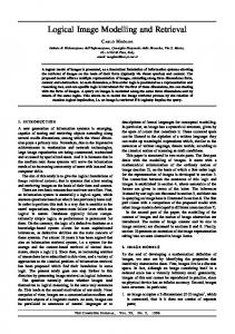
Figure 2: Examples of a target (a), obvious oddball (b), non-obvious oddball (c) and background (d) images used in the first experiment of the second phase.
17
No. of subjects
No. of targets
4+1
2
No. of sequences per target 5
h
Images in seq.
Oddballs in seq.
Repetitions
IDP/IIP (ms)
T (s)
50
3+3
2
500/0
25
Table 5: Parameters of the Expertise experiment emissivity profiles, experience of what can be considered a good match for the emissivity pattern, etc.). The image sets used were taken from different optimisation experiments for different desired ideal properties of the material and for solutions of different quality. The contours were plotted in a normalised range of parameter values and stripped from the axes and the legend. This image set was used to conduct experiments aimed to answer the following questions: • Is there a difference in P300 responses between subjects who possess scientific knowledge about presented stimuli and non-expert subjects? (Experiment 5, Expertise) • Is a subject’s scientific curiosity imprinted on the brain wave activity?(Experiment 6, Curiosity) Experiment 5, Expertise . This experiment was designed to find out if there is a difference in P300 responses between subjects who possess scientific knowledge about presented stimuli and non-expert subjects. The experiment used a modification of the oddball paradigm, with two types of oddballs: obvious and non-obvious. In each session, the non expert subject was presented an image corresponding to the target solution and instructed to “look for similar images”. The subject was also shown an example image considered an obvious oddball in order to be informed about the amount of acceptable differences between target solution and “good” solutions. Then a sequence of images was presented, which contained plots of materials with properties different from the ideal target (background images), very similar to the target (obvious oddballs) and slightly similar to the target (nonobvious oddballs). Examples of such images are shown in Figure 3.4.2, whilst the parameters of the experiment are presented in Table 5. In total 5 subjects were used, 1 expert (the European Space Agency’s scientist conducting the aforementioned study on multi-layered materials) and 4 non-experts. Two different target images were used, with 5 image sequences prepared for each of them. Every sequence contained 3 obvious and 3 non-obvious oddballs. As in previous experiments, every measurement was conducted twice. A moderately fast image presentation rate without the Inter-Image Period was used, which resulted in sequences of 25 seconds in length. Experiment 6, Curiosity . This experiment was conducted on the expert subject only. No target image has been used. Non-interesting background images were 18
No. of subjects 1
No. of sequences 5
Images in seq. 50
h Oddballs in seq. 10
Repetitions 2
IDP/IIP (ms) 750/0
T (s) 37.5
Table 6: Parameters of the Curiosity experiment mixed with potentially interesting oddball images selected by researchers preparing the image sequences, and which represented material properties that may evoke a subject’s curiosity. The subject was instructed to “look for interesting properties in the displayed images”. Parameters of the experiment are shown in Table 6. Differently from the Expertise experiment, the (expert) subject is no longer asked to perform pattern matching. Instead, with this experiment we wish to assess the potentiality of a subject’s scientific curiosity being imprinted on his brain wave activity. Should we be able to subsequently train an artificial system that displays similar curiosity and attention properties to the ones of the scientist, that machine would be able to look for scientifically interesting features in images in the same way the scientist would. 3.4.3
Collection 3: SenseCam
To provide an analogue to the ESA expert experiments, we created the ‘SenseCam’ dataset, which is a collection of low-quality personal photographs taken by a SenseCam device (Smeaton et al., 2006). The SenseCam is a personal wearable camera, worn on the front of the body, suspended from around the neck with a lanyard. It is light and compact, about one quarter the weight of a mobile phone and less than half the size. It has a camera with a fisheye lens and a range of sensors for monitoring the environment by detecting movement, temperature, light intensity, and the possible presence of other people in front of the device via body heat. The SenseCam regularly takes pictures of whatever is happening in front of the wearer throughout the day, triggered by appropriate sensor readings. Images are stored on-board the device, with an average of almost 3,000 images captured in a typical day, along with associated sensor readings. As such, the images produced by the SenseCam are by their very nature, uniquely tied to the wearer of the SenseCam, as they capture the personal experiences of that subject in their everyday lives. Therefore, we hypothesized that if we were to examine the ERP responses of the owner of a SenseCam viewing their images, versus another subject viewing the same images, that different ERP’s should be elicited as the images should ‘mean’ something different to the owner of the images. Therefore we view this collection as being comparable to the optimization visualization collection, where we have effectively an ‘expert’ subject, the owner of the SenseCam’s images, and a set of non-expert subjects. Experiment 7, Directed Oddball . This experiment is designed to compliment experiment 5, where effectively we have an oddball detection task, and our subjects 19
h
No. of subjects 4+1
No. of sequences 1
Images in seq. 500
Oddballs in seq. 50
Repetitions 1
IDP/IIP (ms) 300/300
T (s) 300
Table 7: Parameters of the SenseCam directed task, Experiment 7
h
No. of subjects 4+1
No. of sequences 1
Images in seq. 500
Repetitions 1
IDP/IIP (ms) 300/300
T (s) 300
Table 8: Parameters of the SenseCam non-directed task, Experiment 8 are divided into an expert subject and non-expert subjects. The instructions for this experiment were that the oddball for detection were images of ‘people eating’. This topic was chosen as it was considered generic enough that both expert and non-expert should be able to distinguish if an image contains a view of someone eating. We consider this experiment to be a directed task, as the subjects are informed of what is the oddball. The parameters for this experiment are presented in Table 7. Experiment 8, Non-Directed Oddball . Like experiment 7, experiment 8 is designed to compliment experiment 6 in the optimization visualization experiment. In this experiment, no oddball definition is given at all. The instructions for the subject were simply to view a stream of images which were presented to them. The intention of this experiment was to determine if there were differences between what the expert subject found of interest, compared against what a non-expert subject found of interest. The experimental parameters for this activity are defined in Table 8 This concludes the current section, in which we have defined our experimental conditions including the apparatus, the datasets and the experimental parameters. The next section will provide a high-level overview of ERP’s, and our objectives in their study within the Curiosity Cloning project. The intention of the following section is to provide some context for our analysis of ERP’s such that the interpretation of results is more meaningful.
4
Event Related Potential (ERP)
Event Related Potentials (ERP) are ‘time locked’ responses of electrical activity in the brain which occur at approximately the same time after a given event or stimulus (Luck, 2005). Whilst individually observed events will have variance with the exact time and strength of brain activity, by taking a large sample of these we are able to construct averages which demonstrate the existence of an ERP in response to stimulus. The act of averaging multiple time locked readings should make a signal observable over the 20
background activity measured by the EEG. Therefore, if we have multiple readings of brain activity, taken at specific times after certain events, we have a set of data which can be utilized, either to average so as to demonstrate a particular ERP occurring, or alternatively to use the multiple individual sample to create models which can be used to classify a given time locked ERP response. The taking of multiple samples to construct an average sample is known as producing a ‘grand average’. Therefore, there are three fundamental objectives of these series of experiments detailed within this technical report; 1. The elicitation of ERP’s generated by a subject in response to varying experimental stimulus, 2. The averaging of these time locked ERP’s so as to observe the existence of a definitive signal which demonstrates the existence of an ERP in response to experimental conditions, and where possible, 3. The creation of a model(s) which trained with captured ERP data, are able to conduct discriminative classification, such that the model is able to distinguish ERP’s related to stimulus events from non-stimulus events. As a grounding in the context of our experiments, the ERP averaging technique is a long standing method used to distinguish EEG activity modulated by the internal processing of a stimulus or preparation of action for a subject. Due to the fact that these measured EEG signals are subject to the noise of other independent ongoing neural processes along with external environmental noise, multiple time locked averages are often used to elicit a visual representation of EEG activity related to a particular condition (i.e. the presentation of stimulus vs non-stimulus). In this report we will demonstrate that it is possible to both visibly and analytically differentiate and identify EEG activity for different visual stimuli in particular experimental constructs, utilizing our 4-node setup. Primarily we focus on differentiating EEG activity in response to the presentation of particular target images vs non-targets images where targets are present in varying probabilities in the image sequences. These images are labelled as interesting vs non-interesting (stimulus vs non-stimulus). The recording of a subject’s EEG data was taken from multiple sites on the subjects scalp, namely sites Pz,Cz,P3,P4, where these site locations are defined according to the international 10-20 system. The selection of these sites is centred around the area of the brain which is most likely to present a P300 ERP. The selection of these sites was based upon domain-expert advice, where our objective was to capture as much data from a P300 event, given that there would be some variability in the placement of nodes on the subjects scalp. During our experimentation, each of these sites showed a differentiated response at multiple time points in the signal (after averaging) which strongly indicated that the presentation of a target image (oddball stimuli), does indeed cause a detectable change in ongoing EEG activity detected across all channels. Examples given within this report show this activity for site Pz unless otherwise stated. 21
Figure 3: Subject Response, Oddball experiment, IDP 1000ms, IIP 0ms, Broken line is stimulus response
22
The first graph shown, Figure 3, is of a subjects Pz site for an oddball elicitation style experiment (with 10% target likelihood), where IDP is 1000ms and IIP is 0ms, and the data utilized is from the simulated Martian rocks. This graph is computed from 2701 time windows and band-passed at 0.1-60hz. The heavier black line represents the EEG activity associated with a non-stimulus presentation (grand average computed from 2364 trials), whilst the broken line represents the stimulus image response, contains spacecraft, computed from 337 trials. The difference in the number of trials is due to an oddball probability of 10%, therefore for any given experimental window, we can expect to have approximately ten times the non-stimulus data to average from, as opposed to stimulus data. This imbalanced data set will present challenges later in our classifier creation work. The key point to be noted from Figure 3 is that the EEG signal for stimulus versus non stimulus is tightly correlated up to a time of approximately 220ms, after which the averaged stimulus signal deviates from the non-stimulus signal. The stimulus signal has a negative component peak at approximately 375ms, followed by a positive component peak at 500ms, which fits with the research literature of the approximate behaviour of the P300. Further visible differentiated EEG activity continues up to 1100ms for this subject, which indicates that the size of the temporal window to utilize for classification requires careful consideration, as components of a stimulus waveform are presenting well after 500ms. The discussion of the presentation of a stimulus versus non-stimulus response here is important, because it is from these observations that we created our signal processing framework and analysis techniques. Nevertheless, this grand average demonstrates that indeed there is a clear difference between this subject’s response to a stimulus versus non-stimulus event. This graph demonstrates a meeting of our first and second objectives of this experiment, the elicitation and averaging of time-locked ERP’s in response to experimental stimulus. For certain classes of experimentation, these two objectives will be all we will be able to meet, whilst for other experiments we will have enough data in which to create classifiers for identification of these waveforms. The labelling of these components and the subsequent interpretation will be described and noted where viable, however due to a wide variety of factors including individual differences, such as age, time of day, task habituation and error or variation in node placement, a solid interpretation as to the underlying nature of these components can not be fully derived within the scope of these experiments. Specifically this can be seen as a limitation of the 4-node setup, that whilst with the 4-node setup we are able to differentiate signals in response to different experimental stimulus, we lack the spatial resolution in order to accurately determine the constituent ERP’s which comprise that signal. Literature is available discussing and evaluating factors from human vision to internal cognitive processes modulating the timing, spatial origins and subsequent amplitude of these visible features (Branston et al., 2005). That is within our experimental evidence, we can conduct classification and grand averages to demonstrate differences in waveforms generated from experimental conditions, but we are unable to accurately infer for each
23
of the ERP components which make up the waveform, what each represents, where in the brain they originated and what implications this may have in interpretation of the observed waveform. As a prerequisite to the interpretation of these graphs it should be kept in mind that peaks and components are not the same thing. There is nothing special about the point at which the voltage reaches a local maximum or minimum. This is because the measured voltages are the summation of a number of underlying spatially configured ERP components which cannot be separated due to the inverse problem, further exacerbated by the spatial resolution provided by our four node setup. There’s an infinite number of component configurations which can give rise to any visible signal (Luck, 2005). It is for this reason that the ERP analysis in this document serves to verify the existence and location of key time regions of the EEG channel signals where target stimulus dependent differences can be observed so as to confine the regions from where attributes(features) will be extracted to compose machine learning schemes able to differentiate and identify these signals as to whether they are target or non target images.
5
Signal Processing, Feature Extraction and Machine Learning
Put simply, the measurement of EEG data is the reading of electrical activity at multiple spatial locations on the scalp. The ability to take these readings and convert them into a form in which we can infer the likely presence of ERP’s in response to some experimental condition. To achieve this we require three key components, signal processing of the raw signal, feature extraction and machine learning algorithms executed to successfully classify events. Significant challenges exist however in the application of signal processing and machine learning techniques to the classification of raw EEG data from low spatial resolution setups such as the one considered here. Two fundamental problems are at the origin of noise in the signal produced by the simple EEG. Firstly an analogue-digital conversion is required, which introduces noise into the signal, commonly referred to as the ’Sensory Gap’ (Smeulders et al., 2000). Further, environmental factors such as strong electrical currents or fluorescent lighting can lead to interference in the signal and quality degradation. Specific environmental conditions were therefore carefully implemented to minimize these impacts, as described in earlier sections. Secondly, the variance in the subjects themselves is a significant factor which can impact upon both signal processing and subsequent construction of classifiers. This subject variance can include factors such as the placement of the nodes on the scalp or the subjects level of fatigue. Many techniques were investigated for feature extraction from the raw EEG data across available channels. These approaches yielded different results over different data sets, and many were subject specific and prone to over-fitting. A more generalised type of classification regime was needed which could be applied to any of the data sets in order to achieve a classifier of decent accuracy. The approach was required to utilize 24
both time and frequency data at differing degrees of resolution in the time-frequency domain. For each channel, the following features are extracted (the temporal offset of extraction is the presentation time of the stimulus to the subject): • 14 samples are extracted from the signal for the time-window between 220ms and 810ms, low-band filtered at a cut-off frequency of 14Hz. A time resolution of 40ms (inferior to any IDP) is thus here obtained. It is intended to encode the main structural differences in time observed in figure. 3 between oddballs and non-oddballs. • Spectral information –as obtained from the Fast Fourier Transform (FFT)– of the raw signal (the DC component is previously removed) during the time-window ranging from 220ms to 620ms in which the P300 is expected. 5 features are extracted for frequencies from 1hz to 15hz at a spectral resolution of 3Hz, which attempt to point out differences in the high frequencies over a short time-frame. • Additional spectral information of the low frequencies between 1Hz and 5Hz for the whole signal (time window between 220ms and 1000ms). 5 attributes are chosen, which thus encode changes at a resolution of 1Hz. This methodology intends to take advantage of both variations in time and frequency, and that it targets the specific features where changes are expected, where this expectation was derived from our earlier ERP analysis as shown in the previous section. Two degrees of resolution are combined to improve the quality of the data. Our primary objective is the capture of P300 events, however despite its name, in practice P300 events do not always occur at 300ms, and that there is a great degree of variation in individual samples, such that a P300 peak may well reach its maximum amplitude at 450ms rather than at 300ms, as documented by Comerchero and Polich (1999). Our approach attempts to account for such variability through the choice of carefully selected time-windowing models. Additional signal processing algorithms were experimented with, namely Principle Component Analysis (PCA) and Haar Wavelet Coefficients. Yet these demonstrated no additional performance gain to classification accuracy when combined with the methodology outlined. Before classification, samples are normalized into the range [-1,1] using a linear transformation. Finally, for each stimulus (either oddball or non-oddball) 24 attributes are extracted from each dataset. Since the EEG setup consists of 4 channels, an overall feature vector of 96 features per stimulus is gathered. This defines a key difference between our 4-node setup, and more sophisticated EEG devices which contain a greater number of nodes. Because we have fewer nodes at our disposal to analyse, it means we can conduct a far more intensive mining of the raw signal and derive a greater degree of information from each signal, than we would if more nodes were available, as otherwise we would have far too much data in order to process. As it is, the resulting feature vector length of 96 features is too many for classification given the number of training samples we have available. In the following subsection we will detail this problem and our attempts to resolve it. 25
5.1
Classifier Construction
The classification task we are attempting is a binary classification task, where samples belong to one of two classes. We therefore selected a Support Vector Machine (SVM) with a Radial Basis Function (RBF) kernel (Vapnik, 1995) as our main classification technique, already shown in Lotte et al. (2007) to be suited to the task of classifying ERP signals. Our implementation makes use of both the WEKA toolkit (Whitten and Frank, 2005) and the LibSVM library (Chang and Lin, 2001). Two fundamental machine learning challenges are encountered, namely that of the class imbalance problem, and the curse of dimensionality (Akbani et al., 2004). The first manifests itself in the probability of an oddball image, which is initially set to only 10%, meaning that we have far more non-stimulus sample on which to train than stimulus events. If we naively utilized all training samples, we would produce a very biased classifier, which would detected very few stimulus events, as they have such a low probability of occurring in the experimental data, yet it is precisely these events which we wish to capture. The second challenge is the curse of dimensionality, which results from the relationship between the number of oddball samples available for training and the length of the feature vectors. As specified in several of the experimental protocols, the duration of each trial is to remain constant (i.e. 40s), which therefore means that as the presentation speed is varied, then the number of oddballs presented will also vary. This meant that for the simulated Martian rocks experiments that large variations in the number of oddballs in each trial was presented, ranging from only 30 in the slowest case, and up to 382 for the fastest. This problem is highlighted in Table 9. Whilst this motivation for a fixed time trial length enabled a degree of cross-comparability between subjects and experimental parameters, it produced unforeseen challenges for the task of classifier creation. To address this issue, we pruned the feature vectors from their original length of 96 attributes to 35 attributes via an SVM attribute evaluator (as implemented in the Weka toolkit). This process was conducted on a per-subject basis, primarily as a consequence of the significant variations existing between participants, such that a common set of 35 attributes did not exist between all subjects and necessitated a per-subject approach. We arrived at the figure of 35 attributes through empirical testing, for which little performance degradation was recorded against longer feature vectors. Further pruning IDP / IIP 500ms 300ms 150ms 100ms 50ms
# Non-Oddballs (NO) 400 670 1330 2000 4000
# Oddballs (O) 30 61 164 230 382
Ratio NO/O 13.3 11 8.1 8.6 10.4
Table 9: Distribution of Oddball and Non-Oddball Stimulus in Experiments 1-2
26
did however lead to a pronounced drop-off in performance. Note that although this capacity to discard nearly two-thirds of our feature vector implies the presence of highly redundant or non-discriminative attributes, an automated methodology would turn out to be inadequate under the current conditions because of the strong fluctuations across subjects. An in-depth analysis was also performed to quantify the influence of each single channel during the classification procedure, in an attempt to assess whether all four channels provide meaningful information and should therefore be maintained, or whether on the contrary some of them should be discarded. The 35 most relevant attributes (as reported by the SVM attribute selection algorithm) were iteratively selected among all considered features for each dataset, and they were given a score according to their contribution. A score of 35 was given to the most relevant attribute and 1 to the least. Scores were then added up for each channel and compared, hence giving an insight into their individual impact on the overall classification. For all experiments and subjects, it was observed that two channels (Pz and P3, with 27% and 28% impact respectively) had consistently more effect on the overall classification than Cz and P4. Yet it was shown that all four channels do add relevant information, later employed by the classifier, and should thus be maintained for our recognition purposes. As for the class-imbalance problem, we implemented a modified bagging approach, similar to that of Natsev et al. (2005) where a balanced training set was constructed by considering on the one hand, a set of oddball samples, and on the other, an equal number of randomly-sampled non-oddballs. Note that this differs from traditional bagging approaches as only one of the classes is randomly sampled, rather than both classes, as we did not have sufficient oddball samples. Stratified cross-validation was then performed to iteratively build the classifier, whereby we instituted an approximate 66/33 split between training and test samples based upon the number of oddballs. Training was undertaken on a balanced dataset as constructed by the modified bagging approach. Testing however was carried out on a set of samples which preserved the ratio between oddballs and non-oddballs, therefore maintaining the true distribution of oddball versus non-oddball stimulus events. Because the actual distribution of ‘oddball’ events was only approximately 10%, we believed it to be an unfair reflection of classifier accuracy if we were to test on a balanced test set. For each of our folds, we over-sampled the number of ‘non-Oddball’ samples to construct our test set. Therefore, our training sets were comprised of approximately 66% of the ‘oddball’ samples, with a random selection of an equal number of ‘non-Oddball’ samples to create a balanced training set, but our test sets which utilized the remaining 33% of ‘oddball’ samples maintained a 10% ratio of Oddball to Non-Oddball distribution. Table 10 details the number of training and test samples used in each case. The crossvalidation methodology was constructed out of 30-folds, and for each fold a grid-search optimization was run to determine the best parameters (C,γ) for the SVM. Whilst this may be seen as over-fitting to a degree (indeed our test set could equally be regarded as a validation set because of the grid-search), the intention of these experiments is of
27
IDP / IIP 500ms 300ms 150ms 100ms 50ms
Training Set (O/NO) 20/20 40/40 100/100 160/160 300/300
Test Set (O/NO) 10/133 16/176 64/158 72/602 82/853
Table 10: Training and Test Set Distribution of Oddball (O) and Non-Oddball(NO) samples. a proof-of-concept nature so as to determine if classification is possible at all on this dataset, and if so, is it likely that decent performance can be reasonably obtained.
6
Experimental Results
In this section we will present the results from each of the prescribed experiments. Depending on the experiment, different evaluation methods will be used to present the results, as different experiments will lend themselves to differing forms of evaluation. Firstly we will briefly discuss the evaluation measures to be used within this section, then following on from this, we will present for each experiment the results.
6.1
Evaluation Methodology
A fundamental requirement of any scientific evaluation is evaluation. However, an important question is always what is being measured and why is it important? As such, we utilize three primary evaluation tools for evaluating the success of our work. The first of these has already been introduced, which is the grand average of the ERPs. This tool is important, as it demonstrates the successful detection of ERP’s in response to experimental stimuli, regardless of the accuracy of any constructed classifier. This approach highlights in a broad sense, what data can be successfully captured by the 4-node EEG setup. The second and third tools however are more traditional machine learning metrics, the Receiver Operating Characteristic (ROC) curve, and the Area Under Curve (AUC) measure. The ROC curve is a practical measurement device as it informs us the degree to which we can obtain capture the true-positive events (in our case the oddball events), and how many false-positives are required in order to attain that level. We regard it as a ‘practical’ measure, as a system creator can determine for themselves where the trade-off should be between capture of oddball events with little noise, but missing out on many oddballs, or the capture of a significant number of oddballs but at the expense of a greater number of false positives. When interpreting the ROC curve, the ideal point is at co-ordinates [0,1], the top-left corner. If a straight diagonal is drawn from points [0,0] through [1,1], it will represent a classifier which has produced a random ordering. Therefore when comparing ROC curves we can use these two extremes, the diagonal line 28
and the [0,1] co-ordinate, to determine how well a classifier performed between a random classification, and a perfect classification. The AUC measure provides a single figure of performance for a classifier. The AUC measure is the probability that given a random positive example, and random negative example, that the classifier will rank the positive example before the negative example.
6.2
Experiment 2
N.B. we jump straight to the presentation of the results from Experiment 2, reliability versus speed, as the first trial in this experiment corresponds to the Experiment 1 parameters. The reliability vs speed experiments served to determine up to what image presentation rates a difference in the EEG signals could be detected for the target vs non-target images. Firstly we present in Figure 4 the grand average ERP’s across all speeds for experiment 2.
Figure 4: Grand Averages, all speeds.
29
Subject 1 Subject 2 Subject 3 Subject 4 Average
500ms 0.8254 0.8297 0.9043 0.6946 0.8135
300ms 0.7997 0.8164 0.7844 0.8072 0.8019
150ms 0.7291 0.8012 0.6593 0.7948 0.7461
100ms 0.6702 0.7492 0.6282 0.7207 0.6821
50ms 0.6276 0.6114 0.6362 0.6524 0.6319
Table 11: AUC Values across subjects for Experiment 2. Averaged ROC curves 1 0.9
True Positives (TP)
0.8 0.7
IDP=IIP=500ms IDP=IIP=300ms IDP=IIP=150ms IDP=IIP=100ms IDP=IIP=50ms
0.6 0.5 0.4 0.3 0.2 0.1 0
0
0.2
0.4
0.6
0.8
1
False Positives (FP)
Figure 5: Averaged ROC Curves for Experiment 1. The arrow underlines the improvement, as measured by the AUC, as the speed is reduced.
As can be clearly seen from these averages, there is a distinct difference in the oddball versus non-oddball stimuli events, indicating that successful classification should be possible as the two stimuli present with different signals. We can see from these graphs a clear attenuation in both signals as the presentation time becomes quicker, which indicates that classification accuracy should similarly deteriorate as the presentation time increases. Nevertheless we are happy with the clear separation between the oddball and non-oddball stimulus which has been captured with the 4-node device. The next challenge is to determine if there is consistently enough of a difference between the two cases that an accurate classifier can be constructed. Presented in Table 11 is the AUC values per subject, and the overall averages, whilst Figure 5 presents the averaged ROC curves across each of the presentation times. The classification results of experiment 2 are very encouraging, with accurate classification achieved certainly in the case of the 500ms through to the 150ms experiments. 30
More surprisingly, given the limited nature of our 4-node hardware were the results of the 100ms and 50ms experiments, where a non-random classification was actually produced, inferring that the EEG device and our signal analysis was able to detect and extract stimuli responses at this very fast presentation speed. There are a few areas of note with these results. Firstly based upon the AUC values in Table 11, we can see that there is indeed significant variation between our subjects and the performance of classifiers built upon their data. This indicates that the subject themselves plays a significant role in the determination of classifier performance, particularly as we can see that for each of the speed experiments, different subject’s classifiers performed at different levels. That is, a subject from which a poor classifier was produced in the 500ms experiment, was actually a very good performer in the 300ms experiment. Secondly we would note that there is a minimal performance difference in both the averaged ROC curves and the average AUC values for the 500ms and 300ms experiments. We believe that a greater performance differential should have existed between these two approaches, and the reason that this does not exist is because of the lack of oddball stimulus event in the 500ms experiment (30 oddball events only). It may be the case that there is not as great a difference between these experiments because the subjects may have been less concentrated on the 500ms experiment, or as it was the first experiment they may have been adjusting to the task. Nevertheless it remains an open question for further investigation if performance gains can be attained with the 500ms experiment. The experimental data as it is, indicates there is little difference between 500ms and 300ms, therefore when designing our own experiments, that is why we chose 300ms as the presentation rate for the SenseCam experiments. The results from the reliability versus speed experiments exceeded our expectations of what was achievable with our 4-node setup, particularly in terms of what could be detected and exploited at the fast presentation speeds. We believe that the results demonstrated in this section highlight the viability of utilizing a cheap EEG device for oddball style experiments. Whilst it remains the case that this setup could not be utilized for the identification of specific ERP’s generated in response to stimuli, given the poor spatial resolution, it certainly provided enough data to capture two different signals which were produced by a subject in response to different experimental stimuli. Given therefore that the task here is that we only wish to identify for a particular visual stimulus if it elicits a different signal as compared to other visual stimuli, then the 4-node EEG setup would seem to be a viable device, particularly when coupled with our signal processing approaches.
6.3
Experiment 3 and Experiment 4
Unfortunately for experiments 3 and 4, there was insufficient data from which to base any firm conclusions about the outcomes of the experiments. Here we recall that experiment 3 was the ‘subconscious’ experiment, where very fast presentation rates of 33ms and 16.67ms was utilized. Unfortunately in these experiments, only one oddball was prescribed in the image sequence. This was insufficient from which to attempt to either 31
Figure 6: Subject Response, Subconscious at 33ms
produce a grand average, or construct a classifier. The main feedback from our subjects during this experiment was that of seeing an almost constant blur, akin to travelling at ‘warp speed’. This experiment could be revisited with a higher oddball presentation rate, however given the performance of the 50ms experiment previously discussed, we believe that the 33ms and 16.67ms experiments would not produce useful data when the 4-node device is employed. However, we can still examine the average signal produced by these experiments for the non-oddball stimuli. As can be seen in Figure 6 the heavy black line represents non stimulus presentation. Their is a clear elicitation of a SSVEP response at 60hz which can be seen visually in the raw signal view (sinusoidal shaped wave) along with a minor peak in the FFT transform at 60hz (averaged over 11981 samples). A discussion of SSVEP can be found at the end of this report. This confirms that there was the expected elicitation to the high visual presentation rate, however, there is not enough stimulus signals to average to reveal the elicited response to a target image (if there is one). Nevertheless, this graph demonstrates that the 4-node device was capable of capturing some readings from such a fast presentation speed. 32
Figure 7: Subject Response, Subconscious at 16.67ms
Similarly shown in Figure 7 for experiment 3.2 there is a SSVEP response at 30hz. These results as stated previously do not conclude that the target images failed to elicit a response, just that concrete conclusions cannot be made with such a low number of target stimulus time windows. Previous work has been conducted on a task similar to this and does provide evidence that this task might be possible (Bernat et al., 2001), however again we would highlight the difficulty we believe of our 4-node device in this task. Likewise, experiment 4 was designed to test habituation, that is the attenuation of an oddball response once a sequence is continually repeated, such that the subject knows when the oddball would occur. Like the previous experiment, we unfortunately lacked sufficient experimental data from which to draw conclusions from this experiment. Whilst the number of oddballs was higher than the previous experiment, the objective of this experiment was to examine attenuation between trials. Within an individual trial we lacked sufficient oddball examples from which to produce a robust grand average for each trial that could have been used for inter-trial comparison. Subject habituation however is a known factor in EEG studies, and has been previously studied. We are 33
confident that given a revised experimental design that a habituation response could be observed utilizing our 4-node setup.
6.4
Experiment 5
The results for experiment 5 signal the start of the more ambitious component of the Curiosity Cloning project, to attempt to see if we can capture differences between expert and non-expert subjects. The dataset for the next two experiments was the Optimization Visualizations data, and the subjects included one expert subject from the ESA, and four non-experts from DCU. This task became more ambitious as we moved from a binary class situation, of ‘oddball’ and ‘non-oddball’, to a tertiary class situation where we introduced the ‘non-obvious oddball’, a class of oddball that should be recognizable to the expert subject and should elicit an oddball response, where this response should be based upon more than just a subconscious ‘odd one out’ as the non-obvious oddball should require some deeper understanding of the displayed data. In Figure 8 the grand averages for each subject’s response to an oddball, non-obvious oddball, and non-oddball are presented, and Subject 6 is the expert subject. Similar to our previous experiments where grand averages were produced, for all subjects the grand average signal of the oddball classes is clearly distinguishable from the non-oddball class. This was encouraging as it demonstrated that the oddball paradigm was working with this new dataset which incorporate colour information. From this data we can see that several of the subjects do produce a notable difference in their signal response to oddball versus non-obvious oddball stimulus. In particular these are subjects 3, 4 and the expert subject 6, where the two oddball responses demonstrate a deviation from each other, and from the non-oddball response. As we have highlighted earlier, the spatial resolution of our 4-node EEG device is insufficient for identifying component ERP’s present within an observed signal. Therefore when examining this data, we cannot be certain as to what is actually causing this difference, if it is a different response in the amplitude of a P300 ERP, or if other ERP’s are presenting for these subjects upon recognition of the non-obvious oddball. However as we have previously discussed, for the purposes of what we are trying to achieve here in the construction of a classifier that can exploit this data, it is immaterial to us a systems builders which ERP’s are causing this differentiation. What is important is that a differentiation exists and can be detected, meaning that we should be able to construct classifiers which can distinguish between this type of data. We would note that we are not saying that the identification of the component ERP’s is not an important activity, rather that it is not required for this specific experiment. Therefore, the next step within this experiment is to attempt to construct classifiers which leverage this observed data. We will create two classes of classifier. The first will be a standard oddball/non-oddball classifier, similar to which was used in our previous experiments. For the creation of this classifier, the obvious oddballs and non-obvious oddballs are aggregated into a single oddball class. We do this, so as to determine what our approximate classifier accuracy is on a standard oddball task when utilizing this new dataset, where the construction of this classifier is in line with our previous methodology. 34
activation (ADC)
2180
2160
2160
2140
2140
2120
2120
activation (ADC)
300
400
500
600
700
2100 obvious oddball 200 800
non−oddball
2180
2160
2160
2140
2140
2120
2120
300
400
500
600
700
2100 200
800
Subject #5
2200
2180
2160
2160
2140
2140
2120
2120
2100 200
300
400
500 (ms)
600
300
700
2100 200
800
500
600
700
800
400
500
600
700
800
700
800
Subject #6
2200
2180
400
Subject #4
2200
2180
2100 200
300
non−obvious oddball
Subject #3
2200
Subject #2
2200
2180
2100 200
activation (ADC)
Subject #1
2200
300
400
500 (ms)
600
Figure 8: Averaged results for the three classes experiment, where Subject 6 is the expert.
35
subject 1 2 3 4 5 6
oddball vs. non-oddball AUC 0.80 0.84 0.78 0.85 0.81 0.68
obvious vs. non-obvious AUC 0.50 0.55 0.64 0.61 0.44 0.63
Table 12: AUC results for the second experiment The second classifier will be to determine if we can distinguish between the two oddball classes. It will remain a binary classifier, except that it will only operate on oddball data, attempting to classify between oddball and non-obvious oddball as the two classes. It attempts to recognize patterns that respond to a higher-level cognitive process related to scientific interest, even for images that are non salient, i.e. not clearly defined in terms of what constitutes an interesting one. We believe this approach has merit, because in a deployment scenario these two classifiers could be employed in conjunction, where the results of the first classifier (oddball versus non-oddball) feed into the second classifier so as to determine a finer granularity as to the type of oddball observed. The creation of the second classifier differs slightly from our earlier classification strategies. The training set consisted of 45 obvious target examples (randomly chosen) labelled as positive vs 45 non-obvious target example labelled as negative. Evaluation was carried out on a test set consisting of 32 mutually exclusive samples from the dataset (15 obvious and 15 non-obvious). This process was repeated 100 times to reveal the previous average ROC graph, and to produce an average AUC figure for obvious vs non-obvious classification. The results for both classifiers are presented in Table 12. The accuracy of classification in the ‘oddball’ vs. ‘non-oddball’ case is similar to the range of AUC values recorded in experiment 2, with AUC values around 0.80 for most subjects. The recognition between any oddball and non-oddball is thus not significantly affected by the current experimental conditions, which may therefore be used as a testbed to perform further studies beyond the oddball paradigm. An overall evaluation of our second analysis already points out that the recognition between obvious and non-obvious oddballs is somewhat more delicate. The performance is clearly degraded as compared against the general oddball classification, however an examination of the grand average signals demonstrates that whilst this differentiation exists in some subjects, it is not overly pronounced, therefore a decrease in classification accuracy would be expected. Nevertheless though, for our previously identified subjects which produced differentiated grand averages for the two oddball classes (subjects 3, 4 and 6), we were able to produce classifiers which achieved greater than 0.6 AUC, indicating that the classifier constructed was able to determine to some extent, which oddball were considered to be different to other non-obvious oddballs by the subject. This was an exciting result, as it was far from certain that any classification accuracy 36
above random could have been achieved. Note that the perspective here adopted is mainly computational, and that it is not intended to help conclude that fundamental neurophysiological differences underlie the mechanisms that generate the ‘obvious’ and ‘non-obvious’ signals. Our classification is indeed performed regardless of whether the neural mechanism at their origin is actually different or not. Note for instance that, even though subjects #3,#4 and #6 present similar performance, in the case of the latter expert subject, the differentiation seems to be related to a positive peak after 300ms, whereas for the first ones it results from an important negative deflection at 250ms. In the framework of our study, such differences do not provide any further insight into the classification problem and are hence treated identically.
6.5
Experiment 6
Experiment 6 was intended to utilize the expert subject, and to present to this subject a stream of images, where there was no prior information given as to what constituted an oddball event. The intention was to allow the subject to view the images to determine what the subject found of interest when there was no directed task. Unfortunately we did not carefully review the experimental parameters for this experiment, and a presentation time was chosen which was different to that of the previous experiment. The intention had been to utilize the classifiers constructed in experiment 5 for the expert subject, and apply them to the data produced in experiment 6, such that the classifier would predict what the subject found of interest. However as the presentation times differed it was not possible to produce comparable feature vectors which could have been applied for classification.
6.6
Experiment’s 7 and 8
The final two experiments prescribed were the most ambitious of the project, those which utilized the SenseCam images. The task as originally defined was to examine the set of natural images, which could contain places, people, objects etc, and to look for oddball images, where the oddball was images of people eating. Unfortunately however, we found that the SenseCam images presented considerable challenges as it produced far more complicated neurological responses. For instance, an ERP component known as a N170 can present itself upon the viewing of a face (Hoshiyama et al., 2003). In an of itself this may not have been a significant challenge, however if the oddball task was to detect images of people eating, then you are guaranteed to observe a face. Other challenges which the dataset produced was large variance in the lighting of the images, the recognition of people in images and the identification of temporal components within the dataset (i.e. a subject may recognize an order to the images and adjust to that). The end result of this is that the data produced was incredibly noisy, with many ERP’s being generated which were not present in the synthetic data of the previous experiments.
37
We did produce classifiers based upon our recorded data, and they did achieve an AUC value of 0.6. However, whilst hinted at in the previous section, we have no idea what ERP’s are being used as discriminators for the identification of the oddballs. In this instance this is important, particularly because of the issues that the faces introduced. We have no way in this case of knowing if what was constructed was actually a face classifier, rather than a people eating classifier, which is purely down to the complexity of the images which were presented to our subjects. Whilst this result was disappointing, it provided an invaluable learning experience about operating with EEG’s and utilizing non-synthetic datasets. The lessons learned from this experiment will provide a valuable reference for our future endeavours with EEG experimentation.
7
General Observations and Issues Encountered
This section is a catch-all section where we will attempt to document various lessons which we learned during the completion of the Curiosity Cloning project, and to highlight areas of interest and directions for further research. We hope that this section will act as a store of the general experience we derived through this project.
7.1
Discussion on the presentation of the average time-locked stimulus waveform
One of the challenges of conducting a visual RSVP oddball style experiment, is the presentation of what is known as a Steady State Visually Evoked Potential (SSVEP), which are natural responses to a visual stimuli at specific frequencies. This presents a challenge, as it means after the presentation of a visual stimulus, there will be an occurrence of a SSVEP which can interfere with the measurement of the following stimulus. From our earlier graphs, such as Figure 3 (IDP=1000ms,IIP=0ms) an overlap can be seen from the elicited target stimulus EEG response into the time window of the next image presentation. The effects and consequences of this phenomenon become more evident as we begin to lower the IDP presentation times as can be seen in Figure 9. Shown in fig Figure 9 are the grand average ERP waveforms with presentation rates of IDP=50ms and IIP=50ms. Averaged EEG activity for the oddball is shown in a broken line while non-oddball activity is shown in the a solid line. For this faster image presentation rate a clear SSVEP response can be seen. SSVEP’s are elicited when an image is presented at a consistent rate between 3.5hz and 75hz. These images in our case for the simulated Martian rocks experiments are the mere change between the blank greyscreen frame and the rock stimuli (either target or non-target). Examining this signal in the frequency domain reveals two dominant frequency components. The 10hz and 20hz component reflect the image presentation rates, i.e. 10 images per second, and 20 changes per second from image to greyscreen with a harmonic contribution from the 10hz component. Resolving ERP components from these averages which show a SSVEP response is difficult due to the high number of overlapping components. For
38
Figure 9: Subject Response, Oddball experiment, IDP 50ms, IIP 50ms, Broken line is stimulus response
39
instance Luck remarks: Steady-state ERPs have a significant shortcoming, however, which is that they do not provide very precise temporal information. For example, if stimuli are presented every 150ms, the voltage measured at 130 ms after the onset of one stimulus consists of the sum of the response to the current stimulus at 130ms, the response to the previous stimulus at 280ms, the response to the stimulus before that at 430ms, and so on (Luck, 2005) However, as we have previously established we are not identifying specific ERP components, so this is not as problematic as first thought. For instance in this Figure, we can see a deviation in the signal for the stimulus case beginning at 380ms and continuing as far as 800ms post stimulus. The corresponding averaged FFT frequency view confirms this with the presence of increased low frequency signal components which visually match what we observe in the signal view. This phenomenon can be seen throughout most users ERP averages for the Reliability Vs Speed experiments (where IDP,IIP=50ms,100ms,150ms,300ms). SSVEP high frequency components (and harmonics) can also be observed for the subconscious experiments 3.1 & 3.2 at 30hz and 60hz matching the image presentation rates.
7.2
The development of datasets and classification
Machine learning methods for discriminative classification engage effectively in pattern matching. The algorithms themselves do not know any higher order semantics about the data that they are being trained on, rather they seek just to find whatever patterns present themselves which allow for the creation of decision boundaries. As such, it is very easier to construct a classifier which the builder believes is trained on one particular artefact, but is in fact operating on a completely different artefact of the data. We highlighted this problem in our discussion of the SenseCam experiments, where we did achieve a classification accuracy of AUC 0.6, however upon reflection, knowing that ERP’s are generated in response to faces, and the task was that of finding people eating, we had no certainty as to what the classifier was actually discriminating on. Likewise we found that even for the carefully constructed simulated Martian rocks experiment, that if not careful, additional artefacts could be introduced which would aid classification accuracy and give a false performance metric on accuracy based upon EEG readings. Specifically, we note that visual ERP components have been noted to be sensitive to brightness. One observation made utilizing the simulated Martian rocks data set was that the distribution of image luminance was different for the oddball versus non-oddball targets. Luminance was calculated as the sum of RGB values. The average luminance for the target images was 77,738,512 compared to 75,743,685 for non-oddballs. Both of these figures are similar, however the range of image luminance is greater for the non-oddball images. This is relevant because there’s an increased likelihood of a larger change in luminance on the presentation of an oddball target stimulus image since when generating image sequences images were chosen randomly from the distribution. 40
Training an SVM classifier on values computed from the difference in luminance between the current presented image and the last presented image reveals that an approximate 68% classification accuracy can be achieved purely due to this difference in the luminance distribution between the oddball target and non-oddball images. This has consequence because some of the earlier visual ERP components are known to be sensitive to changes in brightness in their amplitudes and latency (Luck, 2005). Naturally with this finding, we did not exploit this data to assist in the classification process. However, this highlights that even in a carefully constructed dataset, which the simulated Martian rocks were, that additional artefacts can present themselves which can inadvertently assist in classification accuracy, and lead to over-fitting.
7.3
Node Placement Locations, the P3a and P3b
The sites Pz, Cz, P3, P4 were those at which we recorded throughout our experiment, these positions are as indicated by the international eeg 10-20 system. We were advised that as we were conducting an oddball style experiment, to use these node sites as the P3 ERP is typically described as being strongly detected around the parietal regions of the brain. Placing a distribution of nodes in this area did capture differentiating activity for oddball versus non-oddball images. However, including the data captured from each of the four channels did not in all cases bring a high increase in classification accuracy over using less nodes, even though the ERP averages across the channels would make it appear as though much more differentiating data was being captured. Firstly, mention should be made that the P3 component is composed of two parts, the P3a and P3b. P3a potentials are typically recorded earlier and have frontal-central generators in the brain. Their elicitation is more generally induced by the presentation of truly unexpected stimuli (to dangerously simplify). The P3b potential on the other hand, is more closely tied to simpler discriminative tasks and is recorded more strongly at parietal-occipital sites (Polich and Comerchero, 2003). The implication of this therefore, is that an area for future research, whilst still constraining ourselves to the 4-node setup, is to place our nodes in a greater spatial configuration, such that we can attempt to more reliably capture and identify potentials such as the P3a.
8
Conclusions
This reported detailed the activities and collaboration between DCU and ACT in the Curiosity Cloning project. The novelty of the approach which DCU brought to this experiment was the use of a cheap, commodity EEG device, consisting of 4-nodes. The use of a 4-node device brought a different frame of reference to these experiments. Where traditional EEG devices consisted of many nodes, the restriction of having only 4 nodes available meant that the spatial resolution of the device was limited. Concentrating the node placements around the Pz site, the intention was to capture
41
as much data as possible which would be generated from ERP’s associated with oddball events, notably the P300 ERP. However, due to the aforementioned reduced spatial resolution, this device could not accurately identify all the ERP components that comprised any given signal after stimulus presentation. Nevertheless the intention of this project was such that the identification of any specific ERP’s was not a requirement, rather what was required was the accurate detection of different signals which corresponded to different experimental stimuli. In that respect we believe we have achieved good success as the use of the 4-node setup has allowed for the construction of discriminative classifiers, which offer good accuracy in an oddball detection task utilizing visual stimuli with a presentation rate of up to 150ms. Important lessons were learned in completing this project, particularly about what a 4-node device is suited for, and what pitfalls can be easily encountered. The major lesson was the care required in the creation of datasets for experimentation. This was particularly noticeable in our SenseCam experiments, where because the stimulus utilized generated many ERP’s, the limited spatial resolution of the device constrained our ability to conduct any accurate measurement of what was occurring with the subject’s signal. To revisit our overall aims in conducting this project, we aimed to: • To develop a methodology for use with the 4-Node EEG for its application to an RSVP oddball experiment. • The construction of discriminative classifiers on a per subject basis for the differentiation of oddball from non-oddball stimulus. • To determine in an RSVP oddball experiment, what is the effect of the image presentation speed on both EEG readings and classification accuracy. • The expansion of the discriminative classes to include a ‘non-obvious oddball’ class, so as to assist in the capture of expert knowledge versus non-expert knowledge. • To determine if a subject’s scientific expertise is able to be captured within the experimental paradigm, where the comparison will be to examine differences in results from scientific experts and non-experts? We believe that we have met these aims, and achieved results which at the beginning of this project we were unsure were achievable with a 4-node device, such as being able to distinguish between sub-classes of oddball events, as discussed in the results of experiment 5. With careful planning of the experimental framework, we have shown the applicability of utilizing a 4-node setup for creating classifiers for oddball style experiments. This work in and of itself can be very much considered as a proof of concept. We do not consider the results presented in this report to be the maximum of what could be achieved with our experimental apparatus. Indeed we view these results as a strong justification for further work which examines the applications of using cheap, accessible EEG devices to a variety of challenging research problems.
42
Acknowledgments The authors wish to acknowledge the European Space Agency’s Ariadna scheme (www.esa.int/gsp/ACT/ariadna/index.htm) for having initiated and supported this research. The authors from DCU additionally wish to acknowledge Science Foundation Ireland under grant 07/CE/I1147 for partial support of this work.
References (2009). Curiosity cloning image viewer project homepage. Akbani, R., Kwek, S., and Japkowicz, N. (2004). Applying Support Vector Machines to Imbalanced Datasets. In Proceedings of the 15th European Conference on Machine Learning (ECML 2004), pages 39–50, Pisa, Italy. Bernat, E., Shevrin, H., and Snodgrass, M. (2001). Subliminal visual oddball stimuli evoke a P300 component. Clinical neurophysiology, 112(1):159–171. Branston, N., El-Deredy, W., and McGlone, F. (2005). Changes in neural complexity of the EEG during a visual oddball task. Clinical Neurophysiology, 116(1):151–159. Castano, A., Fukunaga, A., Biesiadecki, J., Neakrase, L., Whelley, P., Greeley, R., Lemmon, M., Castano, R., and Chien, S. (2008). Automatic detection of dust devils and clouds on Mars. Machine Vision and Applications, 19(5):467–482. Chang, C. and Lin, C. (2001). LIBSVM: a library for support vector machines. Chien, S., Sherwood, R., Tran, D., Cichy, B., Rabideau, G., Castano, R., Davies, A., Mandl, D., Frye, S., Trout, B., Shulman, S., and Boyer, D. (2005a). Using autonomy flight software to improve science return on earth observing one. Journal of Aerospace Computing, Information, and Communication. Chien, S., Sherwood, R., Tran, D., Cichy, B., Rabideau, G., Castano, R., Davies, A., Mandl, D., Frye, S., Trout, B., Shulman, S., and Boyer, D. (2005b). Using autonomy flight software to improve science return on Earth Observing One. Journal of Aerospace Computing, Information, and Communication, 2(4):196–216. Comerchero, M. and Polich, J. (1999). P3a and p3b from typical auditory and visual stimuli. Clinical Neurophysiology, 110(1):24 – 30. Gerson, A., Parra, L., and Sajda, P. (2006). Cortically coupled computer vision for rapid image search. IEEE Transactions on neural systems and rehabilitation engineering, 14(2):174–179. Girimonte, D. and Izzo, D. (2007). Artificial Intelligence for Space Applications, pages 235–253. Springer, London.
43
Hoshiyama, M., Kakigi, R., Watanabe, S., Miki, K., and Takeshima, Y. (2003). Brain responses for the subconscious recognition of faces. Neuroscience research, 46(4):435– 442. Hruby, T. and Marsalek, P. (2002). Event-related potentials-the P3 wave. Acta Neurobiologiae Experimentalis, 63(1):55–63. Lotte, F., Congedo, M., Lecuyer, A., Lamarche, F., and Arnaldi, B. (2007). A review of classification algorithms for eeg-based brain–computer interfaces. Journal of Neural Engineering, 4(2):R1–R13. Luck, S. (2005). An introduction to the event-related potential technique. MIT Press Cambridge, MA. Natsev, A. P., Naphade, M. R., and Tesic, J. (2005). Learning the semantics of multimedia queries and concepts from a small number of examples. In Proceedings of the 13th annual ACM international conference on Multimedia (MULTIMEDIA ’05), pages 598–607, Singapore, Singapore. Polich, J. and Comerchero, M. (2003). P3a from visual stimuli: typicality, task, and topography. Brain Topography, 15(3):141–152. Ruci´ nski, M. (2008). Curiosity cloning image viewer user’s manual. Technical Report CCIVUM01, European Space Agency, the Advanced Concepts Team. Available on line at http://www.esa.int/act. Smeaton, A. F., O’Connor, N., Jones, G., Gaughan, G., Lee, H., and Gurrin., C. (2006). Sensecam visual diaries generating memories for life. In Poster presented at the Memories for Life Colloquium 2006, British Library Conference Centre. Smeulders, A., Worring, M., Santini, S., Gupta, A., and Jain, R. (2000). Content-based image retrieval at the end of the early years. IEEE Transactions on Pattern Analysis and Machine Intelligence, 22(12):1349–1380. Sutton, S., Braren, M., Zubin, J., and John, E. (1965). Evoked-potential correlates of stimulus uncertainty. Science, 150(3700):1187. Vapnik, V. N. (1995). The nature of statistical learning theory. Springer-Verlag New York, Inc., New York, NY, USA. Whitten, I. H. and Frank, E. (2005). Data Mining: Practical Machine Learning Tools and Techniques; (2nd ed.). Morgan Kaufmann Publishers, San Francisco, CA, USA.
44