Abstract--A finite element method using curvilinear elements is presented for modeling the sliding surface in rotating electric machines. The advantage of the ...
Curvilinear Finite Elements for Modeling the Sliding Surface in Rotating Electrical Machines And Its Applications W. N. Fu, Zheng Zhang*, P. Zhou, D. Lin, S. Stanton and Z. J. Cendes Ansoft Corporation, Pittsburgh, PA 15219, USA *Whirlpool Corporation, Benton Harbor, MI 49022, USA In permanent magnet (PM) motors, cogging torque is one of the main causes of vibration and noise. The accuracy of the computation of the cogging torque is very sensitive to the quality of the mesh and the geometry of the airgap. The proposed FEM is applied to calculate the cogging torque of a permanent magnet motor. Different methods to reduce the cogging torque are evaluated and compared.
Abstract--A finite element method using curvilinear elements is presented for modeling the sliding surface in rotating electric machines. The advantage of the proposed method is that the mesh has the same curved shape as the geometry and thus numerical accuracy is improved when connecting the stator mesh and the rotor mesh across a sliding surface. The procedure is applied to the compution of cogging torque for a permanent magnet motor. Different methods to reduce the cogging torque are then evaluated and compared.
II. MESH CONNECTION
Index Terms--Cogging torque, curvilinear element, electric machine, finite element, permanent magnet.
The airgap of the motor is divided into two parts. One belongs to the stator mesh and another belongs to the rotor mesh. The stator mesh and the rotor mesh are generated independently. When the rotor rotates, the rotor mesh will rotate. The shape of the mesh is kept fixed. Assuming the nodes on the sliding surface on the rotor mesh are slave nodes, as shown in Fig. 1, one has:
I. INTRODUCTION The finite element method (FEM) for magnetic field computation is widely used to simulate the operation of electric machines [1]. In two dimensions, triangular finite elements with straight edges are most commonly used. To improve the accuracy of the field approximation, the magnetic vector potential can be expressed in terms of second-order shape functions. In these elements, the value of the magnetic potential at any point in the element is interpolated according to the values at six nodes. An obvious advantage of straight-sided elements is algebraic computation of the finite element integrals; its shortcoming is the loss of accuracy in modeling curved shapes. In electric machines, objects with circular shapes are very common. Thus the accuracy of the second-order elements is often lost due to poor geometric approximation. In electric machines, electromagnetic modeling must be able to account for mechanical displacement caused by the relative movement between the stator and the rotor. One simple and effective method to accomplish this is to separate the solution domain into a stationary part and a moving part [2]. The magnetic field formulation of each part is established in its own coordinate system without relative movement. The solutions of the two parts are connected together by using matching boundary conditions on the interface between the stator mesh and the rotor mesh. We will call this interface the sliding surface since the rotor mesh slides over the stator mesh along this interface. During rotation, the two surfaces on the two sides of the sliding surface may be inconsistent as the rotor rotates to a different position. To solve this problem and to increase the accuracy approaching the curved geometry, a curvilinear element is presented in this paper.
0-7803-8987-5/05/$20.00 ©2005 IEEE.
A9 = N1 A1 + N 2 A2 + N 3 A3 A10 = N 3 A3 + N 4 A4 + N 5 A5
where N is the shape function of the edge.
Stator mesh A1
A2 A9
A3
A4 A1 0
A5
Sliding surface Rotor mesh
A6
A7
A8
Fig. 1. A straight line sliding surface
With rotation machines, the sliding surface is a circle. At the initial position, the mesh on the two sides of the sliding surface can be consistent as illustrated in Fig. 2. However, after the rotor rotates, because the edge of the element is a straight line, the inner surface of the stator mesh and the outside surface of the rotor mesh on the two sides of the sliding surface may be inconsistent as illustrated in Fig. 3. In some areas there may be a gap between meshes; in other areas the mesh may overlap. Several methods can be used to solve this problem, such as shifting the nodes, modifying the mesh, or re-meshing the airgap. Here we employ curvilinear elements on the two sides of the sliding surface.
628
while the shape functions corresponding to each node are: N 0 = ζ 0 (2ζ 0 − 1) ⎫ ⎪ N1 = 4ζ 0ζ 1 ⎪ N 2 = 4ζ 0ζ 2 ⎪⎪ ⎬ N 3 = ζ 1 (2ζ 1 − 1) ⎪ ⎪ N 4 = 4ζ 1ζ 2 ⎪ N 5 = ζ 2 (2ζ 2 − 1) ⎭⎪
Stator mesh Sliding surface Rotor mesh Fig. 2. Stator mesh and rotor mesh at initial position
where
Mesh gap
ζ 0 + ζ1 + ζ 2 = 1
Mesh overlap
5
5
x = ∑ N k ( x, y )x k
y = ∑ N k ( x, y ) y k
k =0
III. FEM USING CURVILINEAR ELEMENTS A 2-D FEM is used to compute the magnetic fields in the cross-section (x-y plane) of electric machines. The magnetic vector potential has only the component in z direction. For simplicity, circuit coupling [3] is not addressed here.
5
A = ∑ N k ( x, y )Ak
3
ζ 0 ζ 1 ζ 02 ζ 0ζ 1 ζ 12 ]
1
5
(1)
0
2
1
4
ζ0
x
0
5
Original curved element in global coordinat es
2
0
P arent element in local coordinat es
Fig. 4. Isoparametric second-order curvilinear element
C. Space Discretization By applying Galerkin’s method and using the shape function N as the weighting function, the magnetic field equation becomes:
∫∫Ω (∇ × A)
T
(2)
⋅ ν∇ × NdΩ + ∫∫ σ Ω
∂A ⋅ NdΩ ∂t
= ∫∫ J ⋅ NdΩ + ∫∫ (∇ × H c ) ⋅ NdΩ Ω
Ω
(9)
The (x, y) global coordinates are transformed to the (ζ0, ζ1) local coordinates. The integration is done in local coordinates. Because the curvilinear element becomes a triangle in the local coordinates, the integration is still easy. Breaking the integrals into summations over the elements on the local coordinates yields:
(3)
Using the isoparametric second-order curvilinear elements in Fig. 4, the polynomial basis of the shape functions is [5]:
[1
3
4
B. Shape Functions In 2-D, the shape function N has components only in the z direction:
N = Nkˆ
ζ1
y
where A is the magnetic vector potential; ν is the reluctivity of material and σ is the conductivity. The first term on the right in (1) only exists in stranded windings where J is the winding current density; The second term on the right in (1) only exists in permanent magnets and ν equals to the equivalent reluctivity in the permanent magnet; Hc is the permanent magnet coercivity. In 2-D problems, supposing the solution domain is on x-y plane, A has only a z-directed component:
A = Akˆ
(8)
k =0
A. Field Equations Maxwell’s equations applied to airgap, iron core, stranded windings and PM regions give rise to the following diffusion equation [4]: ∂A = J + ∇ × Hc ∂t
(7)
k =0
Six points are required to transform from global coordinates to local coordinates. This allows the edges of the elements to be curvilinear. The coordinates and the magnetic potential are modeled by the same shape function. The magnetic vector potential can be expressed as:
Sliding surface
Fig. 3. Stator mesh and rotor mesh after rotation
∇ × (ν∇ × A) + σ
(6)
Therefore, the natural coordinates x and y can be expressed as:
Stator mesh
Rotor mesh
(5)
(4)
629
∫∫Ω [(∇ × A)
T
ˆ
e
]
⎤ ⎡ ∂A ⋅ν∇ × N J dζ 0 dζ 1 + ∫∫ ˆ ⎢σ ⋅ N ⎥ J dζ 0 dζ 1 Ωe ⎦ ⎣ ∂t
= ∫∫ ˆ [J ⋅ N ] J dζ 0 dζ 1 + ∫∫ ˆ [(∇ × H c ) ⋅ N ] J dζ 0 dζ 1 Ωe
(10)
Ωe
With anisotropy materials, the coordinates are rotated first so that x and y axes align with the axes of the material. The magnetic reluctivity can be expressed as the tensor:
⎡ν x ν =⎢
0⎤ ⎥ ⎣ 0 νy⎦
(11)
Fig. 5. A simple example to show the accuracy improvement
The Jacobian matrix of the coordinate transformation is: ⎡ ∂x ⎢ ∂ξ J =⎢ 0 ⎢ ∂x ⎢⎣ ∂ξ1
⎡4ξ − 1 4ξ 1 =⎢ 0 4ξ 0 ⎣ 0
∂y ⎤ ∂ξ 0 ⎥ ⎥ ∂y ⎥ ∂ξ1 ⎥⎦ 4(ζ 2 − ζ 0 ) − 4ξ 0
0
− 4ξ 1
4ξ 1 − 1 4(ξ 2 − ξ1 )
⎡ x0 ⎢x ⎢ 1 1 − 4ζ 2 ⎤ ⎢ x 2 ⎢ 1 − 4ζ 2 ⎥⎦ ⎢ x 3 ⎢x4 ⎢ ⎣⎢ x 5
y0 ⎤ y1 ⎥⎥ y2 ⎥ ⎥ y3 ⎥ y4 ⎥ ⎥ y 5 ⎦⎥
(12)
Fig. 6. Mesh in the airgap of the simple example
In straight-sided elements, the coefficients of the Jacobian matrix are constant, but in curvilinear elements their values change with position. Because the integrated function changes with position in the element, it is difficult to perform algebraic integration. Here Gauss-Legendre numerical integration [6] is used to evaluate the coefficients of the curvilinear element. D. An Example to Show the Accuracy Improvement The curvilinear element has been applied to model rotating 2-D transient FEM problems. The elements on the two sides of the sliding surface are curvilinear. The simple example in Fig. 5 having two permanent magnets and a coil is used to study the error in the computation. The rotor is made of iron. To enlarge the numerical error for comparison, a coarse mesh with about 1500 triangles in the airgap is used as shown in Fig. 6. When the rotor rotates, the coil should theoretically have no induced electromagnetic force. But because of numerical error, the computed electromagnetic force in the coil is not exactly equal to zero. The computed electromagnetic forces using the straight-sided element and the curvilinear element are shown in Fig. 7 and Fig. 8, respectively. In both cases the mesh density is the same. It can be seen that the accuracy is significantly improved with the new method.
Fig. 7. Induced e.m.f. using the straight-sided elements (emax = 0.0283 V)
Fig. 8. Induced e.m.f. using curvilinear elements (emax = 0.00625 V)
630
IV. COGGING TORQUE COMPUTATION
100
The cogging torque of a PM motor with 56 poles and 42 slots is studied using the curvilinear FEM. Due to symmetric geometry and current sources, only a 1/14 of the problem region is required for the solution domain. The cross-section of its geometry is shown in Fig. 9. Although applying a fractional slot pitch can significantly reduce the cogging torque, it will produce an unbalanced radius force [7] and will not be discussed here.
80 60 40
B-emf (V)
20 0 -10.0
-5.0
0.0
5.0
10.0
15.0
20.0
25.0
30.0
35.0
40.0
45.0
50.0
-20 -40 -60 -80 -100 Time (ms)
Fig. 11. Measured back e.m.f. of the motor at 149.5 rpm without load
B. The Basic Design The original design does not include any mechanism to reduce cogging torque. It uses straight permanent magnets along the axis. The surface of the stator teeth forms a circular arc which has the same center as the axis of rotation and has a uniform airgap. For calculating the cogging torque, the conductivities of all materials are set to zero. The rotor rotates at a constant speed of 1 degree/sec. Fig. 12 presents a plot of the cogging torque when the rotor rotates (360/42)×2=17.14 mechanical degrees, which is equal to the distance of two stator teeth. The magnitude of the cogging torque from the measurement is about 1.6 Nm and verifies the calculated results. A typical force density distribution is shown in Fig. 13. The no-load back e.m.f. is shown in Fig. 14. The load torque when the motor is at two-phase-on excitation with rectangular current waveform is shown at Fig. 15.
Fig. 9. The cross-section of the PM motor
A. Calculation of the back e.m.f. at no-load Comparing the calculated and measured back e.m.f. waveforms is an easy method to check whether the setup of the magnetic properties in the simulation is correct. In the experiment, another motor is required to drive the testing motor to a constant speed. The three windings of the testing motor are open-circuited. When the motor rotates at the speed of 149.5 rpm, the calculated and measured back e.m.f. waveforms are shown in Fig. 10 and Fig. 11, respectively.
Fig. 12. Computed cogging torque (|T|av=0.9847 Nm)
Fig. 10. Computed back e.m.f. of the motor at 149.5 rpm without load
631
Fig. 16. Computed cogging torque (|T|av=0.3159 Nm)
Fig. 13. Force density distribution
Fig. 17. Computed back e.m.f. (eef=84.19 V) at 300 rpm
Fig. 14. Computed back e.m.f. (eef=106.8 V) at 300 rpm
Fig. 18. Computed load torque (Tav=6.276 Nm) at 300 rpm
D. The Motor with Non-uniform Airgap Another method to reduce the cogging torque is to use a non-uniform airgap under the teeth. The surface of each tooth is still a circular arc but with a smaller radius. In this design, the minimum airgap is kept the same as in the original design. The shape of the teeth is shown in Fig. 19. The cogging torque, the no-load back e.m.f. and the load torque are shown in Figs. 20, 21 and 22, respectively.
Fig. 15. Computed load torque (Tav=8.014 Nm) at the speed of 300 rpm
C. The Motor with Large airgap A simple method to reduce cogging torque is to increase the airgap. The cogging torque, the no-load back e.m.f. and the load torque when the thickness of the airgap is doubled are shown in Figs. 16, 17 and 18, respectively.
632
Fig. 22. Computed load torque (Tav=7.213 Nm) at 300 rpm Fig. 19. A tooth with non-uniform airgap
E. The Motor with Skewed PM An effective method to reduce the cogging torque is to use skewed permanent magnets. For motors with skewed slots/permanent magnets, a multi-slice FEM model has been developed [8]. However, if only to calculate the cogging torque, the 2-D FEM model of each slice can be solved seperately. Here the model of the motor is seperated into 20 slices along the axial direction. The total torque is the average value of all slices. When the permanent magnets are skewed 0.26 of the tooth pitch with uniform airgap, the cogging torque, the no-load back e.m.f. and the load torque are shown in Figs. 23, 24 and 25, respectively. Fig. 20. Computed cogging torque (|T|av=0.2137 Nm)
Fig. 23. Computed cogging torque (|T|av=0.05603 Nm)
Fig. 21. Computed back e.m.f. (eef=96.71 V) at 300 rpm
633
V. CONCLUSION The proposed FEM using curvilinear element can significantly reduce the numerical error for connecting the stator mesh with the rotor mesh. It has been successfully applied to calculate the cogging torque of a PM motor. For the motor studied in this paper, the design using a nonuniform airgap under the teeth can significantly reduce the cogging torque. Skewed permanent magnets is the best way to reduce the cogging torque if manufacture process allows such structure.
Fig. 24. Computed back e.m.f. (eef=101.2 V) at 300 rpm
REFERENCES [1] [2] [3]
[4] [5] [6]
Fig. 25. Computed load torque (Tav=8.013 Nm) at 300 rpm
[7]
F. Comparison of the Design Methods The four designs are compared in Table I. It can be seen that the design using the skewed PM can significantly reduce the cogging torque, while keeping the back e.m.f. and the load torque almost the same as the basic design.
[8]
TABLE I COMPARISON OF DIFFERENT DESIGNS Basic Large-airgap Non-uniform Skewed-PM 0.3159 0.2137 0.05603 84.19 96.71 101.2 6.276 7.213 8.013
Cogging torque |T|av (Nm) 0.9847 Back e.m.f. eef (V) 106.8 8.014 Load torque |T|av (Nm)
634
P. Zhou, W.N. Fu, D. Lin, S. Stanton, Z.J. Cendes, “Numerical modeling of magnetic devices,” IEEE Trans. on Magn., Vol. 40, No. 4, July 2004, pp. 1803 - 1809. Rémy Perrin-Bit and Jean Louis Coulomb, “A Three Dimensional Finite Element Mesh Connection for Problems Involving Movement,” IEEE Trans. on Magn., Vol. 31, No. 3, May 1995, pp. 1920-1923. W.N. Fu, P. Zhou, D. Lin, S. Stanton, Z.J. Cendes, “Modeling of solid conductors in two-dimensional transient finiteelement analysis and its application to electric machines,” IEEE Trans. on Magn., Vol. 40, No. 2, March 2004, pp. 426-434. M.V.K. Chari and S.J. Salon, Numerical Methods in Electromagnetism, Academic Press, 2000. Nathan Ida and João P.A. Bastos, Electromagnetics and Calculation of Fields, Springer-Verlag New York, 1997. Jianming Jin, The Finite Element Method in Electromagnetics, John Wiley & Sons, 2002. W.N. Fu, Z.J. Liu, C. Bi, “A dynamic model of the disk drive spindle motor and its applications,” IEEE Trans. on Magn., Vol. 38, No. 2, March 2002, pp. 973-976. S.L. Ho, W.N. Fu, “A comprehensive approach to the solution of direct-coupled multislice model of skewed rotor induction motors using time-stepping eddy-current finite element method,” IEEE Trans. on Magn., Vol. 33, No. 3, May 1997, pp. 2265-2273.