Aug 13, 2010 - ABSTRACT. This work introduces personas, descriptions of fictional individuals used in the field of human-computer interac- tion, into the ...
Fourth National Conference of IBPSA-USA New York City, New York August 11 – 13, 2010
SimBuild 2010
CUSTOMIZING THE BEHAVIOR OF INTERACTING OCCUPANTS USING PERSONAS Rhys Goldstein, Alex Tessier, and Azam Khan Autodesk Research 210 King St. East, Toronto, Ontario, Canada, M5A 1J7 {firstname.lastname}@autodesk.com
ABSTRACT This work introduces personas, descriptions of fictional individuals used in the field of human-computer interaction, into the simulation of building performance. The ultimate goal is to reduce the impact of buildings on the environment by helping architects predict the energy demand associated with different design options. As energy consumption patterns are largely dependent on human activities, we previously developed a method to simulate the behavior of individual building occupants. Here we extend the method, allowing occupants to interact with one another. Also, whereas activities generated by the previous method were based on only the recorded schedules of real people, we now use personas as well to customize and diversify occupant behavior. Both occupant interaction and behavior customization were achieved via the assignment of weighting coefficients to activities used for model calibration. Simulation results demonstrate that, by supplying only modest amounts of information, architects may be able to generate plausible interdependent schedules specifically tailored to their own projects.
INTRODUCTION Buildings consume vast amounts of energy; they account for 72% of electricity use in the US, according to Crawley (2008). It has been suggested that appropriate design improvements, selected with the aid of decisionsupport software, could reduce energy use by about 30% in existing buildings and 50% to 75% in new buildings (Clarke 2001). This is the motivation for building performance simulation. The idea is to model a building’s many interacting subsystems, including its occupants, electrical equipment, and indoor and outdoor climate. With simulation results in hand, an architect is better able to predict the energy demand associated with various designs, and choose from among the more sustainable options. A building’s energy consumption patterns depend largely on the behavior of the people that occupy it, a fact observed in numerous papers comparing the timing of daily activities with profiles of energy use. Although many existing building performance simulation tools use fixed schedules to account for the presence of occupants, a study by Hoes et al. (2009) has shown that more detailed
occupancy models are necessary for accurate energy demand predictions. Having recently proposed a behavior simulation method for individual occupants (Goldstein, Tessier, and Khan 2010), we now turn our attention to the fact that buildings have multiple occupants, that those occupants interact with one another, and that the behavior of one occupant may differ from that of another. In pursuit of a multiple-occupant simulation method, we strive for both realism and ease of use. These qualities seem to conflict with one another, as the numerous input parameters required by realistic models can be difficult to obtain. For example, although our previous method generates realistic schedules that resemble the recorded schedules of real building occupants, architects would need to supply numerous schedules of their own to produce behavior specifically tailored to their own projects. This led us to a new idea: firstly, data extracted from recorded schedules could be packaged with simulation software and reused by many architects; secondly, descriptions of fictional individuals called personas could be invented by architects on a per-project basis to customize and diversify occupant behavior. Theoretically, the desired level of realism results from the large quantities of reusable recorded data, whereas the ease of use lies in the fact that each invented persona requires only a dozen or so parameters. The simulation method presented in this paper generates sets of schedules for arbitrary numbers of building occupants. The schedules feature occupant interaction. For instance, if an office meeting or social gathering appears in the schedule of one occupant, it will also appear in the schedules of other participating occupants. Also, the behavior represented in the schedules can be customized. Both occupant interaction and behavior customization are achieved with the same underlying mathematical technique: the assignment of weighting coefficients to the schedules and activities used for model calibration.
BACKGROUND An occupant schedule is a list of consecutive activities that describes the behavior of a building occupant over the course of a single day. An example of an occupant schedule is shown in Table 1. Each activity includes several activity attributes that pertain to a specific block of 252
Fourth National Conference of IBPSA-USA New York City, New York August 11 – 13, 2010
SimBuild 2010
time. In the example, these attributes include start times, tasks performed, numbers of participants, and durations inferred from consecutive start times.
Activity ID #0 #1 #2 #3 #4 #5 #6 #7 #8
Table 1: An occupant schedule Start Task Number of Time Performed Participants 00:00 off 1 10:13 work 1 12:37 break 3 13:24 work 1 14:31 break 1 14:36 work 2 14:49 break 2 15:02 work 1 15:48 off 1
Occupant behavior simulation is the process of generating fictional occupant schedules. We describe an occupant behavior simulation as schedule-calibrated if behavioral patterns found in the recorded schedules of real building occupants are automatically reproduced in the generated schedules. Notable work in schedule-calibrated simulation includes a presence/absence prediction model by Page (2007), a domestic occupancy model by Richardson, Thomson, and Infield (2008), and our own previous method described in Goldstein, Tessier, and Khan (2010). Each schedule-calibrated method involves a model calibration phase during which histograms are populated using the activities of recorded schedules. Providing a simple example, the histogram in Table 2 is populated with the data in Table 1. Observe that Activity #1, a transition from the off task to the work task occurring between 10:00 and 11:00, contributes a value of 1 to the off → work row and the column labeled 10. In practice, the time of day would be discretized at a higher resolution, and multiple schedules would contribute to the same histogram. Table 2: Histogram population Transition 10 11 12 13 14 off → off off → work 1 off → break work → off work → work work → break 1 2 break → off break → work 1 1 break → break
15
1
1
In Page’s method, the states present and absent are used in place of the tasks in Table 2, and hence there are four
possible transitions. Richardson, by contrast, tracks the number of active household occupants. If there are N occupants in total, then there are N + 1 states (0 to N active occupants) and (N + 1)2 possible transitions. Both Page and Richardson adopt a discrete-time approach in which exactly one transition occurs at every time step. Following this approach, one would have populated the work → work transition in column 11, condensed Activities #4, #5, and #6 into a single work → break transition, and treated the last two activities as a single break → off transition. As it is, the example reflects the discrete-event approach of our previous method, in which activity durations are tracked in separate histograms. We have yet to find a schedule-calibrated method in the literature with a convincing treatment of occupant interaction. If a five-person meeting is generated in the schedule of one occupant, for example, the same meeting should occur in the generated schedules of four other occupants. Our previous method produces numbers of participating occupants, but as in Page’s work, generated occupant schedules remain strictly independent. The problem with Richardson’s method is that, were it extended to include multiple tasks and applied to office buildings with dozens of occupants, the resulting number of possible transitions would render simulation intractable. Existing schedule-calibrated occupant behavior simulation methods also fail to provide easy-to-use mechanisms for customizing simulated behavior. Consider a scenario in which a client informs an architect that a future office building will accommodate different numbers of programmers, managers, marketers, and salespeople. Each type of occupant is expected to work different hours and favor different activities. One could model this diverse yet project-specific behavior by supplying their own schedules for calibration, but this would be prohibitively timeconsuming. In search of an easier way for architects to specify behavioral patterns on a per-project basis, we have been inspired by research in the field of human-computer interaction (HCI) on personas. A persona is a description of a fictional individual. In the HCI community, personas are invented by software designers who strive to better understand product requirements by imagining fictional characters as future users (Cooper 2004). A typical persona is assigned a portrait, a name like “Max” or “Jane Roberts”, and a 1-2 page description emphasizing personality traits and social/workrelated habits. Although personas usually emerge from observations and subjective decisions, Miaskiewicz, Sumner, and Kozar (2008) have proposed a method to identify them objectively by automatically classifying survey results. And while personas are generally qualitative in nature, they have been reduced to sets of quantitative attributes and analyzed numerically (Chapman et al. 2008). 253
Fourth National Conference of IBPSA-USA New York City, New York August 11 – 13, 2010
SimBuild 2010
OCCUPANT INTERACTION Here we extend our previous schedule-calibrated method to accommodate interaction between simulated occupants. Only one additional input parameter is required: the maximum number of building occupants N. Instead of generating each occupant schedule independently, we now generate N schedules simultaneously. During a simulation, a time variable t is repeatedly advanced to the end of the next activity to expire. When an occupant’s current activity expires, his/her subsequent activity is randomly generated from various probability distributions. These distributions depend on values extracted from the histograms populated in the calibration phase (see the Background section). As in Goldstein, Tessier, and Khan (2010), the generated activities have three attributes: the task, the duration, and the number of participating occupants n po . If n po = 1, the resulting solo activity has no effect on the schedules of other occupants. But if n po ≥ 2, then with our extended method, the resulting shared activity may appear in multiple occupant schedules. First, the initiating occupant (for whom the shared activity was generated) transitions to the new activity. Next, n po −1 summoned occupants are selected at random as additional participants. Note that the distinction between the initiating occupant and the summoned occupants is to be completely invisible to a simulation user. We introduce the distinction not as an attempt to model the real-world roles of group members, but only to produce interdependencies between the N generated schedules. Suppose that at time t we have just generated a shared activity, appended it to the schedule of the initiating occupant, and selected n po − 1 summoned occupants. Somehow the shared activity must be added to the summoned occupants’ schedules. We consider different options. The first option is to apply the shared activity immediately; that is, to prematurely terminate the current activities of all n po − 1 summoned occupants, and append the new shared activity to the n po − 1 associated schedules. Thus all n po occupants would begin the shared activity at time t. In the case of an office meeting, all attendees would arrive at exactly the same time. Some might leave early, however, to attend other meetings. A second option is to queue the shared activity. Each summoned occupant would transition to the shared activity only after the scheduled completion of his/her current activity. This option would allow participants to arrive late for a meeting, though all participants would leave the meeting at exactly the same time. To account for both planned and impromptu meetings, we decided on a compromise between the two options described above. First, bn po /2c of the n po − 1 summoned occupants are selected. These occupants abandon their current activities, and immediately switch to the shared
activity. The remaining summoned occupants complete their current activities, and thereafter transition to the shared activity. With this approach, some occupants may arrive late to a meeting, and some may leave early. So far we have described a simple extension to our previous schedule-calibrated method, facilitating occupant interaction by allowing shared activities to appear in multiple schedules. There is one important issue we must now address. First note that our previous method assumes every shared activity to be initiated by every participating occupant. The frequency with which simulated occupants initiate shared activities thus reflects the frequency with which real occupants interact. But now that an occupant can be summoned by other occupants, the frequency with which simulated occupants participate in shared activities will be overestimated. The problem is severe, as an n po person activity will occur roughly n po times too often. The solution to the above problem is to reduce the probability of initiating an n po -person activity by a factor of n po . This is done by assigning a weighting coefficient of 1/n po to each activity in the recorded schedules used for calibration. These coefficients affect the histogram population procedure discussed in the Background section. Table 3 shows the same histogram as in Table 2, again populated with the data in Table 1, but this time using weighting coefficients. For example, because Activity #2 (starting at 12:37) has 3 participating occupants, we now add 1/3 instead of 1 to the appropriate bin in column 12 of Table 3. Similar adjustments are made to the 2-person activities (Activity #5 at 14:36, and #6 at 14:49). Table 3: Histogram population with weighted activities Transition 10 11 12 13 14 15 off → off off → work 1 off → break work → off 1 work → work work → break 0.33 1.5 break → off break → work 1 0.5 1 break → break This application of weighting coefficients reduces the rate at which simulated occupants initiate shared activities, compensating for the fact that they may be summoned to activities initiated by others. Later in the paper we use different sets of non-negative weighting coefficients to influence behavior in other ways. Note that in Goldstein, Tessier, and Khan (2010), a recorded activity may contribute to multiple bins in each of several histograms. An activity’s weighting coefficient simply multiplies every value added to any bin in any histogram. 254
Fourth National Conference of IBPSA-USA New York City, New York August 11 – 13, 2010
SimBuild 2010
BEHAVIOR CUSTOMIZATION With existing schedule-calibrated methods, all of a building’s simulated occupants exhibit some sort of “average” behavior. There is no easy way to specify that certain occupants arrive unusually early, for example, or that others spend long hours in meetings. Here we introduce personas into building performance simulation as a way of customizing simulated behavior. In the HCI community, software designers invent personas to better understand the habits of users of future computer applications. In a similar way, we envision architects inventing personas to better predict occupant behavior in future buildings. Although HCI personas tend to be qualitative in nature, our focus on simulation necessitates hard numbers. Like Chapman et al. (2008), we regard a persona as a set of quantitative persona attributes. To describe an office worker, for example, useful persona attributes might include the arrival time, the percentage of the day spent in meetings, and the number of breaks taken each day. Chapman et al. caution that the more attributes a persona is given, the fewer real-world people it is likely to represent. We address this concern by expressing persona attributes as intervals. Instead of stating that an occupant arrives at 09:00, spends 5% of the day in meetings, and takes 3 breaks each day, we might state that he/she arrives between 08:45 and 09:15, spends 3% to 7% of the day in meetings, and takes 2 to 4 breaks. Each interval has an associated probability (eg. “...arrives between 08:45 and 09:15, 80% of the time). An architect who shares the concerns of Chapman et al. would choose large intervals. From an simulation user’s perspective, we feel that the intervals described above are relatively easy to interpret. However, from a mathematical perspective, it is more convenient to parameterize each persona attribute with a mean value µ and a standard deviation σ. If µ and σ are known, then the interval bounds blower and bupper associated with a probability of p may be calculated from (1). Similarly, if the interval is known, one may derive µ and σ from (2). We use Φinv to denote the inverse cumulative distribution function of a standard normal distribution. � � 1+ p ·σ blower = µ − Φinv 2 (1) � � 1+ p bupper = µ + Φinv ·σ 2 blower + bupper 2 bupper�− blower� σ= 1+ p 2·Φinv 2 µ=
(2)
We distinguish between two types of personas: inferred personas and invented personas. In the case of an inferred persona, m persona attributes are obtained from n
occupant schedules and their associated weighting coefficients. Recall that a weighting coefficient pertains to a single activity, and that there are several activities in an occupant schedule. We require a single weight for each schedule. Therefore, for each occupant schedule j (meaning the schedule identified by the integer j; j = 0, 1, . . . , n−1), we calculate the weight w j by averaging the weighting coefficients of the schedule’s activities. Continuing this persona inference procedure, the next step is to obtain a separate schedule attribute aij for each persona attribute i and occupant schedule j. The derivation of aij depends on the type of persona attribute. If the attribute quantifies an office worker’s arrival time, for example, we assign to aij the time between midnight and the first office activity of the day. If the persona attribute is the percentage of time spent in meetings, then aij is calculated by dividing the accumulated time spent in meetings by the time elapsed between arrival and departure. Once all n weights w j and all m·n schedule attributes aij are obtained, one can calculate the mean value µi and standard deviation σi for each persona attribute i. This is done by first evaluating nw using (3), then obtaining each µi and σi in that order using (4) and (5). n−1
nw =
∑ wj
(3)
1 n−1 · ∑ w j ·aij nw j=0
(4)
j=0
µi =
v u u 1 n−1 σi = t · ∑ w j ·(aij − µi )2 nw j=0
(5)
The inferred persona is completed by applying (1) for each persona attribute to obtain the corresponding interval. Slightly complicating matters, the probability p must in some cases be adjusted to yield a reasonable-sounding interval. Suppose, for example, that an arbitrarily selected p of 80% yielded an interval of -2 to 5 breaks per day. To avoid the negative number, we would instead report 0 to 3 breaks with a recalculated p of 42%. Inferring a persona from existing schedules, as described above, is a relatively simple procedure. Considerably more difficult is the use of an invented persona to generate fictional schedules. Note that we are not giving up on schedule-calibrated methods, for the inclusion of recorded schedules alleviates the need to obtain all behavioral information from user-supplied personas. However, in a case where recorded behavior contradicts an invented persona attribute, it is the attribute that should govern the behavior of the simulated occupant. A solution to this customization problem is to use our previous schedule-calibrated method, but steer the simulated behavior towards that of an invented persona using 255
Fourth National Conference of IBPSA-USA New York City, New York August 11 – 13, 2010
SimBuild 2010
a00 − µ0 σ0
2
···
a0 j − µ0 σ0
···
2
(a00 − µ0 ) −1 σ0 2 .. .
···
ai0 − µi σi
···
(ai0 − µi )2 −1 σi 2 .. . a(m−1)0 − µm−1 σm−1 �2 a(m−1)0 − µm−1 −1 σm−1 2
···
··· ···
(a0 j − µ0 ) −1 σ0 2 .. . aij − µi σi
···
···
(aij − µi )2 −1 σi 2 .. . a(m−1) j − µm−1 σm−1 �2 a(m−1) j − µm−1 −1 σm−1 2
···
0 .. .
···
0
···
··· ··· ···
0
rA
···
···
a0(n−1) − µ0 σ0 �2 a0(n−1) − µ0 −1 σ0 2 .. . ai(n−1) − µi σi �2 ai(n−1) − µi −1 σi 2 .. . a(m−1)(n−1) − µm−1 σm−1 �2 a(m−1)(n−1) − µm−1 −1 σm−1 2 0 .. . 0
rA ···
0
w0 . .. · w j .. . wn−1
=
rA
0 0 .. . 0 0 .. . 0 0 rA .. . rA .. . rA
Figure 1: The matrix equation A·W = B used to obtain weights from schedules and an invented persona weighting coefficients. Whereas persona inference entails the use of n schedules and n weights to calculate m persona attributes, we are now given m persona attributes and n schedules with which to obtain n weights. Assuming that the invented persona is specified using intervals, we first obtain the µi and σi of each persona attribute i using (2). We also calculate each schedule attribute aij as described above for persona inference. Now that the weights w j and their sum nw are unknown, it is best to eliminate nw from (4) and (5) by substitution using (3). Further manipulation yields (6) and (7).
tions for n unknowns. This motivates a least squares solution. Note that a large value of rA emphasizes (8). These n equations, which imply that w j = 1 for all j, steer the simulated behavior towards that found in the schedules. Conversely, small values of rA favor the persona. We have found that if there is a great discrepancy between the schedules and the invented persona, it is safest to use a large rA to discourage variability in the weights. We therefore recommend (9), which quantifies this discrepancy. Note that A2·m is the top 2·m-by-n submatrix of A, and B2·m is the top 2·m-element subvector of B. rA =k A2·m ·1n − B2·m k
n−1
aij − µi ·w j = 0 σi j=0 ! (aij − µi )2 − 1 ·w j = 0 σi 2
∑
n−1
∑
j=0
(6)
(7)
The obvious next step is to express (6) and (7) as a matrix equation of the form A·W = B. We do exactly that, as shown in Figure 1, but include (8) as well to avoid the trivial exact solution W = 0n (the vector W containing the unknown weights w j , and 0n being a vector of n zeros). rA ·w j = rA
(8)
With m equations given by (6), another m given by (7), and an additional n given by (8), we have 2·m + n equa-
(9)
The least squares solution is the W that minimizes k A·W −B k. Unfortunately, the standard solution neglects the fact that the weights must be non-negative. We recommend that W be obtained using the Fast Non-NegativityConstrained Least Squares Algorithm (FNNLS) of Bro and Jong (1997), which guarantees w j ≥ 0 for all j. Small values of r from (10) suggest a successful fit. r =k A2·m ·W − B2·m k
(10)
With W in hand, every activity of each schedule j can be assigned w j as a weighting coefficient. If the n schedules and the new weighting coefficients are used in the model calibration phase, the resulting simulated behavior should reflect both the schedules and the invented persona. 256
Fourth National Conference of IBPSA-USA New York City, New York August 11 – 13, 2010
SimBuild 2010
METHOD AND PROTOTYPE Occupant interaction and behavior customization can be combined into a single multiple-occupant simulation method. We tested this method by collecting behavioral data and implementing a prototype in C++. The method requires a set of recorded occupant schedules. For testing purposes, we gathered a total of 121 schedules from six researchers who tracked their own activities in an office environment. Each schedule resembled the example in Table 1, with possible tasks limited to off, desk work, desk meeting, team meeting, tech visit (eg. using the printer), washroom break, onsite break, and offsite break. Figure 2 shows the probability that an occupant is working at their desk (lower region) and engaging in shared activities with other occupants (upper region) throughout the day, based on these 121 schedules.
Figure 2: Activity profiles based on recorded schedules While recorded schedules can be packaged with simulation software and reused, the set of personas and the number of occupants for each persona are to be specified on a per-project basis. Our fictional building included 100 occupants and 3 personas: 50 occupants for Persona X, 40 for Persona Y, and 10 for Persona Z. Instead of inventing Persona X, we inferred its six persona attributes (m = 6) from the recorded schedules. Below, p = 50% for the desk meeting interval, and 80% elsewhere. Persona X (inferred from input data) ...arrives between 08:26 and 12:30 ...leaves between 15:29 and 21:44 ...spends 0.0% to 14.7% of the day in desk meetings ...has a 19.8% chance of meeting with the team ...takes a break onsite 0.2 to 3.2 times per day ...has a 51.2% chance of taking a break offsite For the persona attributes pertaining to team meetings and offsite breaks, the probabilities listed are the mean values µ. The intervals and standard deviations are redundant for these attributes, as σ = µ·(1 − µ). As for
the schedule attributes, aij = 1 if schedule j includes any team meeting/offsite break, and 0 otherwise. Both Persona Y and Persona Z were invented. Note the differences between the behavior specified below for Persona Z, and that inferred from the recorded schedules. Persona Z (invented) ...arrives between 10:00 and 11:00 ...leaves between 18:00 and 21:00 ...spends 10.0% to 20.0% of the day in desk meetings ...has a 40.0% chance of meeting with the team ...takes a break onsite 1.0 to 3.0 times per day ...has a 20.0% chance of taking a break offsite Before simulating interacting occupants, a set of nind independent schedules must be generated for each persona. We used nind = 10000, generating the Persona X schedules with our previous schedule-calibrated method. For each invented persona like Y and Z, one must first customize behavior by generating n independent schedules, constructing the matrices of Figure 1, and solving for W . We used n = 400. If there is a significant discrepancy between the n schedules and an invented persona, a single application of the FNNLS algorithm may be inadequate. Fortunately, the customization procedure can be repeated several times over. On each iteration, the current W is used to generate a new set of n schedules, which in turn yields an updated W . The value of r tends to decrease with each iteration, as each successive set of n schedules better reflects the persona. We terminate the loop when r ≤ 0.1, which required 3 iterations for both Persona Y and Persona Z. Final sets of weights are used to generate the sets of nind schedules. For each persona, one now has nind independent schedules with which to calibrate a separate activity generator. It is at this point that one applies the occupant interaction weighting scheme, where each n po -person activity is given a coefficient of 1/n po . When an occupant’s current activity expires during a simulation, the activity generator associated with his/her persona produces the next activity. The final challenge is to allow occupants of multiple personas to be summoned to the same shared activity, yet preserve the behavior in the independent schedules. Our solution is to use all sets of nind schedules to calibrate a single participant generator. Whenever an activity generator outputs a shared activity, the participant generator calculates the proportion of the summoned occupants to allocate to each persona. These proportions are selected in the same way that task probabilities were obtained in our previous method. All four activity attributes (time of day, task, n po , duration) are used as factors (see Goldstein, Tessier, and Khan (2010)), and there is one feature for each persona. A set of normalized feature values gives the distribution of personas among activity participants. 257
Fourth National Conference of IBPSA-USA New York City, New York August 11 – 13, 2010
SimBuild 2010
There is one remaining complication. If there are relatively few occupants of a particular persona, then those occupants will be summoned to a disproportionately high number of shared activities. Once again, an appropriate set of weighting coefficients solves the problem. Recall that the participant generator is calibrated with nind schedules of each persona. We weight each set of nind schedules with the overall fraction of occupants sharing the corresponding persona. In our prototype, for example, the coefficients for the three personas were 0.5, 0.4, and 0.1.
SIMULATION RESULTS We simulated the behavior of the 100 interacting occupants over a 24-hour period, 1000 times. The activity data accumulated from the 100,000 resulting schedules was used to create the profiles in Figure 3.
From a qualitative point of view, the results are as expected. The simulated Persona X profiles of Figure 3 resemble those of the recorded schedules in Figure 2. Persona Y was designed to exhibit an early schedule and relatively few shared activities, and this behavior is reflected in Figure 3. Similarly, the profiles for Persona Z are consistent with the invented attributes, exhibiting a later schedule and a greater prevalence of shared activities. We also inspected a sample of the generated schedules, looking at each activity. The schedules appeared plausible. To quantitatively validate the customization technique, personas were inferred from the 10000 (nind ) independent schedules. To validate the occupant interaction technique, we also inferred personas from the schedules of the interacting occupants. Shown below is the invented version of Persona Y, following by the two inferred versions. The desk meeting intervals have probabilities of 68% for the independent simulated occupants and 42% for the interacting occupants. For all other attributes, p = 80%. Persona Y (invented) ...arrives between 08:30 and 09:00 ...leaves between 17:00 and 18:00 ...spends 0.0% to 4.0% of the day in desk meetings ...has a 10.0% chance of meeting with the team ...takes a break onsite 0.0 to 2.0 times per day ...has a 60.0% chance of taking a break offsite Persona Y (independent simulated occupants) ...arrives between 08:29 and 09:00 ...leaves between 16:54 and 18:11 ...spends 0.0% to 3.8% of the day in desk meetings ...has a 12.3% chance of meeting with the team ...takes a break onsite 0.0 to 2.0 times per day ...has a 59.1% chance of taking a break offsite Persona Y (interacting simulated occupants) ...arrives between 08:30 and 09:00 ...leaves between 16:56 and 18:11 ...spends 0.0% to 4.9% of the day in desk meetings ...has a 14.3% chance of meeting with the team ...takes a break onsite 0.0 to 2.1 times per day ...has a 63.3% chance of taking a break offsite
Figure 3: Activity profiles based on the simulated behavior for Personas X (top), Y (middle) and Z (bottom)
Note the agreement between the invented version of Persona Y and the version inferred from the independently generated schedules. Although there are differences between the two sets of intervals, these differences pale by comparison to the discrepancy one would expect to observe between predicted and actual occupant behavior. As a similar level of agreement was achieved for Persona Z, we have confidence in the customization aspect of our method. 258
Fourth National Conference of IBPSA-USA New York City, New York August 11 – 13, 2010
SimBuild 2010
Similarities between the two inferred versions of Persona Y indicate that occupant interaction was introduced without severely altering behavioral patterns. It is worth noting, however, that the prevalence of shared activities is consistently higher in the version with occupant interaction. The most prominent discrepancy occurred in the team meeting attribute of Persona Z; with an invented probability of 40%, the independent schedules yielded 40.4%, but with interaction the result was 59.4%. For every other attribute, this bias was observable, but tolerable.
DISCUSSION Deserving mention is the USSU system developed by Tabak (2008), which implements its own occupant behavior simulation method. The method features both occupant interaction and behavior customization, and also includes spatial building information. Though USSU likely satisfies the need for realism, it appears to require numerous input parameters. The method is not schedulecalibrated, and without recorded schedules to inform simulated behavior, the simulation user must cope with a separate set of tasks for each type of occupant, several attributes per task, and various “task groups”. With our method, architects would benefit from recorded schedules provided with simulation software. If they opted to supply only a few persona attributes, or even none whatsoever, the software would still produce realistic behavior. We envision a workflow in which, at the beginning of a project, an architect would select only two parameters: the type of building (eg. office building, household, shopping mall) and the total number of occupants. The software would then skip the customization procedure, and produce realistic simulated behavior using the tasks and recorded schedules provided for the selected building type. Later, to account for differences between company workers, ages, genders, or cultural traits, personas would be added. This could be done gradually. As an architect designs floor plans and selects specific materials, his/her model might expand from zero personas, to a few personas with a few attributes each, to perhaps a dozen detailed personas. At a late stage in the design process, he/she may even include personas for occasional guests, or office workers who typically work from home.
CONCLUSION We have contributed a new method for simulating interacting building occupants exhibiting customized behavior. The behavior customization aspect of the method performed well, and should provide an easy way for architects to generate fictional occupant schedules specifically tailored to their own projects. Our treatment of occupant interaction is simple and viable, though further refinements may be needed to address its tendency to increase the prevalence of shared activities. In the future, we plan
to enhance the method with spatial information, and integrate it with models of electrical equipment and other energy-consuming building subsystems.
ACKNOWLEDGMENT We thank Michael Glueck, Ebenezer Hailemariam, and Xiaojun Bi for contributing many of the recorded schedules used to test the presented method.
REFERENCES Bro, Rasmus, and Sijmen De Jong. 1997. “A Fast NonNegativity-Constrained Least Squares Algorithm.” Journal of Chemometrics 11 (5): 393–401. Chapman, Christopher N., Edwin Love, Russell P. Milham, Paul ElRif, and James L. Alford. 2008. “Quantitative Evaluation of Personas as Information.” Proceedings of the Human Factors and Ergonomics Society 52nd Annual Meeting. New York, NY, USA. Clarke, Joe A. 2001. Energy Simulation in Building Design. second. Butterworth-Heinemann. Cooper, Alan. 2004. The Inmates are Running the Asylum. Sams Publishing. Crawley, Drury. 2008. “Building Performance Simulation: A Tool for Policymaking.” Ph.D. diss., University of Strathclyde, Scotland. Goldstein, Rhys, Alex Tessier, and Azam Khan. 2010. “Schedule-Calibrated Occupant Behavior Simulation.” Proceedings of the Symposium on Simulation for Architecture and Urban Design (SimAUD). Orlando, FL, USA. Hoes, Pieter-Jan, Jan Henson, M.G.L.C. Loomans, B. de Vries, and D. Bourgeois. 2009. “User behavior in whole building simulation.” Energy and Buildings 41 (3): 295–302. Miaskiewicz, Tomasz, Tamara Sumner, and Kenneth A. Kozar. 2008. “A Latent Semantic Analysis Methodology for the Identification and Creation of Personas.” Proceeding of the Conference on Human Factors in Computing Systems (SIGCHI). Florence, Italy, 1501–1510. Page, Jessen. 2007. “Simulating Occupant Presence and ´ Behaviour in Buildings.” Ph.D. diss., Ecole Polytechnique F´ed´erale de Lausanne, Switzerland. Richardson, Ian, Murray Thomson, and David Infield. 2008. “A high-resolution domestic building occupancy model for energy demand simulations.” Energy and Buildings 40 (8): 1560–1566. Tabak, Vincent. 2008. “User Simulation of Space Utilisation: System for Office Building Usage Simulation.” Ph.D. diss., Eindhoven University of Technology, Netherlands.
259