Aug 24, 2008 - Carnegie Mellon University. {leili,wenjief,fanguo ... are widely used in time series analysis such as motion capture mod- eling, visual tracking ...
Cut-And-Stitch: Efficient Parallel Learning of Linear Dynamical Systems on SMPs Lei Li, Wenjie Fu, Fan Guo, Todd C. Mowry, Christos Faloutsos Carnegie Mellon University
{leili,wenjief,fanguo,tcm,christos}@cs.cmu.edu
ABSTRACT
ables in both models are inferred through a forward-backward procedure involving dynamic programming. However, the maximum likelihood estimation of model parameters is difficult, requiring the well-known Expectation-Maximization (EM) method [1]. The EM algorithm for learning of LDS/HMM iterates between computing conditional expectations of hidden variables through the forwardbackward procedure (E-step) and updating model parameters to maximize its likelihood (M-step). Although EM algorithm generally produces good results, the EM iterations may take long to converge. Meanwhile, the computation time of E-step is linear in the length of the time series but cubic in the dimensionality of observations, which results in poor scaling on high dimensional data. For example, our experimental results show that on a 93dimensional dataset of length over 300, the EM algorithm would take over one second to compute each iteration and over ten minutes to converge on a high-end multi-core commercial computer. Such capacity may not be able to fit modern computation-intensive applications with large amounts of data or real-time constraints. While there are efforts to speed up the forward-backward procedure with moderate assumptions such as sparsity or existence of low-dimensional approximation, we will focus on taking advantage of the quickly developing parallel processing technologies to achieve dramatic speedup. Traditionally, the EM algorithm for LDS running on a multicore computer only takes up a single core with limited processing power, and the current state-of-the-art dynamic parallelization techniques such as speculative execution [6] have few benefits due to the nontrivial data dependencies. As the number of cores on a single chip keeps increasing, soon we may be able to build machines with even a thousand cores, e.g. an energy efficient, 80-core chip not much larger than the size of a finger nail was released by Intel researchers in early 2007 [10]. This paper is along the line to investigate the following question: how much speed up could we obtain for machine learning algorithms on multi-core? There are already several papers on distributed computation for data mining operations. For example, “cascade SVMs” were proposed to parallelize Support Vector Machines [9]. Other articles use Google’s mapreduce techniques [8] on multi-core machines to design efficient parallel learning algorithms for a set of standard machine learning algorithms/models such as naïve Bayes and PCA, achieving almost linear speedup [4, 12]. However, these methods do not apply to HMM or LDS directly. In essence, their techniques are similar to dot-product-like parallelism, by using divide-and-conquer on independent sub models; these do not work for models with complicated data dependencies such as HMM and LDS. 1
Multi-core processors with ever increasing number of cores per chip are becoming prevalent in modern parallel computing. Our goal is to make use of the multi-core as well as multi-processor architectures to speed up data mining algorithms. Specifically, we present a parallel algorithm for approximate learning of Linear Dynamical Systems (LDS), also known as Kalman Filters (KF). LDSs are widely used in time series analysis such as motion capture modeling, visual tracking etc. We propose Cut-And-Stitch (CAS), a novel method to handle the data dependencies from the chain structure of hidden variables in LDS, so as to parallelize the EM-based parameter learning algorithm. We implement the algorithm using OpenMP on both a supercomputer and a quad-core commercial desktop. The experimental results show that parallel algorithms using Cut-And-Stitch achieve comparable accuracy and almost linear speedups over the serial version. In addition, Cut-And-Stitch can be generalized to other models with similar linear structures such as Hidden Markov Models (HMM) and Switching Kalman Filters (SKF). Categories and Subject Descriptors: I.2.6 Artificial Intelligence: Learning - parameter learning D.1.3 Programming Techniques: Concurrent Programming - parallel programming G.3 Probability and Statistics: Time series analysis General Terms: Algorithms; Experimentation; Performance. Keywords: Linear Dynamical Systems; Kalman Filters; OpenMP; Expectation Maximization (EM); Optimization; Multi-core.
1.
INTRODUCTION
Time series appear in numerous applications, including motion capture [11], visual tracking, speech recognition, quantitative studies of financial markets, network intrusion detection, forecasting, etc. Mining and forecasting are popular operations we want to do. Two typical statistical models for such problems are hidden Markov models (HMM) and linear dynamical systems (LDS, also known as Kalman filters). Both assume linear transitions on hidden (i.e. ’latent’) variables which are considered discrete for the former and continuous for the latter. The hidden states or vari-
Permission to make digital or hard copies of all or part of this work for personal or classroom use is granted without fee provided that copies are not made or distributed for profit or commercial advantage and that copies bear this notice and the full citation on the first page. To copy otherwise, to republish, to post on servers or to redistribute to lists, requires prior specific permission and/or a fee. KDD’08, August 24–27, 2008, Las Vegas, Nevada, USA. Copyright 2008 ACM 978-1-60558-193-4/08/08 ...$5.00.
1
Or exactly, models with large diameters. The diameter of a model is the length of longest acyclic path in its graphical representation. For example, the diameter of the LDS in Figure 1 is N .
471
Symbol Y Z m H N F G
Definition a multi-dimensional observation sequence the hidden variables (= {z1 , . . . , zN }) the dimension of the observation sequence the dimension of hidden variables the duration of the observation the transition matrix, H × H the project matrix from hidden to observation, m × H
5
zn+1 yn
5;&ͼ
1
ɇ
G
1
z
,
)
1
z
,
ȿ
5;&ͼnj ȿ
͙
2
,
)
Z
5;'ͼ
2
2
z
,
ɇ
)
)
5;'ͼ
Z
3
ɇ
3
z
,
)
Z
5;'ͼ
N
�
N
�
,
5;&ͼ
1
ɇ
1
z
1
z
, N
�
ȿ
)
Z
N
5 'ͼ
ɇ
(
)
z
N
,
)
Y N
1
2 Y
3
�
1
Y
Y
N
Figure 1: A Graphical Representation of the Linear Dynamical System: z1 , . . . , zN indicate hidden variables; y1 , . . . , yN indicate observation. Arrows indicate Linear Gaussian conditional probabilistic distributions. Given the observation sequence, the goal of the learning algorithm is to compute the optimal parameter set θ = (µ0 , Γ, F, Λ, G, Σ). The optimum is obtained by maximizing the log-likelihood l(Y; θ) over the parameter set θ. As mentioned in Section 1, the typical learning method for LDS is the EM algorithm [1], which iteratively maximizes the expected complete log-likelihood in a coordinateascent manner: Q(θnew , θold ) = Eθold [log p(y1 . . . yN , z1 . . . zN |θnew )] In brief, the algorithm first guesses an initial set of model parameters θ0 . Then, at each iteration, it uses a forward-backward algorithm to compute expectations of the hidden variables ˆ zn = E[zn | Y; θ0 ] (n = 1, . . . , N) as well as the second moments and covariance terms, which is the E-step. In the M-step, it maximizes the expected complete log-likelihood of E[L(Y, z1...N )] with respect to the model parameters. Since the computation of E[zn | Y] depends on E[zn−1 | Y] and E[zn+1 | Y], the straightforward implementation of the EM algorithm can not exploit much instruction level parallelism. Although we will focus on LDS in the rest of this paper, our CutAnd-Stitch method could also be adapted to HMMs with a careful replacement of context, because their graphical models are very similar. Figure 1 shows the structure of the graphical representation of an LDS; notice that the structure remains the same for hidden Markov models, with the only differences that the hidden (and possibly observed) variables are discrete and that the conditional distributions should be replaced by multinomial distributions. Accordingly, the forward-backward algorithm of HMM is still tractable and can be implemented in a similar manner, and the M-step in the learning algorithm can be modified as well.
3. CUT-AND-STITCH: PROPOSED METHOD In the standard EM learning algorithm described in Section 2, the chain structure of the LDS enforces the data dependencies in both the forward computation from zn (e.g. E[zn | Y; θ]) to zn+1 and the backward computation from zn+1 to zn In this section, we will present ideas on overcoming such dependencies and describe the details of Cut-And-Stitch parallel learning algorithm.
3.1 Intuition and Preliminaries
(1) (2) (3)
Our guiding principle to reduce the data dependencies is to divide LDS into smaller, independent parts. Given a data sequence Y and k processors with shared memory, we could cut the sequence into k subsequences of equal sizes, and then assign one processor to each subsequence. Each processor will learn the parameters, say θ1 , . . . , θk , associated with its subsequence, using the basic, sequential EM algorithm. In order to obtain a consistent set of parameters for the whole sequence, we use a non-trivial method to
where z0 is the initial state of the whole system, and ω0 , ωi and ǫi (i = 1 . . . M) are multivariate Gaussian noises: ω0 ∼ N (0, Γ) ωi ∼ N (0, Λ)
)
Y
BACKGROUND
z0 + ω0 Fzn + ωn Gzn + ǫn
,
(
Here we give a brief introduction to Linear Dynamical Systems (LDS), including its formalization, its learning algorithm and its connections to hidden Markov models (HMM). Consider a multi-dimensional sequence Y = y1 , . . . , yN of a length N. For example, Y could be a sequence of marker position vectors captured by video cameras, where each vector yi is of dimensionality m. Suppose the evolution of the observation is driven by a hidden Markov process. For example, in motion capture modeling, hidden variables may correspond to a sinusoid moving pattern, while the observed motion could be periodic walking cycles. In LDS, both the transitions among the hidden variables as well as their projections to the observations are described as linear Gaussian models (Eq (2-2)). We denote them as a matrix F for the transition (H × H) with noises {ωn }; and a matrix G (m × H) for the projection with the noises {ǫn } at each time-tick n. Figure 1 provides the graphical representation of following equations defining an LDS: = = =
ȳ
0
5 ͼ
In this paper, we propose the Cut-And-Stitch method (CAS), which avoids the data-dependency problems. We show that CAS can quickly and accurately learn an LDS in parallel, as demonstrated on two popular architectures for high performance computing. The basic idea of our algorithm is to (a) Cut both the chain of hidden variables as well as the observed variables into smaller blocks, (b) perform intra-block computation, and (c) Stitch the local results together by summarizing sufficient statistics and updating model parameters and an additional set of block-specific parameters. The algorithm would iterate over 4 steps, where the most timeconsuming E-step in EM as well as the two newly introduced steps could be parallelized with little synchronization overhead. Furthermore, this approximation of global models by local sub-models sacrifices only a little accuracy, due to the chain structure of LDS (also HMM), as shown in our experiments, which was our first goal. On the other hand, it yields almost linear speedup, which was our second main goal. The rest of the paper is organized as follows. We first describe the Linear Dynamical System in Section 2 and present our proposed Cut-And-Stitch method in Section 3. Then we describe the programming interface and implementation issues in Section 4. We present experimental results Section 5, the related work in Section 6, and our conclusions in Section 7.
z1
u
Z
Table 1: Symbol table
2.
(
ǫj ∼ N (0, Σ)
472
ʐ Ɍ ɻ Ɏ 1
,
1
,
1
,
ʐ Ɍ ɻ Ɏ
1
2
,
2
,
2
,
2
.
.
all blocks on each processor, the block parameters should be well chosen with respect to the other blocks. We will describe the parameter estimation later but here we first describe the criteria. From the Markov properties of the LDS model, the marginal posterior of zi,j conditioned on Y is independent of any observed y outside the block Bi , as long as the block parameters satisfy:
.
͙
P (zi,1 |y1 , . . . , yi−1,T ) = P (zi+1,1 |y1 , . . . , yN ) = Figure 2: Graphical illustration of dividing LDS into blocks in the Cut step. Note Cut introduces additional parameters for each block.
P (zi,j |yi,1 . . . yi,j ) = P (zi,j |yi,1 . . . yi,T ) =
Pi,j−1 Ki,j µi,j Vi,j
(12)
= FVi,j−1 FT + Λ
(13)
= Pi,j−1 GT (GPi,j−1 GT + Σ)−1 = Fµi,j−1 + Ki,j (yi,j − GFµi,j−1 ) = (I − Ki,j )Pi,j−1
(14) (15) (16)
Ki,1 µi,1 Vi,1
= = =
Φi GT (GΦi GT + Σ)−1 υi + Ki,1 (yi,1 − Gυi ) (I − Ki,1 )Φi
(17) (18) (19)
The backward passing equations are: Ji,j µ ˆi,j ˆ Vi,j
= Vi,j FT (Pi,j )−1 = µi,j + Ji,j (ˆ µi,j+1 − Fµi,j ) ˆ i,j+1 − Pi,j )JTi,j = Vi,j + Ji,j (V
(20) (21) (22)
The initial values are given by: Ji,T µ ˆi,T ˆ Vi,T
(4) (5) (6) (7)
= Vi,T FT (FVi,T FT + Λ)−1 = µi,T + Ji,T (ηi − Fµi,T )
(23) (24)
= Vi,T + Ji,T (Ψi − FVi,T FT − Λ)JTi,T
(25)
Except for the last block: µ ˆk,T = µi,T
where the block size T = N and j = 1 . . . T indicating j-th varik ables in i-th block (zi,j = z(i−1)∗T +j and yi,j = y(i−1)∗T +j ). ηi , Ψi could be viewed as messages passed from next block, through the introduction of an extra hidden variable z′i,T . P (z′i,T ) = N (ηi , Ψi )
(11)
The initial values are given by:
The objective of Cut step is to compute the marginal posterior distribution of zn , conditioned on the observations y1 , . . . , yN given the current estimated parameter θ: P (zn |y1 , . . . , yN ; θ). Given the number of processors k and the observation sequence, we first divide the hidden Markov chain into k blocks: B1 ,. . . , Bk , with each block containing the hidden variables z, the observations y, and four extra parameters υ, Φ, η, Ψ. The sub-model for i-th block Bi is described as follows (see Figure 2): N (υi , Φi ) N (Fzi,j , Λ) N (Fzi,T , Λ) N (Gzi,j , Σ)
N (µi,j , Vi,j ) ˆ i,j ) N (ˆ µi,j , V
We can obtain the following forward-backward propagation equations from Eq (4-8) by substituting Eq (9-12) and expanding.
3.2 Cut step
= = = =
(9) (10)
Therefore, we could derive a local belief propagation algorithm to compute the marginal posterior P (zi,j |yi,1 . . . yi,T ; υi , Φi , ηi , Ψi , θ). Both computation for the forward passing and the backward passing can reside in one processor without interfering with other processors except possibly in the beginning. The local forward pass computes the posterior up to current time tick within one block P (zi,j |yi,1 . . . yi,j ), while the local backward pass calculates the whole posterior P (zi,j |yi,1 . . . yi,T ) (to save space, we omit the parameters). Using the properties of linear Gaussian conditional distribution and Markov properties (Chap.2 &8 in [1]), one can easily infer that both posteriors are Gaussian distributions, denoted as:
summarize all the sub-models rather than simply averaging. Since each subsequence is treated independently, our algorithm will obtain near k-fold speedup. The main design challenges are: (a) how to minimize the overhead in synchronization and summarization, and (b) how to retain the accuracy of the learning algorithm. Our Cut-And-Stitch method (or CAS) is targeting both challenges. Given a sequence of observed values Y with length of N, the learning goal is to best fit the parameters θ = (µ0 , Γ, F, Λ, G, Σ). The Cut-And-Stitch (CAS) algorithm consists of two alternating steps: the Cut step and the Stitch step. In the Cut step, the Markov chain of hidden variables and corresponding observations are divided into smaller blocks, and each processor performs the local computation for each block. More importantly, it computes the initial beliefs (marginal expectation of hidden variables) for its block, based on the neighboring blocks, and then it computes the improved beliefs for its block, independently. In the Stitch step, each processor computes summary statistics for its block, and then the parameters of LDS are updated globally to maximize the EM learning objective function (also known as the expected complete log-likelihood). Besides, local parameters for each block are also updated to reflect changes in the global model. The CAS algorithm iterates between Cut and Stitch until convergence.
P (zi,1 ) P (zi,j+1 |zi,j ) P (z′i,T |zi,T ) P (yi,j |zi,j )
N (υi , Φi ) N (ηi , Ψi )
ˆ k,T = Vi,T V
(26)
3.3 Stitch step In the Stitch step, we estimate the block parameters, collect the statistics and compute the most suitable LDS parameters for the whole sequence. The parameters θ = (µ0 , Γ, F, Λ, G, Σ) is updated by maximizing over the expected complete log-likelihood function:
(8)
Intuitively, the Cut tries to approximate the global LDS model by local sub-models, and then compute the marginal posterior with the sub-models. The blocks are both logical and computational, meaning that most computation about each logical block resides on one processor. In order to simultaneously and accurately compute
Q(θnew , θold ) = Eθold [log p(y1 . . . yN , z1 . . . zN |θnew )] (27) Now taking the derivatives of Eq 27 and zeroing out give the updating equations (Eq (34-39)). The maximization is similar to the
473
M-step in EM algorithm of LDS, except that it should be computed in a distributed manner with the available k processors. The solution depends on the statistics over the hidden variables, which are easy to compute from the forward-backward propagation described in Cut. ˆ i,j + µ E[zi,j zTi,j−1 ] = Ji,j−1 V ˆi,j µ ˆTi,j−1 ˆ i,j + µ E[zi,j zTi,j ] = V ˆi,j µ ˆTi,j
T X j=1
ξi
=
E[zi,1 zTi−1,T ] +
T X
E[zi,j zTi,j−1 ]
Stitch estimates the parameters through collecting (C) local statistics of hidden variables in each block Eq (31-33), taking the maximization (M) of the expected log-likelihood over the parameters Eq (34-39), and connecting the blocks by reestimate (R) the block parameters Eq (40-44).
(32)
To extract the most parallelism, any of the above equations independent of each other could be computed in parallel. Computation of the local statistics in Eq (31-33) is done in parallel on k processors. Until all local statistics are computed, we use one processor to calculate the parameter using Eq (34-39). Upon the completion of computing the model parameters, every processor computes its own block parameters in Eq (40-44). To ensure the correct execution, Stitch step should run after all of the processors finish their Cut step, which is enabled through the synchronization among processors. Furthermore, we also use synchronization to ensure Maximization part after Collecting and Re-estimate after Maximization. An interesting finding is that our method includes the sequential version of the learning algorithm as a special case. Note if the number of processors is 1, the Cut-And-Stitch algorithm falls back to the conventional EM algorithm sequentially running on single processor.
j=2
ζi
=
T X
(33)
E[zi,j zTi,j ]
j=1
To ensure its correct execution, statistics collecting should be run after all of the processors finish their Cut step, enabled through the synchronization among processors. With the local statistics for each block, µnew 0
=
Γnew 0
=
Fnew
=
i=1
Λnew
Gnew
=
=
=
(35) (36)
i=1
„ k X 1 −E[z1,1 zT1,1 ] + (ζi − Fnew ξiT N −1 i=1 « −ξi (Fnew )T + Fnew ξi (Fnew )T ) (37) „X «„X «−1 k k τi ζi i=1
Σnew
(34)
µ ˆ1,1 ˆ 1,1 V «−1 «„X „X k k ζi − E[zN zTN ] ξi
3.4 Warm-up step In the first iteration of the algorithm, there are undefined initial values of block parameters υ,Φ,η and Ψ, needed by the forward and backward propagations in Cut. A simple approach would be to assign random initial values, but this may lead to poor performance. We propose and use an alternative method: we run a sequential forward-backward pass on the whole observation, estimate parameters, i.e. we execute the Cut step with one processor, and the Stitch step with k processors. After that, we begin normal iterations of Cut-And-Stitch with k processors. We refer to this step as the warm-up step. Although we sacrifice some speedup, the resulting method converges faster and is more accurate. Figure 3 illustrates the time line of the whole algorithm on four CPUs.
(38)
i=1
„ k X 1 Cov(Y) + (−Gnew τiT N i=1 −τi (Gnew )T + Gnew ζi (Gnew )T )
«
(39)
where Cov(Y) is the covariance of the observation sequences and could be precomputed. Cov(Y) =
N X
4. IMPLEMENTATION We will first discuss properties of our proposed Cut-And-Stitch method and what it implies for the requirements of the computer architecture:
T yn yn
n=1
As we estimate the block parameters with the messages from the neighboring blocks, we could reconnect the blocks. Recall the conditions in Eq (9-10), we could approximately estimate the block parameters with the following equations. υi Φi ηi Ψi
• Symmetric: The Cut step creates a set of equally-sized blocks assigned to each processor. Since the amount of computation depends on the size of the block, our method achieves good load balancing on symmetric processors.
(40)
= Fµi−1,T T
= FVi,T F + Λ = µ ˆi+1,1 ˆ i+1,1 = V
(44)
Cut divides and builds small sub-models (blocks), and then each processor estimate (E) in parallel posterior marginal distribution in Eq (28-30), which includes forward and backward propagation of beliefs.
(30)
(31)
yi,j E[zTi,j ]
Φ1 = Γ
In summary, the parallel learning algorithm works in the following two steps, which could be further divided into four sub-steps:
(29)
where the expectations are taken over the posterior marginal distribution p(zn |y1 , . . . , yN ). The next step is to collect the sufficient statistics of each block on every processor. =
υ1 = µ0
(28)
E[zi,j ] = µ ˆi,j
τi
Except for the first block (no need to compute ηk and Ψk for the last block):
• Shared Memory: The Stitch step involves summarizing sufficient statistics collected from each processor. This step can be done more efficiently in shared memory, rather than in distributed memory.
(41) (42) (43)
474
• Local Cache: In order to reduce the impact of the bottleneck of processor-to-memory communication, local caches are necessary to keep data for each block. The current Symmetric MultiProcessing (SMP) technologies provide opportunities to match all of these assumptions. We implement our parallel learning algorithm for LDS using OpenMP, a multi-programming interface that supports shared memory on many architectures, including both commercial desktops and supercomputer clusters. Our choice of the multi-processor API is based on the fact that OpenMP is flexible and fast, while the code generation for the parallel version is decoupled from the details of the learning algorithm. We use the OpenMP to create multiple threads, share the workload and synchronize the threads among different processors. Note that OpenMP needs compiler support to translate parallel directives to run-time multi-threading. And it also includes its own library routines (e.g. timing) and environment variables (e.g. the number of running processors). The algorithm is implemented in C++. Several issues on configuring OpenMP for the learning algorithm are listed as follows:
T
i
m
c
p
u
1
c
p
u
2
c
p
u
3
c
p
u
4
e
l
i
n
e
I
n
i
t
i
a
E
l
i
t
e
r
a
t
i
o
n
C
C
C
C
R
R
R
R
E
E
E
E
C
C
C
C
S
t
i
t
c
h
M
• Variable Sharing Conditional expectation in the E-step are stored in global variables of OpenMP, visible to every processor. There are also several intermediate matrices and vectors results for which only local copies need to be kept; they are temporary variables that belong to only one processor. This also saves the computational cost by preserving locality and reducing cache miss rate.
C
I
u
t
t
e
r
a
t
i
o
n
S
1
t
i
t
c
h
• Dynamic or Static Scheduling What is a good strategy to assign blocks to processors? Usually there are two choices: static and dynamic. Static scheduling will fix processor to always operate on the same codes while dynamic scheduling takes an on-demand approach. We pick the static scheduling approach (i.e. fix the block-processor mapping), for the following reasons: (a) the computation is logically block-wise and in a regular fashion and (b) we have performance gains by exploiting the temporal locality when we always asociate the same processor with the same block. Furthermore, in our implementation, we improve the M-step by using four processors to calculate model parameters in Eq (34-39): two for Eq (34-35), one for Eq (36-37) and one for Eq (38-39).
M
R
R
R
R
E
E
E
E
C
C
C
C
R
R
R
C
I
u
t
t
e
r
a
t
i
o
n
S
2
t
i
t
c
h
M
R
• Synchronization As described earlier, the Stitch step of the learning algorithm should happen only after the Cut step has completed, and the order of stages inside Stitch should be collecting, maximization and re-estimate. We put barriers after each step/stage to synchronize the threads and keep them in the same pace. Each iteration would include four barriers, as shown in Figure 3.
Figure 3: Graphical illustration of Cut-And-Stitch algorithm on 4 CPUs. Arrows indicates the computation on each CPU. Tilting lines indicate the necessary synchronization and data transfer between the CPUs and main memory. Tasks labeled with “E” indicate the (parallel) estimation of the posterior marginal distribution, including the forward-backward propagation of beliefs within each block as shown in Figure 2. (C) indicates the collection of local statistics of the hidden variables in each block; (M) indicates the maximization of the expected loglikelihood over the parameters, and then it re-estimates (R) the block parameters.
5. EXPERIMENTS To evaluate the effectiveness and usefulness of our proposed CutAnd-Stitch method in practical applications, we tested our implementation on SMPs and did experiments on real data. Our goal is to answer the following questions: • Speedup: how would the performance change as the number of processors/cores increase? • Quality: how accurate is the parallel algorithm, compared to serial one? We will first describe the experimental setup and the dataset we used.
475
# of Procs 1(serial) 2 4 8 16 32 64 128
time (sec.) 3942 1974 998 510 277 171 117 115
avg. of norm. time 1 0.5 0.256 0.134 0.0703 0.0438 0.0342 0.0335
we provide an analysis of the complexity of our algorithm by counting the basic arithmetic operations. Assume that the matrix multiplication takes cubic time, the inverse uses Gaussian elimination, there is no overhead in synchronization, and there is no memory contention. Table 3 lists a rough estimate of the number of basic arithmetic operations in the Cut and Stitch steps with E, C, M, and R sub steps. As we mentioned in Section 3, the E,C,R sub steps can run on k processors in parallel, while the M step in principle, has to be performed serially on a single processor (or up to four processors with a finer breakdown of the computation). In our experiment, N is around 100-500, m = 93, H = 15, thus p is approximately 99.81% ∼ 99.96%. Figure 4 shows the wall clock time and speedup on the supercomputer with a maximum of 128 processors. Figure 5 shows the wall clock time and speedup on the multi-core desktop (maximum 4 cores). We also include the theoretical limit from Amdahl’s law. Table 2 lists the running time on the motion set. In order to compute the average running time, we normalized the wall clock time relative to the serial one, defined as
Table 2: Wall-clock time for the case of Walking Motion (#22) on multi-processor/multi-core (in seconds), and the average of normalized running time on 58 motions (serial time= 1). E C M R
#of operation N · (m3 + H · m2 + m · H 2 + 8H 3 ) N · H3 2 3 2k · H + 4H + k · m · H + 2m · H 2 + m2 · H 2k · H 3
tnorm = Table 3: Rough estimation of the number of arithmetic operations (+, −, ×, /) in E, C, M, R sub steps of Cut-And-Stitch. Each type of operation is equally weighted, and only the largest portions in each step are kept.
where tk is wall clock time with k processors. The performance results show almost linear speedup as we increase the number of processors, which is very promising. Taking a closer look, it is near linear speedup up to 64 processors. The speedup for 128 processors is slightly below linear. A possible explanation is that we may hit the bus bandwidth between processors and memory, and the synchronization overhead increases dramatically with a hundred processors.
5.1 Dataset and Experimental Setup We run the experiments on a supercomputer as well as on a commercial desktop, both of which are typical SMPs.
5.3 Quality
• The supercomputer is an SGI Altix system2 , at National Center for Supercomputing Applications (NCSA). The cluster consists of 512 1.6GHz Itanium2 processors, 3TB of total memory and 9MB of L3 cache per processor. It is configured with an Intel C++ compiler supporting OpenMP. • The test desktop machine has two Intel Xeon dual-core 3.0GHz CPUs (a total of four cores), 16G memory, running Linux (Fedora Core 7) and GCC 4.1.2 (supporting OpenMP). We used a 17MB motion dataset from CMU Motion Capture Database 3 . It consists of 58 walking, running and jumping motions, each with 93 bone positions in body local coordinates. The motions span several hundred frames long (100∼500). We use our method to learn the transition dynamics and projection matrix of each motion, using H=15 hidden dimensions.
According to Amdahl’s law, the theoretical limit of speedup is p k
5.4 Case study