Cutset Networks: A Simple, Tractable, and Scalable ... - Google Sites

Cutset Networks: A Simple, Tractable, and Scalable Approach for Improving the Accuracy of Chow-Liu Trees

Tahrima Rahman Department of Computer Science The University of Texas at Dallas

TAHRIMA . RAHMAN @ UTDALLAS . EDU

Prasanna Kothalkar Department of Computer Science The University of Texas at Dallas

PRASANNA . KOTHALKAR @ UTDALLAS . EDU

Vibhav Gogate Department of Computer Science The University of Texas at Dallas

VGOGATE @ HLT. UTDALLAS . EDU

Abstract In this paper, we present cutset networks, a new tractable probabilistic model for representing multi-dimensional discrete distributions. Cutset networks are rooted OR trees, in which each OR node represents conditioning of a variable in the model, with tree Bayesian networks (ChowLiu trees) at the leaves. From an inference point of view, cutset networks model the mechanics of Pearl’s cutset conditioning algorithm, a popular exact inference method for probabilistic graphical models. We present efficient algorithms, which leverage and adapt vast amount of research on decision tree induction, for learning cutset networks from data. We also present an expectation-maximization (EM) algorithm for learning mixtures of cutset networks. Our experiments on a wide variety of benchmark datasets clearly demonstrate that compared to approaches for learning other tractable models such as thinjunction trees, latent tree models, arithmetic circuits and sum-product networks, our approach is significantly more scalable, and provides similar or better accuracies.

1. INTRODUCTION Learning tractable probabilistic models from data has been the subject of much recent research. These models offer Proceedings of the 31 st International Conference on Machine Learning, Beijing, China, 2014. JMLR: W&CP volume 32. Copyright 2014 by the author(s).

a clear advantage over Bayesian networks and Markov networks: exact inference over them can be performed in polynomial time, obviating the need for unreliable, inaccurate approximate inference, not only at learning time but also at query time. Interestingly, experimental results in numerous recent studies (Choi et al., 2011; Gens & Domingos, 2013; Lowd & Rooshenas, 2013; Rooshenas & Lowd, 2014) have shown that the performance of approaches that learn tractable models from data is similar or better than approaches that learn Bayesian and Markov networks from data. These results suggest that controlling exact inference complexity is the key to superior end-to-end performance. In spite of these promising results, a key bottleneck remains: barring a few exceptions, algorithms that learn tractable models from data are computationally expensive, requiring several hours for even moderately sized problems (e.g., approaches presented in (Gens & Domingos, 2013; Lowd & Rooshenas, 2013; Rooshenas & Lowd, 2014) need more than “10 hours” of CPU time for datasets having 200 variables and 104 examples). There are several reasons for this, with the main reason being the high computational complexity of conditional independence tests. For example, the LearnSPN algorithm of Gens and Domingos (Gens & Domingos, 2013) and the ID-SPN algorithm of Rooshenas and Lowd (Rooshenas & Lowd, 2014) for learning tractable sum-product networks, spend a substantial amount of their execution time on partitioning the given set of variables into conditionally independent components. Other algorithms with strong theoretical guarantees, such as learning efficient Markov networks (Gogate et al., 2010), and learning thin junction trees (Bach & Jordan, 2001; Chechetka & Guestrin, 2008; Narasimhan & Bilmes, 2004) also suffer from the same problem.

Cutset Networks: A Simple, Tractable, and Scalable Approach for Improving the Accuracy of Chow-Liu Trees

In this paper, we present a tractable class of graphical models, called cutset networks, which are rooted OR search trees with tree Bayesian networks (Chow-Liu trees) at the leaves. Each OR node (or sum nodes) in the OR tree represents conditioning over a variable in the model. Cutset networks derive their name from Pearl’s cutset conditioning method (Pearl, 1988). The key idea in cutset conditioning is to condition on a subset of variables in the graphical model, called the cutset, such that the remaining network is a tree. Since, exact probabilistic inference can be performed in time that is linear in the size of the tree (using Belief propagation (Pearl, 1988) for instance), the complexity of cutset conditioning is exponential in the cardinality (size) of the cutset. If the cutset is bounded, then cutset conditioning is tractable. However, note that unlike classic cutset conditioning, cutset networks can take advantage of determinism (Chavira & Darwiche, 2008; Gogate & Domingos, 2010) and context-specific independence (Boutilier et al., 1996) by allowing different variables to be conditioned on at the same level in the OR search tree. As a result, they can yield a compact representation even if the size of the cutset is arbitrarily large. The key advantage of cutset networks is that only the leaf nodes, which represent tree Bayesian networks, take advantage of conditional independence, while the OR search tree does not. As a result, to learn cutset networks from data, we do not have to run expensive conditional independence tests at any internal OR nodes. Moreover, the leaf distributions can be learned in polynomial time, using the classic Chow-Liu algorithm (Chow & Liu, 1968). As a result, if we assume that the size of the cutset (or the height of the OR tree) is bounded by k, and given that the time complexity of the Chow-Liu algorithm is O(n2 d), where n is the number of variables and d is the number of training examples, the optimal cutset network can be learned in O(nk+2 d) time. Although, the algorithm described above is tractable, it is infeasible for any reasonable k (e.g., 5) that we would like to use in practice. Therefore, to make our algorithm practical, we adapt splitting heuristics and pruning techniques developed over the last few decades for inducing decision trees from data (Quinlan, 1986; Mitchell, 1997). The splitting heuristics help us quickly learn a reasonably good cutset network, without any backtracking, while the pruning techniques such as pre-pruning and reduced-error pruning help us avoid over-fitting. To improve the accuracy further, we also consider mixtures of cutset networks, which generalize mixtures of Chow-Liu trees (Meila & Jordan, 2000) and develop an expectation-maximization algorithm for learning them from data. We conducted a detailed experimental evaluation comparing our three learning algorithms: learning cutset net-

works without pruning (CNet), learning cutset networks with pruning (CNetP), and learning mixtures of cutset networks (MCNet), with five existing algorithms for learning tractable models from data: sum-product networks with direct and indirect interactions (ID-SPN) (Rooshenas & Lowd, 2014), learning tractable Markov networks with Arithmetic Circuits (ACMN) (Lowd & Rooshenas, 2013), mixtures of trees (MT) (Meila & Jordan, 2000), stand alone Chow-Liu trees (Chow & Liu, 1968), learning sum-product networks (LearnSPN) (Gens & Domingos, 2013) and latent tree models (LTM) (Choi et al., 2011). We found that MCNet is the best performing algorithm in terms of test-set log likelihood score on 11 out of the 20 benchmarks. IDSPN has the best test-set log likelihood score on 8 benchmarks while ACMN and CNetP are closely tied for the third-best performing algorithm spot. We also measured the time taken to learn the model for ID-SPN and our algorithms and found that ID-SPN was the slowest algorithm. CNet was the fastest algorithm, while CNetP and MCNet were second and third fastest respectively. Interestingly, if we look at learning time and accuracy as a whole, CNetP is the best performing algorithm, providing reasonably accurate results in a fraction of the time as compared to the MCNet and ID-SPN. The rest of the paper is organized as follows. In section 2 we present background and notation. Section 3 provides the formal definition of cutset networks. Section 4 describes algorithms for learning cutset networks. We present experimental results in section 5 and conclude in section 6.

2. Notation and Background We borrow notation from (Meila & Jordan, 2000). Let V be a set of n discrete random variables where each variable v ∈ V ranges over a finite discrete domain ∆v and let xv ∈ ∆v denote a value that can be assigned to v. Let A ⊆ V , then xA denotes an assignment to all the variables in A. For simplicity, we often denote xA as x and ∆v as ∆. The set of domains is denoted by ∆V = {∆i |i ∈ V }. A probabilistic graphical model G is a denoted by a triple hV, ∆V , F i where V and ∆V are the sets of variables and their domains respectively, and F is a set of real-valued functions. Each function f ∈ F is defined over a subset V (f ) ⊆ V of variables, called its scope. For Bayesian networks (cf. (Pearl, 1988; Darwiche, 2009)) which are typically depicted using a directed acyclic graph (DAG), F is the set of conditional probability tables (CPTs), where each CPT is defined over a variable given its parents in the DAG. For Markov networks (cf. (Koller & Friedman, 2009)), F is the set of potential functions. Markov networks are typically depicted using undirected graphs (also called the primal graph) in which we have a node in the graph for each variable in the model and edges that connect two variables

Cutset Networks: A Simple, Tractable, and Scalable Approach for Improving the Accuracy of Chow-Liu Trees

that appear together in the scope of a function. A probabilistic graphical model represents the following joint probability distribution over V : 1 Y P (x) = f (xV (f ) ) Z f ∈F

where x is an assignment to all variables in V , xV (f ) denotes the projection of x on V (f ) and Z is a normalization constant. For Bayesian networks, Z = 1, while for Markov networks Z > 0. In Markov networks, Z is also called the partition function. The two main inference problems in probabilistic graphical models are (1) posterior marginal inference: computing the marginal probability of a variable given evidence, namely computing P (xv |xA ) where xA is the evidence and v ∈ V \ A; and (2) maximum-a-posteriori (MAP) inference: finding an assignment of values to all variables that has the maximum probability given evidence, namely computing arg maxxB ∈B P (xB |xA ) where xA is the evidence and B = V \ A. Both problems are known to be NP-hard. 2.1. The Chow-Liu Algorithm for Learning Tree Distributions A tree Bayesian network is a Bayesian network in which each variable has no more than one parent while a tree Markov network is a Markov network whose primal (or interaction) graph is a tree. It is known that both tree Bayesian and Markov networks have the same representation power and therefore can be used interchangeably. The Chow-Liu algorithm (Chow & Liu, 1968) is a classic algorithm for learning tree networks from data. If P (x) is a probability distribution over a set of variables V , then the Chow-Liu algorithm approximates P (x) by a tree network T (x). If GT = (V, ET ) is an undirected Markov network that induces the distribution T (x), then Q T (xu , xv ) (u,v)∈ET

T (x) = Q

T (xv )deg(v)−1

v∈V

where deg(v) is the degree of vertex v or the number of incident edges to v. If GT is a directed model such as a Bayesian network, then Y T (x) = T (xv |xpa(v) ) v∈V

where T (xv |xpa(v) ) is an arbitrary conditional probability distribution such that |pa(v)| ≤ 1. The Kullback-Leibler divergence KL(P, T ) between P (x) and T (x) is defined as:   X P (x) KL(P, T ) = P (x)log T (x) x

In order to minimize KL(P, T ), Chow and Liu proved that each selected edge (u, Pv) ∈ ET has to maximize the total mutual information, (u,v)∈ET I(u, v). Mutual information, denoted by I(u, v), is a measure of mutual dependence between two random variables u and v and is given by:   X X P (xu , xv ) I(u, v) = P (xu , xv )log P (xu )P (xv ) xu ∈∆u xv ∈∆v (1) To maximize (1), the Chow-Liu procedure computes the mutual information I(u, v) for all possible pairs of variables in V and then finds the maximum weighted spanning tree GT = (V, ET ) such that each edge (u, v) ∈ ET is weighted by I(u, v). The marginal distribution T (xu , xv ) of a pair of variables (u, v) connected by an edge is the sample as P (u, v). Tree networks are attractive because: (1) learning both the structure and parameters of the distribution are tractable; (2) several probabilistic inference tasks can be solved in linear time; and (3) they have intuitive interpretations. The time complexity of learning the structure and parameters of a tree network using the Chow-Liu algorithm is O(n2 d + n2 log(n)) where n is the number of variables and d is the number of training examples. Since, in practice, d > log(n), for the rest of the paper, assume that the time complexity of the Chow-Liu algorithm is O(n2 d). 2.2. OR Trees OR trees are rooted trees which are used to represent the search space explored during probabilistic inference by conditioning (Pearl, 1988; Dechter & Mateescu, 2007). Each node in an OR tree is labeled by a variable v in the model. Each edge emanating from a node represents the conditioning of the variable v at that node by a value xv ∈ ∆v and is labeled by the marginal probability of the variable-value assignment given the path from the root to the node. For simplicity, we will focus on binary valued variables. For binary variables, assume that left edges represent the assignment of variable v to 0 and right edges represent v = 1. A similar representation can be used for multi-valued variables. Any distribution can be represented using a OR Tree. In the worst-case, the tree will require O(2n+1 ) parameters to specify the distribution. Figure 1 shows a distribution and a possible OR tree. The distribution represented by an OR tree O is given by: Y P (x) = w(vi , vj ) (2) (vi ,vj )∈pathO (x)

where pathO (x) is the path from the root to the unique leaf

Cutset Networks: A Simple, Tractable, and Scalable Approach for Improving the Accuracy of Chow-Liu Trees

a 0 0 0 0 1 1 1 1

b 0 0 1 1 0 0 1 1

c 0 1 0 1 0 1 0 1

P (xa,b,c ) 0.03 0.144 0.03 0.096 0.224 0.336 0.042 0.098

(a)

a .3

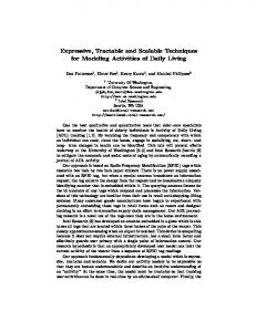
Figure 2. A cutset network

.7

c

b

.2

.8

b

.8

.2

c

b

c

.5

.5

.6

.4

.4

.6

.3

.7

b

b

b

b b

b b

b

(b) Figure 1. (a) A probability distribution, (b) An OR tree representing the distribution given in (a).

node l(x) corresponding to the assignment x and w(vi , vj ) is the probability value attached to the edge between vi and vj .

wiche, 2008) and context-specific independence (Boutilier et al., 1996) by branching on different variables at the same level (or depth) (Gogate & Domingos, 2010; Gogate et al., 2010). As a result, they can yield a compact representation, even if the size of the cutset is arbitrarily large. For example, consider the cutset network given in Fig. 2. The left most leaf node represents a tree Bayesian network over V \{a, e, f } while the right most leaf node represents a tree Bayesian network over V \ {a, b}. Technically, the size of the cutset, namely the subset of nodes which when conditioned on yield a tree network can be as large as the union of the variables mentioned at various levels in the OR tree. Thus, for the cutset tree given in Fig. 2, the size of the cutset can be as large as {a, b, e, f }.

4. Learning Cutset Networks 3. Cutset Networks Cutset Networks (CNets) are a hybrid of OR trees and tree Bayesian networks, with an OR tree at the top and a tree Bayesian network attached to each leaf node of the OR tree. Formally a cutset network is a pair C = (O, T) where O is an OR tree and T = {T1 , . . . , Tl } is a collection of tree networks. The distribution represented by a cutset network is given by:     Y P (x) =  w(vi , vj ) Tl(x) (xV (Tl(x) ) ) (vi ,vj )∈pathO (x)

(3) where pathO (x) is the path from the root to the unique leaf node l(x) corresponding to the assignment x, w(vi , vj ) is the probability value attached to the edge between vi and vj and Tl(x) is the tree Bayesian network associated with l(x) and V (Tl(x) ) is the set of variables over which Tl(x) is defined. Fig. 2 shows an example cutset network. Note that unlike classic cutset conditioning, cutset networks can take advantage of determinism (Chavira & Dar-

As mentioned in the introduction, if the size of the cutset is bounded by k, we can easily come up with a polynomial time algorithm for learning cutset networks: systematically search over all subsets of size k. Unfortunately, this naive algorithm is impractical because of its high polyomial complexity; the time complexity of this algorithm is at least Ω(nk+2 d) where n is the number of variables and d is the number of training examples. Therefore, in this section we will present an algorithm that uses techniques adapted from the decision tree literature to learn cutset networks. Simply put, given training data D = {x1 , . . . , xd } defined over a set V of variables, we can use the following recursive or divide-and-conquer approach to learn a cutset network from D (see Algorithm 1). Select a variable using the given splitting heuristic, place it at the root and make one branch for each of its possible values. Repeat the approach at each branch, using only those instances that reach the branch. If at any time, some pre-defined termination condition is satisfied, run the Chow-Liu algorithm on the remaining variables. It is easy to see that the optimal probability value, assuming that we are using the maximum likelihood esti-

Cutset Networks: A Simple, Tractable, and Scalable Approach for Improving the Accuracy of Chow-Liu Trees

Algorithm 1 LearnCNet Input: Training dataset D = {x1 , ..., xd }, Variables V . Output: A cutset network C

xv ∈∆v

if Termination condition is satisfied then return ChowLiuTree(D) end if Heuristically select a variable v ∈ V for splitting Create a new node Ov labeled by v. /* Each node has a left child Ov .lef t, a right child Ov .right, a left probability Ov .lp and a right probability Ov .rp. */ Let Dv=0 = {xi ∈ D|xiv = 0} Let Dv=1 = {xi ∈ D|xiv = 1} L| Ov .lp ← |D |D|

Given a closed-form expression for the entropy of the data, we can calculate the information gain or the expected reduction in the entropy after conditioning on a variable v using the following expression: b GainD (v) = H(D) −

where Dxv = {xi ∈ D : xiv = xv }. From the discussion above, the splitting heuristic is obvious: select a variable that has the highest information gain. 4.2. Termination Condition and Post-Pruning

mation principle, attached to each branch in the OR tree is the fraction of the instances at the parent that actually reach the branch. The two main choices in the above algorithm are which variable to split on and the termination condition. We discuss each of them in turn, next, followed by the algorithm to learn mixtures of cutset networks from data. 4.1. Splitting Heuristics Intuitively, we should split on a variable that reduces the expected entropy (or the information content) of the two partitions of the data created by the split. The hope is that when the expected entropy is small, we will be able to represent it faithfully using a simple distribution such as a tree Bayesian network. Unfortunately, unlike traditional classification problems, in which we are interested in (the entropy of) a specific class variable, estimating the joint entropy of the data when the class variable is not known is a challenging task (we just don’t have enough data to reliably measure the joint entropy). Therefore, we propose to approximate the joint entropy by the average entropy over individual variables. Formally, for our purposes, the entropy of data D defined over a set V of variables is given by:

v∈V

X |Dx | v b H(Dxv ) |D|

xv ∈∆v

R| Ov .rp ← |D |D| Ov .lef t ← LearnCNet(Dv=0 , V \ v) Ov .right ← LearnCNet(Dv=1 , V \ v) return Ov

1 X b H(D) = HD (v) |V |

where HD (v) is the entropy of variable v relative to D. It is given by: X P (xv )log(P (xv )) HD (v) = −

(4)

A simple termination condition that we can enforce is stopping when the number of examples at a node falls below a fixed threshold. Alternatively, we can also declare a node as a leaf node if the entropy falls below a threshold. Unfortunately, both these criteria are highly dependent on the threshold used. A large threshold will yield shallow OR trees that are likely to underfit the data (high bias) while a small threshold will yield deep trees that are likely to overfit the data (high variance). To combat this, inspired by the decision tree literature (Quinlan, 1986; 1993), we propose to use reduced error pruning. In reduced error pruning, we grow the tree fully and post-prune in a bottom-up fashion. (Alternatively, we can also prune in a top-down fashion). The benefits of pruning over using a fixed threshold are that it avoids the horizon effect (the thresholding method suffers from lack of sufficient look ahead). Pruning comes at a greater computational expense than threshold based stopped splitting and therefore for problems with large training sets, the expense can be prohibitive. For small problems, though, these computational costs are low and pruning should be preferred over stopped splitting. Moreover, pruning is an anytime method and as a result we can stop it at any time. Formally, our proposed reduced error pruning for cutset networks operates as follows. We divide the data into two sets: training data and validation data. Then, we build a full OR tree over the training data, declaring a node as a leaf node using a weak termination condition (e.g., the number of examples at a node is less than or equal to 5). Then, we recursively visit the tree in a bottom up fashion, and replace a node and the sub-tree below it by a leaf node if it increases the log-likelihood on the validation set. We summarize the time and space complexity of learning

Cutset Networks: A Simple, Tractable, and Scalable Approach for Improving the Accuracy of Chow-Liu Trees

(using Algorithm 1) and inference in cutset networks in the following theorem. Theorem 4.1. The time complexity of learning cutset networks is O(n2 ds) where s is the number of nodes in the cutset network, d is the number of examples and n is the number of variables. The space complexity of the algorithm is O(ns), which also bounds the space required by the cutset networks. The time complexity of performing marginal and maximum-a-posteriori inference in a cutset network is O(ns). Proof. The time complexity of computing the gain at each internal OR node is O(n2 d). Similarly, the time complexity of running the Chow-Liu algorithm at each leaf node is O(n2 d). Since there are s nodes in the cutset network, the overall time complexity is O(n2 ds). The space required to store an OR node is O(1) while the space required to store a tree Bayesian network is O(n). Thus, the overall space complexity is O(max(n, 1)s) = O(ns). The time complexity of performing inference at each leaf Chow-Liu node is O(n) while inference at each internal OR node can be done in constant time. Since the tree has s nodes, the overall inference complexity is O(ns). 4.3. Mixtures of Cutset Networks Similar to mixtures of trees (Meila & Jordan, 2000), we define mixtures of cutset networks as distributions of the form: k X P (x) = λi Ci (x) (5)

also update the mixture co-efficients using the following expression: Pd t j j=1 P (z = i|x ) t+1 λi = d We can run EM until it converges or until a pre-defined bound on the number of iterations is exceeded. The quality of the local maxima reached by EM is highly dependent on the initialization used and therefore in practice, we typically run EM using several different initializations and choose parameter settings having the highest log-likelihood score. Notice that by varying the number of mixture components, we can explore interesting bias versus variance tradeoffs. Large k will yield high variance models and small k will yield high bias models. We summarize the time and space complexity of learning and inference in mixtures of cutset networks in the following theorem. Theorem 4.2. The time complexity of learning mixtures of cutset networks is O(n2 dsktmax ) where s is the number of nodes in the cutset network, d is the number of examples, k is the number of mixture components, tmax is the maximum number of iterations for which EM is run and n is the number of variables. The space complexity of the algorithm is O(nsk), which also bounds the space required by the mixtures of cutset networks. The time complexity of performing marginal and maximum-a-posteriori inference in a mixtures of cutset networks is O(nks). Proof. Follows from Theorem 4.1

i=1

Pk with λi ≥ 0 for i = 1, . . . , k, and i=1 λi = 1. Each mixture component Ci (x) is a cutset network and λi is its mixture co-efficient. At a high level, one can think of the mixture as containing a latent variable z which takes a value i ∈ {1, . . . , k} with probability λi . Next, we present a version of the expectaton-maximization algorithm (EM) (Dempster et al., 1977) for learning mixtures of cutset networks from data. The EM algorithm operates as follows. We begin with random parameters. At each iteration t, in the expectation-step (E-step) of the algorithm, we find the probability of completing each training example, using the current model. Namely, for each training example xj , we compute λt C t (xj ) P t (z = i|xj ) = Pk i i t t j r=1 λr Cr (x ) Then, in the maximization-step (M-step), we learn each mixture component i, using a weighted training set in which each example j has weight P t (z = i|xj ). This yields a new mixture component Cit+1 . In the M-step, we

5. Empirical Evaluation The aim of our experimental evaluation is two fold: comparing the speed, measured in terms of CPU time, and accuracy, measured in terms of test-set log likelihood scores, of our methods with state-of-the-art methods for learning tractable models. 5.1. Methodology and Setup We evaluated our algorithms as well as the competition on 20 benchmark datasets shown in Table 1. The number of variables in the datasets ranged from from 16 to 1556, and the number of training examples varied from 1.6K to 291K examples. All variables in our datasets are binary-valued for a fair comparison with other methods, who operate primarily on binary-valued input. These datasets or a subset of them have also been used by (Davis & Domingos, 2010; Lowd & Rooshenas, 2013; Lowd & Davis, 2010; Gens & Domingos, 2013; Van Haaren & Davis, 2012). We implemented three variations of our algorithms: (1) learning CNets without pruning (CNet), (2) learning CNets

Cutset Networks: A Simple, Tractable, and Scalable Approach for Improving the Accuracy of Chow-Liu Trees Table 1. Runtime Comparison(in seconds). Time-limit for each algorithm: 48 hours. †indicates that the algorithm did not terminate in 48 hours. DATASET NLTCS MSNBC KDDC UP 2000 P LANTS AUDIO J ESTER N ETFLIX ACCIDENTS R ETAIL P UMSB - STAR DNA KOSAREK MSW EB B OOK E ACH M OVIE W EB KB R EUTERS -52 20N EWSGROUP BBC AD

VAR # 16 17 64 69 100 100 100 111 135 163 180 190 294 500 500 839 889 910 1058 1556

T RAIN 16181 291326 180092 17412 15000 9000 15000 12758 22041 12262 1600 33375 29441 8700 4524 2803 6532 11293 1670 2461

VALID 2157 38843 19907 2321 2000 1000 2000 1700 2938 1635 400 4450 32750 1159 1002 558 1028 3764 225 327

T EST 3236 58265 34955 3482 3000 4116 3000 2551 4408 2452 1186 6675 5000 1739 591 838 1540 3764 330 491

with pruning (CNetP) and (3) mixtures of CNets (MCNets). We compared their performance with the following algorithms from literature: learning sum-product networks with direct and indirect interactions (ID-SPN) (Rooshenas & Lowd, 2014), learning Markov networks using Airthmetic circuits (ACMN) (Lowd & Rooshenas, 2013), mixture of trees (MT) (Meila & Jordan, 2000), Chow-Liu trees (Chow & Liu, 1968), learning Sum-Product Networks (LearnSPN) (Gens & Domingos, 2013) and learning latent tree models (Choi et al., 2011). Most of the results on the datasets (except the results on learning Chow-Liu models) were made available to us by (Rooshenas & Lowd, 2014). They are part of the Libra toolkit available on Daniel Lowd’s web page. We smoothed all parameters using 1-laplace smoothing. For learning CNets without pruning, we stopped building the OR tree when the number of examples at the leaf node were less than 10. To learn MCNets and MTs, we varied the number of components from 5 to 20, in increments of 5 and ran the EM algorithm for 100 iterations or convergence whichever was earlier. 5.2. Accuracy Table 2 shows the test-set log likelihood scores for the various benchmark networks while Table 3 shows head-to-head comparison of all pairs of algorithms. We can see that MCNet has the best log-likelihood score on 11 out of the 20 benchmarks, while ID-SPN is the second best performing algorithm, with the best log-likelihood score on 8 out of the 20 benchmarks. In the head-to-head comparison, MC-

CN ET 0.156596 23.3985 94.5129 5.77256 15.9787 15.3571 22.3539 15.0001 22.6296 26.9437 7.67666 72.864 177.233 120.882 85.7481 200.211 485.221 1187.31 237.011 344.625

CN ET P 0.315338 47.1699 193.153 9.34513 18.9415 16.5981 22.6336 18.9098 26.6438 33.2207 6.26272 101.903 254.743 165.589 108.74 214.144 552.845 1209.23 236.602 392.876

MCN ET 38.6641 230.29 5483.83 306.532 630.663 660.153 796.501 735.546 948.853 1098.49 251.628 2828.90 6285.58 4799.62 3892.06 13073.60 36352.10 62769.70 6467.98 11883.1

ID-SPN 307.001 90354.00 38223.00 10590.00 14231.00 † † † 2116.01 18219.00 150850.00 † † 125480.00 78982.00 † † † 4157.00 285324.00

Nets is better than CNetP on all 20 benchmarks, ACMN on 16 benchmarks, MT on 18 benchmarks and LearnSPN on 17 benchmarks. CNetP is better than ID-SPN, ACMN and MT on 3 benchmarks while it is better than LearnSPN on 7 benchmarks. A careful look at the datasets reveal that when the number of training examples is larger, MCNet and to some extent CNetP are typically better than the competition. However, for small training set sizes, ID-SPN is the best performing algorithm. As expected, Chow-Liu trees and CNet are the worst-performing algorithms, the former underfits and the latter overfits. MCNet is consistently better than CNetP which suggests that whenever possible it is a good idea to use latent mixtures of simple models. This conclusion can also be drawn from the performance of MT, which greatly improves the accuracy of Chow-Liu trees. 5.3. Learning Time Table 1 shows the time taken by CNet, CNetP, MCNet and ID-SPN to learn a model from data. We gave a time limit of 48 hours to all algorithms and ran all our timing experiments on a quad-core Intel i7, 2.7 GHz machine with 8GB of RAM. The fastest algorithms in order are: CNet, CNetP, MCNet and ID-SPN. In fact, ID-SPN did not finish on 8 out of the 20 datasets in 48 hours (note that for the datasets on which ID-SPN did not finish in 48 hours, we report the test set log-likelihood scores from (Rooshenas & Lowd, 2014)).1 If we look at the learning time and accuracy as 1

We also ran ACMN on 17 out of the 20 datasets and observed that the time required by ACMN is comparable or larger than MC-

Cutset Networks: A Simple, Tractable, and Scalable Approach for Improving the Accuracy of Chow-Liu Trees Table 2. Test-set Log-Likelihood. †indicates that the results of this algorithm are not available. CN ET CN ET P MCN ET ID-SPN ACMN MT C HOWL EARN L IU SPN NLTCS -6.56 -5.89 -5.85 -6.02 -6.00 -6.01 -6.56 -6.11 MSNBC -6.43 -5.96 -5.95 -6.04 -6.04 -6.07 -6.43 -6.11 KDDC UP 2000 -2.28 -2.17 -2.12 -2.13 -2.17 -2.13 -2.28 -2.18 P LANTS -16.43 -13.12 -12.63 -12.54 -12.80 -12.95 -16.43 -12.98 AUDIO -46.83 -41.48 -39.45 -39.79 -40.32 -40.08 -43.81 -40.50 J ESTER -65.02 -54.73 -52.44 -52.86 -53.31 -53.08 -57.65 -53.48 N ETFLIX -70.41 -58.07 -56.00 -56.36 -57.22 -56.74 -59.64 -57.33 ACCIDENTS -37.78 -30.48 -29.23 -26.98 -27.11 -29.63 -33.01 -30.04 R ETAIL -12.11 -10.89 -10.78 -10.85 -10.88 -10.83 -10.90 -11.04 P UMSB - STAR -35.37 -24.14 -23.56 -22.40 -23.55 -23.71 -30.67 -24.78 DNA -115.18 -87.03 -84.85 -81.21 -80.03 -85.14 -87.24 -82.52 KOSAREK -12.11 -10.95 -10.58 -10.60 -10.84 -10.62 -11.46 -10.99 MSW EB -14.24 -9.89 -9.71 -9.73 -9.77 -9.85 -10.10 -10.25 B OOK -39.29 -36.74 -34.36 -34.14 -35.56 -34.63 -37.70 -35.89 E ACH M OVIE -75.25 -57.52 -52.40 -51.51 -55.80 -54.60 -64.65 -52.49 W EB KB -208.36 -161.44 -155.99 -151.84 -159.13 -156.86 -164.61 -158.20 R EUTERS -52 -133.74 -86.90 -86.17 -83.35 -90.23 -85.90 -96.73 -85.07 20N EWSGROUP -187.53 -160.89 -150.80 -151.47 -161.13 -154.24 -164.79 -155.93 BBC -295.86 -260.42 -257.36 -248.93 -257.10 -261.84 -261.31 -250.69 AD -69.24 -16.43 -15.93 -19.00 -16.53 -16.02 -16.42 -19.73 DATASET

LTM -6.49 -6.52 -2.18 -16.39 -41.90 -55.17 -58.53 -33.05 -10.92 -31.32 -87.60 -10.87 -10.21 -34.22 † -156.84 -91.23 -156.77 -255.76 †

Table 3. Head-to-head comparison of the number of wins (in terms of test-set log-likelihood score) achieved by one algorithm over another, for all pairs of the 6 best performing algorithms used in our experimental study. CN ET P MCN ET ID-SPN ACMN MT L EARN SPN

CN ET P 20 17 14 17 12

MCN ET 0 9 4 1 3

a whole, CNetP is the best performing algorithm, providing reasonably accurate results in quick time.

6. Summary and Future Work In this paper we presented cutset networks - a novel, simple and tractable probabilistic graphical model. At a high level, cutset networks are operational representation of Pearl’s cutset conditioning method, with an OR tree modeling conditioning (at the top) and a tree Bayesian network modeling inference over trees at the leaves. We developed an efficient algorithm for learning cutset networks from data. Our new algorithm uses a decision-tree inspired learning algorithm for inducing the structure and parameters of the OR tree and the classic Chow-Liu algorithm for learning the tree distributions at the leaf nodes. We also presented an EMbased algorithm for learning mixtures of cutset networks. Our detailed experimental study on a variety on benchmark datasets clearly demonstrated the power of cutset netNet.

ID-SPN 3 11 3 3 0

ACMN 5 16 16 12 5

MT 3 19 16 8 4

L EARN SPN 8 17 20 15 16 -

works. In particular, our new algorithm that learns mixtures of cutset networks from data, was the best performing algorithm in terms of log-likelihood score on 55% of the benchmarks when compared with 5 other state-of-theart algorithms from literature. Moreover, our new one-shot algorithm, which builds a cutset network using the information gain heuristic and employs reduced-error pruning is not only fast (as expected) but also reasonably accurate on several benchmark datasets. This gives us a spectrum of algorithm for future investigations: fast, accurate one-shot algorithms and slow, highly accurate iterative algorithms based on EM. Future work includes learning polytrees having at most w parents at the leaves yielding w-cutset networks; using AND/OR trees or sum-product networks instead of OR trees yielding AND/OR cutset networks (Dechter & Mateescu, 2007); introducing structured latent variables in the mixture model; and merging identical sub-trees while learning to yield a compact graph-based representation.

Cutset Networks: A Simple, Tractable, and Scalable Approach for Improving the Accuracy of Chow-Liu Trees

ACKNOWLEDGEMENTS This research was partly funded by ARO MURI grant W911NF-08-1-0242, by the AFRL under contract number FA8750-14-C-0021 and by the DARPA Probabilistic Programming for Advanced Machine Learning Program under AFRL prime contract number FA8750-14-C-0005. The views and conclusions contained in this document are those of the authors and should not be interpreted as representing the official policies, either expressed or implied, of DARPA, AFRL, ARO or the US government.

References Bach, F.R. and Jordan, M.I. Thin junction trees. Advances in Neural Information Processing Systems, 14:569–576, 2001.

Gens, R. and Domingos, P. Learning the structure of sumproduct networks. In Proceedings of the Thirtieth International Conference on Machine Learning. JMLR: W&CP 28, 2013. Gogate, V. and Domingos, P. Formula-Based Probabilistic Inference. In Proceedings of the Twenty-Sixth Conference on Uncertainty in Artificial Intelligence, pp. 210– 219, 2010. Gogate, V., Webb, W., and Domingos, P. Learning efficient Markov networks. In Proceedings of the 24th conference on Neural Information Processing Systems (NIPS’10), 2010. Koller, D. and Friedman, N. Probabilistic Graphical Models: Principles and Techniques. MIT Press, Cambridge, MA, 2009.

Boutilier, C., Friedman, N., Goldszmidt, M., and Koller, D. Context-specific independence in Bayesian networks. In Proceedings of the Twelfth Conference on Uncertainty in Artificial Intelligence, pp. 115–123, Portland, OR, 1996. Morgan Kaufmann.

Lowd, D. and Davis, J. Learning Markov network structure with decision trees. In Proceedings of the 10th IEEE International Conference on Data Mining (ICDM), pp. 334–343, Sydney, Australia, 2010. IEEE Computer Society Press.

Chavira, M. and Darwiche, A. On probabilistic inference by weighted model counting. Artificial Intelligence, 172 (6-7):772–799, 2008.

Lowd, D. and Rooshenas, A. Learning Markov networks with arithmetic circuits. In Proceedings of the Sixteenth International Conference on Artificial Intelligence and Statistics (AISTATS 2013), Scottsdale, AZ, 2013.

Chechetka, A. and Guestrin, C. Efficient principled learning of thin junction trees. In Platt, J.C., Koller, D., Singer, Y., and Roweis, S. (eds.), Advances in Neural Information Processing Systems 20. MIT Press, Cambridge, MA, 2008. Choi, M. J., Tan, V., Anandkumar, A., and Willsky, A. Learning latent tree graphical models. Journal of Machine Learning Research, 12:1771–1812, May 2011. Chow, C. K. and Liu, C. N. Approximating discrete probability distributions with dependence trees. IEEE Transactions on Information Theory, 14:462–467, 1968. Darwiche, A. Modeling and reasoning with Bayesian networks. Cambridge University Press, 2009. Davis, J. and Domingos, P. Bottom-up learning of Markov network structure. In Proceedings of the Twenty-Seventh International Conference on Machine Learning, pp. 271–278, Haifa, Israel, 2010. ACM Press. Dechter, Rina and Mateescu, Robert. And/or search spaces for graphical models. Artificial intelligence, 171(2):73– 106, 2007. Dempster, A. P., Laird, N. M., and Rubin, D. B. Maximum likelihood from incomplete data via the EM algorithm. Journal of the Royal Statistical Society, Series B, 39:1– 38, 1977.

Meila, M. and Jordan, M. Learning with mixtures of trees. Journal of Machine Learning Research, 1:1–48, 2000. Mitchell, T. M. Machine Learning. McGraw-Hill, New York, NY, 1997. Narasimhan, Mukund and Bilmes, Jeff. Pac-learning bounded tree-width graphical models. In Proceedings of the Twentieth Conference on Uncertainty in Artificial Intelligence, 2004. Pearl, J. Probabilistic Reasoning in Intelligent Systems: Networks of Plausible Inference. Morgan Kaufmann, San Francisco, CA, 1988. Quinlan, J. R. Induction of decision trees. Machine Learning, 1:81–106, 1986. Quinlan, J. R. C4.5: Programs for Machine Learning. Morgan Kaufmann, San Mateo, CA, 1993. Rooshenas, A. and Lowd, D. Learning sum-product networks with direct and indirect interactions. In Proceedings of the Thirty-First International Conference on Machine Learning, Beijing, China, 2014. ACM Press. Van Haaren, Jan and Davis, Jesse. Markov network structure learning: A randomized feature generation approach. In AAAI, 2012.