Cutwidth of split graphs and threshold graphs∗ Pinar Heggernes†
Daniel Lokshtanov†
Rodica Mihai†
Charis Papadopoulos‡
Abstract We give a linear-time algorithm to compute the cutwidth of threshold graphs, thereby resolving the computational complexity of cutwidth on this graph class. Threshold graphs are a well-studied subclass of interval graphs and of split graphs, both of which are unrelated subclasses of chordal graphs. To complement our result, we show that cutwidth is NPcomplete on split graphs, and consequently also on chordal graphs. The cutwidth of interval graphs is still open, and only very few graph classes are known so far on which polynomialtime cutwidth algorithms exist. Thus we contribute to define the border between graph classes on which cutwidth is polynomially solvable and on which it remains NP-complete.
1
Introduction
The cutwidth problem asks, given a graph G, and a positive integer k, whether there exists a linear layout of the vertices of G so that any line inserted between two consecutive vertices of the layout cuts (intersects with) at most k edges. The cutwidth of the input graph is the smallest integer for which the question can be answered positively. This important graph layout problem was first proposed as a model to minimize the number of channels in a circuit [1, 19], and more recently it has found applications in areas like protein engineering [3], network reliability [15], automatic graph drawing [21], information retrieval [4], and as a subroutine in the cutting plane algorithm for TSP [14]. Like many other interesting graph problems, cutwidth is NP-complete [8], even when input graphs are restricted to planar graphs of maximum degree three [20], unit disk graphs, partial grids [9], and consequently bipartite graphs. Coping with the NP-completeness of the problem has been mainly channelled via approximation algorithms and fixed parameter algorithms. There is a polynomial-time O(log2 n)approximation algorithm for general graphs [17], and a polynomial-time constant factor approximation algorithm for dense graphs [2]. The best known parameterized algorithm for cutwidth so far runs in linear time (but of course exponential in the parameter k) [22]. Polynomial-time algorithms for the exact computation of cutwidth are known only for very few graph classes. For certain trivial graph classes, like meshes or complete p-partite graphs, there exist closed formulas for their cutwidth [10]. Cutwidth of proper interval graphs has a trivial solution following an interval ordering of the vertices [25]. The cutwidth of trees can ∗
This work is supported by the Research Council of Norway through grant 166429/V30. A preliminary version of this work was presented at WG 2008. † Department of Informatics, University of Bergen, N-5020 Bergen, Norway. Emails:
[email protected],
[email protected],
[email protected] ‡ Department of Mathematics, University of Ioannina, GR-45110 Ioannina, Greece. Email:
[email protected]
1
be computed in O(n log n) time by a sophisticated and technical algorithm [24] (see also [6]). The cutwidth of graphs having bounded treewidth and maximum degree, can be computed in polynomial time by advanced methods [23]. The computational complexity of cutwidth on threshold graphs has been open until now [10]. In this paper, we present an O(n)-time algorithm for computing the cutwidth of threshold graphs with n vertices. Threshold graphs are a well-studied graph class with a variety of theoretical applications [18], and they are both split graphs and interval graphs [5, 12]. Split and interval graphs are two unrelated subclasses of the widely-known class of chordal graphs. Before presenting our algorithm for threshold graphs, we show that the cutwidth problem remains NP-complete on split graphs (even on a very restricted type of split graphs), and hence also on chordal graphs. Our findings are summarized in Figure 1. split NPC chordal NPC
threshold P interval ?
Figure 1: The graph classes studied in this paper, and the complexity of cutwidth on each class according to our results. P means polynomial and NPC means NP-complete. The arrow represents the subset relation. The algorithm that we present for threshold graphs is simple and intuitive, and its execution does not at all depend on properties of threshold graphs; thus it can also be run on general graphs as a heuristic. Interestingly, while the algorithm correctly computes the cutwidth of threshold graphs, it does not compute the cutwidth of any known superclass or closely related class, like trivially-perfect graphs and chain graphs1 . For the proof of correctness of this algorithm on threshold graphs, we study the properties of a possible minimal counterexample through a series of structural results, and we show that the assumption of the existence of such a counterexample leads to a contradiction.
2
Preliminaries
We consider labeled undirected finite graphs with no loops or multiple edges. For a graph G = (V, E), we denote its vertex and edge set by V and E, respectively, with n = |V |. Every vertex v ∈ V has a distinct label, label(v), between 1 and n. We say that a vertex u is smaller than v if label(u) < label(v). For a vertex subset S ⊆ V , the subgraph of G induced by S is denoted by G[S]. Moreover, we denote by G − S the graph G[V \ S] and by G − v the graph G[V \ {v}]. In this paper, we distinguish between subgraphs and induced subgraphs. By a subgraph of G we mean a graph G′ on the same vertex set containing a subset of the edges of G, and we denote it by G′ ⊆ G. If G′ contains a proper subset of the edges of G, we write G′ ⊂ G. We write G − uv to denote the graph (V, E \ {uv}). 1
For completeness, we give small examples illustrating this fact in an appendix at the end of the paper.
2
The neighborhood of a vertex x of G is NG (x) = {v | xv ∈ E}. The closed neighborhood of x is ∆G (x) = |NG (x)|. If S ⊆ V , then NG (S) = S NG [x] = NG (x) ∪ {x}. The degree of x is G / S}, and the cut x∈S NG (x) \ S. We define the cut of S to be δ (S) = {uv ∈ E | u ∈ S, v ∈ size of S to be dG (S) = |δG (S)|. Vertex x is universal if NG [x] = V and isolated if NG (x) = ∅. We will omit the subscripts and superscripts when there is no ambiguity. A graph is connected if there is a path between any pair of vertices. A connected component of a disconnected graph is a maximal connected subgraph of it. A clique is a set of pairwise adjacent vertices, while an independent set is a set of pairwise non-adjacent vertices. Given a graph G = (V, E), a layout L is a one-to-one mapping L : V → {1, . . . , n}. We will also denote a layout L by hv1 , v2 , · · · vn i such that L(vi ) = i. For an integer i between 1 and n we define the set Vi to be {v1 , · · · , vi }. We say that u is before v in L, or u ∆(vi ) then vi := v Vi := Vi−1 ∪ {vi }; L(vi ) := i;
To illustrate the algorithm by an example, in Figure 2 (a) we depict a threshold graph on three levels with the corresponding label on each vertex. Execution of the Algorithm MinCut on this graph is given in Figure 2 (b) while the computed layout is shown in Figure 2 (c). Before reaching the details of why Algorithm MinCut produces optimal layouts when the input is a threshold graph, we need to study how the layouts produced by the algorithm look. Observe first that if G has isolated vertices, then these can be placed in arbitrary positions in any optimal cutwidth layout, and our algorithm places them in the beginning of the output layout. For the statements of the following results in this section, we let L = hv1 , . . . , vn i be the layout computed by Algorithm MinCut when run on a threshold graph G with threshold partition (C1 , . . . , Cℓ , I1 , . . . , Iℓ ). One should notice that in a threshold graph, two vertices with the same degree have the same open neighborhood if they are nonadjacent and the same closed neighborhood if they are adjacent. Thus, in threshold graphs, the labels of the vertices do not really affect the layout 5
produced by Algorithm MinCut, because whether or not there is an edge between vi and vj for 1 ≤ i < j ≤ n is independent of the labels of the vertices, and depends only on which sets of the threshold partition they belong to. The reason we include the labels in the description of the algorithm is that the labels simplify the discussions in the proofs. One should note that the labels do indeed affect the layout produced by the algorithm if the algorithm is run on a graph
C1
v1
v6
v2
I1
v7
C2
v3 v8
I2
v4
C3
v9
v5
I3
(a)
step
1
v1
v2
v3
v4
1
1
3
4
rank v5 4
sele tion
v6
v7
v8
v9
8
6
6
5
v1
3
4
4
6
6
6
5
v2
3
4
4
4
6
6
5
v3
4
4
4
2
4
4
5
v6
5
2
2
2
2
3
v4
6
2
0
0
1
v7
7
0
-2
-1
v8
8
-2
-3
v9
9
-4
1
2 3
v5 (b)
v1
v2
v3
v6
v4
v7
v8
v9
v5
( )
Figure 2: (a) A threshold graph on three levels where each vertex is labeled according to a preprocessing step. (b) Steps of the Algorithm MinCut applied on the threshold graph. (c) A layout of cutwidth 9 produced by the algorithm.
6
that is not a threshold graph. Given two vertices u and v of G such that u ∈ I and v ∈ C, we define the vertex set over(u, v) to contain all vertices x ∈ I such that label(x) < label(u) and all vertices y ∈ C such that label(y) < label(v). The essence of the following lemma is that the algorithm picks vertices at lower levels before proceeding to higher levels, and that it starts with a vertex of I. Lemma 4.1. For any i ∈ {1, . . . , n} and k ∈ {1, . . . , ℓ}: (a) If Vi ∩ Ik 6= ∅, then Ik′ ⊆ Vi , for every 1 ≤ k′ < k. (b) If Vi ∩ Ck 6= ∅, then Ck′ ⊆ Vi , for every 1 ≤ k′ < k. (c) If Vi ∩ Ik = ∅, then Vi ∩ Ck = ∅. Proof. We prove all the statements simultaneously by induction on i. Vertex v1 is of minimum degree and hence v1 ∈ I1 , so for i = 1 the statements are trivially true. Assume now that all three statements hold whenever i < r and consider the r’th step of the algorithm. We first prove that (a) must be true for i = r. It suffices to show that if vr ∈ I, then vr is a vertex with the lowest degree out of the ones that are not in Vr−1 . Indeed, consider two vertices u and v ∈ I \ Vr−1 such that ∆(u) < ∆(v). Since level(v) > level(u), because (c) holds for Vr−1 by the induction hypothesis, every neighbor of v that is not a neighbor of u is not in Vr−1 . Thus rankVr−1 (u) < rankVr−1 (v) and (a) follows for i = r. We prove that (b) is true for i = r; that is, if vr ∈ C, then vr is a vertex with the highest degree out of the ones that are not in Vr−1 . Let t be the largest integer such that Vr−1 ∩ It 6= ∅. For a vertex u ∈ Ct′ with t < t′ , let v be a vertex in It′ . Because (c) holds for Vr−1 by the induction hypothesis, v ∈ / Vr−1 and rankVr−1 (v) ≤ rankVr−1 (u). Additionally, label(v) < label(u) and so the algorithm would not pick vr to be u. Furthermore, for every two vertices u and v in C \ Vr−1 such that level(u) < level(v) ≤ t, it follows that every neighbor of u that is a nonneighbor of v is in Vr−1 , yielding rankVr−1 (u) < rankVr−1 (v) and completing the proof of (b) for i = r. Finally, we prove that (c) is true for i = r. Consider a level t such that It ∩ Vr−1 = Ct ∩ Vr−1 and let u ∈ It and v ∈ Ct . Since (a) and (b) are true for r − 1, every neighbor of v that is not a neighbor of u is not in Vr−1 . Unless t = ℓ and |Iℓ | = 1, ∆(u) < ∆(v) so rankVr−1 (u) < rankVr−1 (v). If t = ℓ and |Iℓ | = 1, then u and v have the same closed neighborhood, but label(u) < label(v). In both cases u