CVD2014 - A database for evaluating no-reference ...

IEEE TRANSACTION ON IMAGE PROCESSING, VOL. XX, NO. XX, XXXX XXXX

1

CVD2014 - A database for evaluating no-reference video quality assessment algorithms Mikko Nuutinen, Toni Virtanen, Mikko Vaahteranoksa, Tero Vuori, Pirkko Oittinen, and Jukka Häkkinen

Abstract—In this study, we present a new video database: CVD2014 - Camera Video Database. In contrast to previous video databases, this database uses real cameras rather than introducing distortions via post-processing, which results in a complex distortion space in regard to the video acquisition process. CVD2014 contains a total of 234 videos that are recorded using 78 different cameras. Moreover, this database contains observer-specific quality evaluation scores rather than only providing mean opinion scores. We have also collected openended quality descriptions that are provided by the observers. These descriptions were used to define the quality dimensions for the videos in CVD2014. The dimensions included sharpness, graininess, color balance, darkness and jerkiness. At the end of this paper, a performance study of image and video quality algorithms for predicting subjective video quality is reported. For this performance study, we proposed a new performance measure that accounts for observer variance. The performance study revealed that there is room for improvement regarding the video quality assessment algorithms. The CVD2014 video database has been made publicly available for the research community. All video sequences and corresponding subjective ratings can be obtained from the CVD2014 project page (http: //www.helsinki.fi/psychology/groups/visualcognition/). Index Terms—Video camera, quality attribute, subjective evaluation, video quality algorithm

I. I NTRODUCTION

T

HE research field related to image and video quality is multidisciplinary and is composed of the primary disciplines of vision, color, computational and behavioral sciences. Among the top priorities of this research is the development of a computational model (in the form of an algorithm) that is capable of predicting the subjective visual quality of natural images and videos. An established practice is to use publicly available databases when the performance of new image or video quality assessment (I/VQA) algorithms are tested or validated. These databases include test images or videos that are distorted in different ways and annotated with subjective ratings. Table I lists the publicly available video databases known M. Nuutinen was with the Department of Media Technology, Aalto University, Espoo, Finland. He is now with the Institute of Behavioural Sciences, University of Helsinki, Helsinki, Finland e-mail: [email protected]. T. Virtanen and J. Häkkinen are with the Institute of Behavioural Sciences, University of Helsinki, Helsinki, Finland e-mail: [email protected], [email protected] M. Vaahteranoksa is with Microsoft Co. Espoo, Finland e-mail: [email protected], [email protected] T. Vuori was with Microsoft Co. Espoo, Finland. He is now with Intel Co. Tampere, Finland e-mail: [email protected] P. Oittinen is with the Department of Computer Science, Aalto University, Espoo, Finland e-mail: [email protected] Manuscript received March 27, 2015; revised XXXX XX, XXXX.

TABLE I: Public video databases and distortion types Database EPFL-PoliMi [5] ECVQ and EVVQ [6] Poly@NYU Video Quality Databases [7], [8] Poly@NYU Packet Loss Database [9] IRCCyN/IVC databases [10] LIVE [11] LIVE Mobile [12] MMSP (SVD) [13] CSIQ [14] IVP [15] TUM 1080p25 [16] TUM 1080p50 [17] AVC HD Database [18] VQEG FR-TV Phase I Database [19] VQEG HDTV Database [20]

Distortions Transmission error Compression Frame rate, quantization parameter Transmission error

Data Raw DMOS + σ Raw

Compression, Transmission error Compression, transmission error Compression, transmission error Spatial and temporal resolution, compression Compression, transmission error Compression, transmission error Compression Compression Transmission error Compression, transmission error Compression, transmission error

Raw

Raw

DMOS + σ DMOS + σ Raw DMOS + σ DMOS + σ Raw Raw Raw DMOS + σ Raw

to us. Note that not all of the distortions that occur in the typical video production chain are included in these databases. The traditional video production chain can be divided into video acquisition, encoding and transmission processes [1]. Furthermore, there can be a fourth process, rendering, which is the key aspect of three-dimensional (3D) and high dynamic range (HDR) video production [2]–[4]. The distortions in the public databases presented in Table I are related to the encoding (compression) and transmission processes, but they are not related to video acquisition or rendering. The focus of this study is to present a new database related to video acquisition. Thus, we argue that the VQA algorithms proposed in the literature and validated by using public video databases (such as those listed in Table I) are only feasible with a restricted set of distortions. One reason why the process of video acquisition is missing from the databases is because the video samples from it are cumbersome to produce. Capturing real video samples that use different video cameras, which we have performed in this study, requires a considerable amount of work. In addition, a large number of different video cameras should be available. Another option to produce samples is to simulate the video capturing process. In the video capturing process, the camera optics project an optical image onto an image sensor [21], while signal processing

2

tunes the capturing parameters (exposure and focus). Then, for example, white balance, sharpness, noise reduction and colors are processed [22]–[24] before the output is encoded. The simulation is, however, complex and has not yet matured as a research topic. Note that prior work regarding the quality of video acquisition is related more to the camera quality research field than to the field of signal processing (I/VQA algorithms). In the camera quality research field, both subjective and objective methods have long traditions. Subjective evaluations function as the ground truth for camera quality [25]–[30]. Subjective methods have also been used for characterizing the quality properties of photographs and video sequences [31]–[33]. For example, Radun et al. [32] found that the most important image quality dimensions are color shift, naturalness, darkness and sharpness. However, subjective measurements require a large number of assessors and are time consuming to implement. In addition, subjective measurements cannot be used for applications that require real-time parametric control based on quality data. Methods for objective measurements in camera quality research employ synthetic test target charts rather than images or video sequences captured from natural scenes. Test targets are captured under specific types and levels of illumination in a strict laboratory environment, and characterization values are computed from the acquired signal. The ISO (International Organization for Standardization) has published objective camera measurement standards for resolution [34], noise [35], lens optical distortion [36], Opto-Electrical Conversion Function (OECF) [37] and color [38] characterization and measurements. Test target measurements, however, primarily describe how camera systems function. They do not correlate well with the perceived quality of images and video sequences captured from natural scenes [39]. In addition, adaptive signal processing in cameras hinders the interpretation of measurement data [40]–[43]. I/VQA algorithms (e.g., [44]–[52]) have been developed for measuring the perceived quality of natural images and videos. Unfortunately, the current VQA algorithms, as stated above, and IQA algorithms, as indicated in [53], have been developed only for the processes of image/video encoding and transmission. A VQA algorithm developed for the process of video acquisition could substitute or supplement test target measurements in the field of camera quality research. In this paper, we propose the CVD2014 video database, which is, to the best of our knowledge, the first publicly available video database in which there are distortions that arise from the video acquisition process. The primary purpose of CVD2014 is to function as training data for developing new VQA algorithms dedicated to the video acquisition process. The videos in CVD2014 were captured using 78 different cameras. The quality of the cameras varied from low-quality mobile phone cameras to dedicated video and high-quality digital single lens reflex (DSLR) cameras. The videos were evaluated through subjective experiments. In addition to overall quality, we collected quality attribute scales and open-ended quality descriptions. The video database and experimental data have been made publicly available for the research community. In


addition, we distribute all of the subjective data rather than making only the mean opinion scores available. The remainder of this paper is divided into three parts. In the first part, we describe the properties of the capturing devices and captured scenes and how the videos were processed for the subjective experiments. The second part introduces the subjective experiment settings and how the subjective data were analyzed. The third part of the paper presents the performance study of the video quality assessment algorithms. For that part of the study, we have proposed a new measure for evaluating algorithms. This new performance measure accounts for the observer variance, which is possible with the CVD2014 database because observer-specific data are available. The primary contributions of this paper are summarized below: •

•

The videos in the CVD2014 database are captured using 78 different cameras, and the distortions are related to the video acquisition process. In contrast to many earlier databases, the videos in the CVD2014 database contain audio. In addition, the CVD2014 database contains more comprehensive and detailed subjective data. We have analyzed subjective quality attributes and open-ended descriptions collected from the observers. For the algorithm performance study, we introduced a new performance measure that accounts for the variance between observer answers. In earlier studies, the predictions of the algorithms were only compared to the mean opinion scores. II. V IDEO SEQUENCES , CAPTURING AND POST- PROCESSING

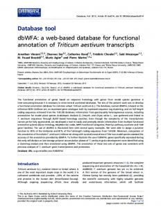
A. Video sequences The challenge of constructing the CVD2014 database was that the video sequences need to be shot by different cameras and still be as similar as possible. When the earlier video databases were constructed, they only needed to capture one good video sequence for one scene. Then, the entire set of test videos was processed from the reference. Because the quality differences between the video sequences in the CVD2014 database arise from the different capturing devices (see Section II-B), the test videos had to be captured one at a time when using different cameras. The video sequences in the CVD2014 database were captured from many different scenes. Figure 1 shows three frames from the scenes. The frames are from the beginning, middle and end of the video sequences. The length of the trimmed and processed videos was 10 - 25 s. The processing steps of the videos for the subjective experiments and algorithm performance study are described in Section II-D. Short descriptions of the sequences are provided below. •

•

Traffic – A bus is driving on a busy road and passes the camera. The camera pans to the direction of the sea where a man is walking on a walkway. City – A view from a central location in a city where a man is walking from the outdoors to a tunnel, which includes a gradual change in color temperature and

NUUTINEN et al.: CVD2014 - A DATABASE FOR EVALUATING NO-REFERENCE VIDEO QUALITY ASSESSMENT ALGORITHMS

3

Fig. 2: Spatial and temporal activity presented as point cloud values for the example (high-quality) video sequences

Fig. 1: CVD2014 video database sequences 1-5 (from top to bottom): Traffic (1), City (2), Talking Head (3), Newspaper (4) and Television (5)

• • •

illuminance based on the panning camera and moving objects. Talking Head – The upper body of a man who is talking (in Finnish). Newspaper – A man is reading a newspaper indoors, and the light turns to a different color temperature. Television – A man is walking to a sofa and picks up an orange from a basket, sits down and switches on a TV, on which a news program begins.

The scenes contain different amounts of spatial and temporal information. ITU (International Telecommunication Union) Recommendation P.910 [26] defines the metrics of spatial perceptual information (SI) and temporal perceptual information (TI) for characterizing the level of activity in a video sequence. The calculation of SI in each frame f (x, y, t) of a video sequence is filtered by a Sobel filter, and the standard deviation std(Sobel(f (x, y, t))) for each Sobel-filtered frame is calculated when x and y are pixel coordinates and t is a frame index. TI is based on the difference between successive frames, D(x, y, t) = f (x, y, t) − f (x, y, t + 1). The standard deviation std(D(x, y, t)) of each difference frame is calculated. The standard [26] defines that the SI and TI values for a video sequence are the maximums of std(Sobel(f (x, y, t))) and std(D(x, y, t)), respectively. We were concerned that a single SI or TI value, as described in the standard, for the entire video sequence could be misleading if the content changes throughout the duration of the video. For example, in the videos in the CVD2014 database, there are moving and static objects, and videos are captured using static or panning cameras in a row. Thus, we decided to use the point clouds of SI and TI values, rather

than their single values, when characterizing the scenes from which the videos were captured. Point clouds characterize the time course properties of the videos better than single values. Figure 2 shows the point cloud values (SI(t), T I(t − 1)) of the CVD2014 scenes, where t = 2, ..., T and T is the number of frames in the video sequence. The values were calculated from the high-quality video sequences. The point clouds show that the motion and detail levels vary for the different scenes. For example, both the SI and TI values in the talking head scene are low and at a constant level throughout the scene. With the newspaper and traffic scenes, the TI values vary slightly throughout the scenes, but the SI values remain at a constant level. With the television and city scenes, both the SI and TI levels vary considerably, which indicates the presence of spatial and temporal properties that vary considerably. B. Video capturing and artifacts In total, 3 DSLR, 4 digital video (DVC), 8 digital still (DSC) and 63 mobile cameras were used for video capturing. Each camera was used in auto mode. Different cameras have different recording formats, settings and video codecs. The cameras used the H.264 (43 cameras), MPEG-4 (28 cameras), MPEG-2 (3 cameras), MJPG (2 cameras) or DV (2 cameras) codecs for compressing video streams. Frequency data of different video formats1 and frame rates are listed in Table II. The videos in the CVD2014 database, which were produced by 78 different capturing devices, contain multiple highly complex and signal-dependent artifacts, unlike most distortions in the earlier video databases. These distortions are very difficult to simulate because they are not only dependent on the optical systems of the capturing devices but also on the signal processing and sensor characteristics. The raw signal from a sensor includes artifacts, such as photon noise, thermal noise, pixel defects, pixel saturation and spatial under-sampling. A low temporal sampling rate results in a jerkiness artifact, which can be perceived as discontinuities of movements. The optics introduce several optical aberrations, such as lens shading and geometrical distortions. 1 Common Intermediate Format (CIF), Quarter CIF (QCIF), Video Graphics Array (VGA), Quarter VGA (QVGA), National Television System Committee (NTSC), Phase Alternating Line (PAL), Wide PAL (WPAL), High Definition (HD), Full HD (FHD)

4


TABLE II: Frequency table of video formats and frame rates in the cameras used for capturing the videos in the CVD2014 database

Video format QCIF (176 x144) QVGA (320 x 240) CIF (352 x 288) VGA (640 x 480) NTSC (720 x 480) PAL (768 x 576) WPAL (848 x 480) HD (1280 x 720) FHD (1920 x 1080)

10< f ps ≤13

13< f ps ≤16 1

19< f ps ≤22

22< f ps ≤25

25< f ps ≤28

1

28< f ps ≤31 1

1 7 1

1 3 1 8 6

1

18 2

1 1

9 15

reproduction and signal sharpening [34], [40]–[42]. The IQAnalyzer software (v. 5.2.7) was used for the analyses. Figure 4 shows the histograms of the SNR and MTF values of the capturing devices for an illumination level of 1000 lux. The illumination level of 1000 lux is typical outdoor lighting conditions. From the histograms, it can be observed that the measured values vary, which indicates the varying quality of the cameras. Video sequences with different quality levels are very important if video databases are to be used for the development of VQA algorithms and benchmarking tasks. Test target data and analysis with more details can be found on the CVD2014 project page. D. Video post-processing

The signal control adjusts the 3A of the camera: auto-focus (AF), auto-exposure (AE) and automatic white balance (AWB) algorithms [33]. A failed exposure or a failed focus induce dark or overexposed video and loss in detail and sharp edges. Global color errors, such as a green, red or yellow shade in the final video, are often caused by unsuccessful AWB. Signal processing is divided into dedicated sequential blocks, and each block is tuned depending on characteristics of the sensor and optics [22]. According to [22], [23], typical operations are defective pixel correction, noise removal, black level adjustment and color correction. De-mosaicking is the process of interpolating missing color filter array-sampled pixel values. Finally, a compression algorithm is applied on the digital video stream. The key principle of video compression is to eliminate spatial and temporal redundancy without visible artifacts. Typical artifacts are, e.g., blocking, basis image effect, staircase effect, ringing effect, motion compensation mismatch and mosquito effect [54]. Figure 3 shows typical frames from the video samples in the CVD2014 database. The figure caption contains qualitative descriptions for these video samples. The descriptions are collected by the method explained in Section III. According to the descriptions, the samples in Figs. 3a and 3d are sharp and bright. The sample in Fig. 3b is grainy because of sensor noise and/or compression artifacts. The samples in Figs. 3c and 3e are unsharp and yellow or reddish because of spatial under-sampling or failed AF and AWB. The sample in Fig. 3f is grainy and shivery because of compression artifacts, such as mosquito and ringing effects. In addition, a staircase effect can be identified from the fence in Fig. 3f. C. Characterization of capturing devices In addition to test scene capturing, we obtained standard test target measurements for the cameras. We measured the modulation transfer function (MTF) and signal-to-noise ratio (SNR) metrics. Modulation transfer was measured by spatial frequency response (SFR) [34] from the slanted edge area of the MICA test target [55]. SNR [35] was measured from the gray patches of the MICA test target, from which the ratio of the average signal value to the standard deviation of the signal value was calculated. The SNR value indicates the noise level as well as noise reduction processing. The MTF value (line pairs per picture height, LP/PH) indicates detail

For the subjective experiments (Section III), the videos were post-processed to the spatial format of VGA (640x480 pixels) or HD (1280x720 pixels) using the Avisynth script language (v. 2.5) and VirtualDub (v. 1.10.4). The frame-rates were maintained at their original values. The audio volume of the videos was normalized using Audacity software (v. 2.0.5). Note that we used these same post-processed videos for the performance evaluation of the algorithms (Section V). The original videos were opened in VirtualDub using the ’DirectShowSource’ command. If the video resolution was different than VGA or HD, it was scaled using the ’BicubicResize’ command. The videos in the CVD-I database are in VGA format, and the videos in the CVD-II and CVD-III databases are in HD format2 . If the aspect ratio of the original video differed from that of the target, it was cropped to the correct aspect ratio using the ’crop’ command. For example, with the VGA format, the aspect ratio should be 3/2, and with the HD format, it should be 16/9. If the video resolution was lower than 720 lines (SD video), the color space of the video was transformed to the color space of HD video using the ’ColorMatrix(mode=”rec.601→Rec.709”)’ command. When the video was opened in VirtualDub, the audio track was extracted to uncompressed WAV format and normalized in Audacity. Note that audio was captured directly by the camera and that normalization was performed because different cameras can record audio at different volumes. By normalizing the audio, we avoided the observers having to tune the video volume settings between different test videos. For the normalization process, the maximum amplitude value was set to -3 dB, the number of audio channels was maintained constant (1=mono or 2=stereo) and sampling rate was set to 48 kHz. Finally, the videos were trimmed to the same lengths in terms of content such that all of the test videos began from and ended on the same actions. The videos were compressed using the lossless HuffYUV compression with the YUY2 color space, and they were deposited in the AVI containers. III. S UBJECTIVE EXPERIMENTS The CVD2014 database is divided into four parts or subdatabases. The sub-databases are named CVD-I, CVD-II, 2 The CVD2014 database is divided into the CVD-I, CVD-II, CVD-III and CVD-RA sub-databases according to the experimental data


5

(a)

(b)

(c)

(d)

(e)

(f)

Fig. 3: Example frames from typical video sequences in the CVD2014 database. Descriptions of the video sequences given by subjective observers: (a) sharp and bright, (b) grainy, (c) unsharp and yellow, (d) sharp and bright, (d) unsharp and reddish, and (e) unsharp, shivery, grainy and dark

25

15 Frequency

Frequency

20 15 10

10

5

5 0 5

10

15 20 SNR [dB]

(a)

25

30

0 0 200 400 600 MTF, Line Pairs/Picture Height (LP/PH)

(b)

Fig. 4: SNR (dB) histograms (a) and MTF50 (LP/PH) histograms (b) for illumination conditions of 1000 lx

CVD-III and CVD-RA. The CVD-I, CVD-II and CVD-III subdatabases were constructed from the data of subjective tests 1-6 (Table III). Tests 1 & 2 (CVD-I), 3 & 4 (CVD-II) and 5 & 6 (CVD-III) were identical in terms of test methods and scenes from which the video samples were captured. In other words, the two tests of the same sub-database were always conducted asking the same quality attributes from different observer groups using the video samples captured by different cameras. Note that the video samples were captured using different cameras at different time periods for the different tests. The columns of ”Scenes” and ”Cameras” in Table III present how cameras 1-78 and scenes 1-5 were used for capturing test material for tests 1-6. From the table, it can be observed that three scenes from the five were always used in one test. The videos were presented in a random order, one scene at a time for each observer.

CVD-RA contains the data from the additional study in which the mappings from the 18 test-specific quality scales (6 tests × 3 scenes) to the global quality scale were formed. The global scale is valuable when studying and developing VQA algorithms. With the global scale, all of the samples (234 videos in the case of the CVD2014 database) have the same scale, and the performance analysis for algorithms can be conducted with a high number of samples. The experimental setup and data analysis for the CVD-RA database are described in further detail in Section IV-D. A. Methods Table III summarizes the scenes, cameras and asked attributes in different tests. All video samples were postprocessed as described in Section II-D. The overall video quality values were measured in all of the tests. In tests 1-2, with data being contained in the CVD-I database, open-ended descriptions regarding the quality differences between the test videos were also asked from the observers. These descriptions are clustered into the attribute classes that define the latent factors of overall video quality. This method (IBQ, interpretationbased quality) of collecting descriptions is described in [31], [32], [56]. In subjective tests 3-6, with the data contained in the CVDII and CVD-III databases, in addition to overall quality (Q), the pre-defined attribute scales were evaluated. The attribute scales were sharpness (S), saturation (Sa), pleasantness of color (PoC), obtrusiveness of change in lighting (OoCiL), lightness (L), motion fluency (MF) and sound quality (SQ).

6

After a video sample was presented, observers evaluated its overall quality. Then, the video sample was replayed, and observers evaluated the pre-defined attribute scales. The observers always had the option to view the video samples again as many times as they wanted. The attribute scales of S and color reproduction (Sa or PoC) were examined for all of the scenes. In addition, scene-specific attributes of SQ (talking head), MF (city), OoCiL (newspaper) and L (television) were examined. The scene-specific attributes were selected because, according to our experience and previous tests, they are important in the evaluated scenes. Note that the scene-specific attributes were asked only for the scenes at issue, i.e., the SQ was asked only for the video samples captured from the talking head scene. We did not ask the scene-specific attributes from all scenes because it would have excessively lengthened the tests. The single stimulus (SS) evaluation method [25] was used in all the tests when overall quality or pre-defined attribute scales were collected. With the SS method, one video sample is displayed at a time. The standard [25] defines categorical and non-categorical evaluation types. We selected non-categorical evaluation, for which the standard [25] describes continuous and numerical scaling. With subjective tests 1-2 (CVD-I), we used continuous scales with intermediate numerical labels (scale of 0-100 with a step size of 10). With subjective tests 3-6 (CVD-II and CVD-III), we used continuous scales without numerical labels. The numerical labels were removed because they induced frequency peaks around the round numbers. The same problem was noted in a previous study [57]. B. Test environment and display The experiments were performed in a dark room with controlled lighting that was directed toward a wall behind the displays, which produced an ambient illumination of 20 lux to avoid flare. The setup included a colorimetrically calibrated 24” 1920 x 1200 display (Eizo Color Edge CG241W), a small display and headphones (Sennheiser HD600), (Fig. 5). The experiments were conducted using the VQone MATLAB toolbox, which is publicly available to the research community [58]. The subjects viewing distance (80 cm) was controlled by a weight hanging from the roof, and they were instructed to keep their forehead steady next to the weight. The displays were color calibrated to the sRGB color standard. The luminance level was set to 80 cd/m2 , the white point was set to 6500 K, and gamma was set to 2.2. Compared to the modern LCD displays that are often used in bright office lighting, the luminance value of 80 cd/m2 appears to be low. The low luminance value can be justified because observers adapted quickly to the low light environment [59] (20 lux), and dim light induces less eye fatigue. The test videos were displayed on the calibrated display, and the input of the observer was shown on the small display. The videos were displayed in their native resolutions (after post-processing) on the display to avoid distortions that might arise from the software or hardware scaling operations. It should be noted, that audio was always played back. Audio track processing is presented in Section II-D. The videos were


Fig. 5: Illustration of the lab setup. Note: All room lights are on in this example to better demonstrate the setup presented in a random order, one scene at a time for each observer. The observers used graphical sliders to evaluate the quality and the attributes of the videos. C. Subjects The observers (n = 210) were naive in the sense that they did not study or work with image quality or in related fields. They were recruited through student mailing lists that consisted mainly of humanities and behavioral science students. They received movie tickets as compensation for their participation. A large proportion of the observers were female (158). The average age was 24 years (min: 18 and max: 46). The observers vision was controlled for near visual acuity by EDTRS (Precision Vision, La Salle, IL, USA), near contrast vision by F.A.C.T. (Stereo Optical Co. Inc., Chicago, IL, USA) and color vision by Farnsworth D-15 (Luneau Ophtalmologie, Chartres, France) prior to participation. In all tests 1-6, the observers were asked to read a briefing form, which explained the experiment to them. Before the actual test began, the observers received a short demonstration in which good and bad quality videos were shown. The example videos introduced the quality scale, which reduces the effect of the evaluation scores aggregating in the center of the evaluation scale [60]. On average, the experiment lasted 1 h and 6 minutes. However, that time includes the visual testing, instructions and training for the observers. The observers were also able to take a break if they believed that they needed one. IV. S UBJECTIVE DATA Sub-sections IV-A - IV-C present the data analysis for the CVD-I, CVD-II and CVD-III databases. The CVD-RA database is presented and analyzed in Section IV-D. A. Processing of the scores The subject rejection procedure described in standard [25] was used to check the subjects’ reliability. The procedure was conducted for the overall quality values. After performing the procedure for all of the observers, we found that none of the observers needed to be excluded, and the final subjective results for all of the test videos were calculated using the scores of all of the observers.


7

TABLE III: Overview of the databases and test methodologies. The scene numbers are 1: Traffic, 2: City, 3: Talking head, 4: Newspaper, and 5: Television. Database

Test setup

Scenes

Cameras

No. videos

Attributes

IBQ

CVD-I

Test 1 Test 2 Test 3

1, 2, 3

1-9

27

Q

Yes

Video resolution 640x480

1, 2, 3

10-19

30

Q

Yes

640x480

2, 3, 4

20-32

39

No

1280x720

CVD-II

Test 4

2, 3, 4

33-46

42

No

CVD-III

Test 5

2, 3, 5

47-62

48

CVD-III

Test 6

2, 3, 5

63-78

48

CVD-RA

Test 7

1-5

*

78

Q, S, Sa and scene specific attributes (Scene 2: MF, Scene 3: SQ, Scene 4: OoCiL) Q, S, Sa and scene specific attributes (Scene 2: MF, Scene 3: SQ, Scene 4: OoCiL) Q, S, PoC and scene specific attributes (Scene 2: MF, Scene 3: SQ, Scene 5: L) Q, S, PoC and scene specific attributes (Scene 2: MF, Scene 3: SQ, Scene 5: L) Q

CVD-I CVD-II

No. subjects

Age (median)

30 (21 f, 9m) 30 (27f, 3m) 28 (23f, 5m)

Average test time 1 h 33 min 1 h 44 min 50 min

1280x720

33 (20f, 13m)

1 h 6 min

22 (min 18, max 44)

No

1280x720

30 (20f, 10m)

1 h 6 min

24 (min 19, max 35)

No

1280x720

32 (26f, 6m)

1 h 1 min

23 (min 20, max 46)

No

640x480, 1280x720

27 (21f, 6m)

34 min

24 (min 19, max 31)

23 (min 18, max 40) 24 (min 18, max 38) 25 (min 21, max 39)

B. Data statistics

k=1

where Qts,c,j,k is the quality evaluation of observer k, (k = 1, ..., n) for video sample vts,c,j captured from the scene, c, when Vts,c = {vts,c,j | j = 1, ...m} and m is the number of capturing devices and M OSts,c,j =

nts 1 X Qts,c,j,l nts

(2)

l=1

where nts is the total number of observers in test ts. The observer combinations of different sizes (n = 1, 2, ..., nts ) were randomly selected 1000 times from the group of all of the observers. Figure 6 shows the average standard deviation values as a function of the number of observers for the different tests. From this figure, we can observe that the standard deviation values saturate before n = nts . We conclude that the nts in all of our tests was adequate. Figure 7 presents the histograms of the overall quality scores for tests 1 - 6. According to the Shapiro-Wilk normality test [61], the null hypotheses of normal distributions should be rejected for tests 1-6 (p < 0.05). The kurtosis values of the distributions are 2.36, 2.38, 2.15, 1.78, 1.93 and 2.00. Because the kurtosis values are less than 3, the shape of the quality score distributions is platykurtic. A platykurtic

20

CVD-III, Test 5 CVD-II, Test 3

Mean Standard Deviation

If the number of observers is high, the mean opinion score (MOS) will approach the ground truth. While collecting data for the databases, we had 27-33 observers per test. Here, we estimate the average standard deviation values as a function of the number of observers, n, to investigate whether the number of observers was sufficiently high. The standard deviation of the random observer combination cbi , (i = 1, ..., 1000), was calculated for test ts ∈ {1, ..., 6} as an average over the three scenes that were used when the samples of the ts were captured: v 3 m u X X X u1 n 1 1 t σts,n = (Qts,c,j,k − M OSts,c,j )2 (1) 3 c=1 m j=1 n

18

CVD-III, Test 6 CVD-II, Test 4

16

CVD-I, Test 2 CVD-I, Test 1

14

12

10 0

10 20 30 n (number of observers)

40

Fig. 6: Mean standard deviation values as a function of the number of observers

distribution is one in which many of the quality scores of the scale share approximately the same frequency of occurrence. When the usage of the database is to evaluate and develop algorithms, this type of flat distribution is desired over a normal distribution. A flat distribution contains more low- and high-quality samples compared to a normal distribution, and thus, algorithms are able to be tested more thoroughly. C. Subjective quality dimensions for the videos It is important to understand the latent factors behind the perceived subjective quality to develop video quality assessment algorithms. In this study, we collected comprehensive, subjective data for the factors that formed the perception of overall quality. In subjective tests 1 and 2 (CVD-I), in addition to the overall quality evaluations, free open-ended descriptions from the observers were collected. The analysis of the results are presented in Section IV-C1. In subjective tests 3 - 6 (CVDII and CVD-II), in addition to the overall quality, we collected pre-defined attribute scale evaluations. The analysis of the results is presented in Section IV-C2.

8


TABLE IV: The frequencies and descriptions of the attributes that are used to describe video quality

Fig. 7: Subjective scores for all of the video sequences: CVDI database test setups 1 and 2; CVD-II database test setups 3 and 4; CVD-III database test setups 5 and 6

1) CVD-I: Descriptive data: To study the descriptive data, we coded the open-ended descriptors (see [32]) that were provided by the observers into 17 attribute classes. All of the descriptors that depicted the same concept were coded into the same attribute class. For example, the attribute class unsharp included all of the descriptors that were related to unsharpness or fuzziness. The attribute class of color balance bad included all of the descriptors that were related to yellow, red, green or blue global color tints in the video. The attribute classes and their frequencies are presented in Table IV. The frequency number indicates how many open-ended descriptors were coded in that attribute class. The 17 attribute classes form the distortion space for the CVD2014 database. The term distortion space refers to ndimensional representations in which the dimensions indicate different distortions. Because the attribute classes were collected and coded manually, there can be redundant data, meaning that two or more attribute classes can explain the same attribute. We used principal component analysis to extract the main dimensions from the data. We found that the main principal component explained 40 % of the variance in the entire data set. In addition, the combination of dimensions 2 and 3 explained 25 % of the variance. Dimensions 4 to 17 only explain 35 % of the variance. Therefore, we decided to further analyze the first three principal components to obtain a deeper understanding of the quality dimensions that generated the overall quality perception. Figure 8a shows the first and second principal components. The attribute classes of sharp and unsharp are strongly projected in the direction of the first principal component. The attribute classes of color balance bad and jerky are strongly projected in the direction of the second component. The attribute of color balance bad describes global color reproduction (color tint), and jerky describes smoothness of movement. Figure 8b shows the first and third principal components. In this figure, it can be observed that the attribute class dark is projected on the third principal component.

Attribute Unsharp

Frequency 632

Sharp

612

Grainy

568

Shivery Jerky

399 398

Color balance bad

354

Colors bad

347

Dark Colors good Faded colors Foggy Bright Sound noisy Clear

298 295 290 265 212 195 189

Exposure bad

177

Smooth

156

Unclear

132

Total

5519

Description Low level of clarity of the details and edges High level of clarity of the details and edges High- to low frequency and unwanted random- or fixed-pattern (such as blocking) intensity distortion on the frame Or flickering Movement is irregular; jerky and smooth are opposites Yellow/red, green or blue global color tint in video Colors are unnatural or color flickering Video is too dark or dim Colors are natural and bright Video is pale or colorless Video is foggy or fuzzy Video is bright and contrasted abrupt audio Easy to distinguish the content of the video Video is over exposed or has flickering brightness Smooth movement; smooth and jerky are opposites Difficult to distinguish the content of the video

According to the principal components extracted from the distortion space of the open-ended descriptions, the subjective overall quality perception can be explained by the attributes of sharpness, graininess, color balance, jerkiness and darkness. The quality is experienced low because a video can be unsharp, can be noisy, can be too dark, has a color balance that is unnatural (yellow, reddish, greenish or bluish), has movements that are jerky or has some combination of these attributes. 2) CVD-II and CVD-III: Attribute correlations: In subjective tests 3 - 6 (CVD-II and CVD-III), we collected the scale values for S, Sa, PoC, MF, SQ, OoCiL and L attributes. Most of the attributes were collected only for the samples captured from the specific scene, and for that aspect, the data are sparse. The column of ”Attributes” in Table III indicates the scenes for which the different attributes were measured. Table V shows the Pearson linear correlation coefficients (PLCC) between the attributes and overall quality scales. The number of sample points is presented in brackets after the PLCC values. The lightness (L) and saturation (Sa) scales were bipolar. A value of 0 indicated neutral video, a value of -100 indicated video that was too dark or pale, and a value of 100 indicated a video that was too bright or saturated. For the analysis, the bipolar values (BV ) were transformed into their distances from the neutral condition using the equation BVmod = 2 ∗ (50 − |50 − BV |). This transformation takes into account that high-quality video is not, e.g., too bright or saturated but rather something between the extreme values of these bipolar scales. Table VI shows the PLCC values for linear models M ÔS = c1 ∗x1 +c2 ∗x2 +c3 ∗x3 , where ci are weighting factors for the


Principal Component 2

0.6

TABLE V: PLCC values between pre-defined scale attributes and overall quality (MOS). The numbers of sample points are presented in brackets.

Color_balance_bad

S Sa 0,91 0,38 (n=177) (n=81)

0.4 Grainy

0.2

PoC 0,82 (n=96)

OoCiL 0,57 (n=27)

L 0,59 (n=32)

MF 0,69 (n=59)

SQ 0,71 (n=59)

Sharp

Unsharp

0

9

TABLE VI: PLCC values for the linear models.

-0.2 -0.4 -0.6

Jerky -0.6

-0.4

-0.2

0

0.2

0.4

0.6


Tests 3 & 4 Kelvin City Talking Head Tests 5 & 6 Television City Talking Head

Model 0.63 * 0.64 * 0.65 * Model 0.72 * 0.77 * 0.43 *

S + 0.14 * Sa + 0.24 * OoCiL S - 0.02 * Sa + 0.31 * MF S + 0.12 * Sa + 0.19 * SQ S + 0.22 * PoC + 0.02 * L S -0.07 * PoC + 0.27 * MF S + 0.24 * PoC + 0.32 * SQ

PLCC 0,868 0,941 0,963 PLCC 0,976 0,973 0,994

(a) Grainy


0.6 0.4 0.2

Sharp Unsharp

0 -0.2 -0.4

Color_balance _bad Dark

-0.6

-0.6

-0.4

-0.2

0

0.2

0.4

0.6


(b)

Fig. 8: Principal components 1 and 2 (a) and 1 and 3 (b) for the descriptive data attributes xi and M ÔS is the predicted overall quality. The weighting factors were defined based on the root mean square error between the predicted and measured overall quality values. According to the results in Tables V and VI, sharpness (S) better predicted the overall quality than did the other attributes, which means that, in practice, high-quality videos are always sharp. In other words, the object/subject of interest in the video should be sharp. Note that the rest of the frame could be blurry, due to the use of narrow depth of field, and it could still be perceived as high-quality. Additionally, high values in the scales of pleasantness of color (PoC), motion fluency (MF) or sound quality (SQ) were related to a high overall quality. We conclude that at least five dimensions are important when the overall quality of consumer videos is considered. These dimensions include sharpness, pleasantness of colors (color balance), graininess, darkness and motion fluency. In addition, sound quality can be an important dimension if audio has a role in the video, e.g., the audio is something other than just background noise. D. Realignment study Because the quality evaluations are test and scene specific, the original MOS values from tests 1 - 6 and from different

scenes inside one test cannot be aggregated into one overall scale without using test- and scene-specific mappings. In this realignment study, we examined mappings, ˆy = fts,c (x), where ˆy are predicted MOS values for the global overall scale, x are the original test- and scene-specific MOS values, ts is the index of the test, and c is the index of the scene. In total, we formed 18 mappings for 3 scenes from 6 different tests. The realignment study consisted of 27 observers with normal or corrected-to-normal vision who evaluated 78 video samples in a randomized order using the SS non-categorical setup with a continuous scale without numerical labels. The idea was that we selected 4 - 5 video samples from even MOS distances from the original test- and scene-specific scales. We selected 4 video samples from tests 1-4 (4 samples × 4 tests × 3 scenes = 48 samples) and 5 samples from tests 5 and 6 (5 samples × 2 tests × 3 scenes = 30 samples). The selected video samples and the original MOS values can be found on the project page. Prior to the experiment, the subjects had a training session in which they evaluated 10 videos that were selected to represent the entire quality scale of the videos in the experiment. The viewing environment was, in other respects, the same as described in Section III-B. The total experiment duration was 34 minutes on average. Outlier screening was performed following the recommendation of [25], and no outliers were found. The data from the realignment study are also shared along with the CVD2014 database. The average PLCC between the realignment MOS and the original test- and scene-specific MOS values is 0.94 (min: 0.72, max: 1.00, stdev: 0.07). The high PLCC demonstrates the feasibility of the data in forming mappings from the testand scene-specific data at the global scale. To obtain MOS values for the entire database on the same scale, we assume the following linear mapping: M ÔS(i) = ats,c,1 + ats,c,2 ∗ xts,c (i)

(3)

where xts,c is the value of video i in the original test ts and scene c specific scale, and M ÔS(i) is the predicted overall quality on the global scale. Fitting the parameters ats,c,1 and ats,c,2 was performed in test- and scene-specific ways. Testand scene-specific mappings are presented in Figure 9. The mappings of the CVD-I data (tests 1 and 2) are presented in

10


TABLE VII: The NR measures for the performance study Realignment MOS scale

100 80 60 40 20 0 0

20

40

60

80

100

Test and scene specific MOS scales

Fig. 9: Mappings between the overall scale and the original test-and scene-specific scales (Red lines: CVD-I; Green lines: CVD-II; Blue lines: CVD-III)

red, those of CVD-II (test 3 and 4) are presented in green, and those of CVD-III (tests 5 and 6) are presented in blue. The variations between the mappings indicate that the realignment study is required when the samples are aggregated in the same global scale. The data of the realignment study are sparse because only 78 test videos were selected to avoid excessively long test durations. For this reason, we selected simple linear mapping (Eq. 3) because it reduces the over fitting risk. In addition, we assumed monotonic and linear mapping from the original to the global scale. The parameters of Eq. 3 were fitted based on the root mean square error (RMSE). The average RMSE was 5.33 (min: 1.33 and max: 10.06) when the scale was from 0 to 100. The low error indicates, however, that the data were fit reasonably well. V. E VALUATION OF A LGORITHM P ERFORMANCE We evaluated the performance of several no-reference (NR) IQA and two VQA algorithms for predicting the video evaluation scores of the CVD2014 database. We selected algorithms whose implementations were freely available from the Internet or from the authors. Because the number of available NR VQA algorithms is low, modern NR IQA algorithms were selected for the study. To the best of our knowledge, the algorithms of [51], [52] were the only publicly available modern NR VQA algorithms when this study was conducted. Because the CVD2014 database does not contain any reference videos, fullor reduced-reference type algorithms (e.g., [62], [14]) were omitted from the study. Table VII lists the selected algorithms. The VQA algorithms of [51], [52] were applied using their default settings. The algorithm of [52] provided output values for three temporal pooling methods: mean, percentile and hysteresis. In this article we report the performance for the percentile temporal pooling. According to our tests, it gives the best performance for the CVD2014 database among the options. Because IQA algorithms compute frame-specific scores, these scores should be pooled into single scalars before the comparisons. First, the video sequences were divided into k N oF segments, k = t∗f ps , where N oF is the number of frames,

Metric BIQI [44] BRISQUE [45] NIQE [46] DESIQUE [47] FISH [48] S3 [49] LPC [50] CPBD [63] Video BLIINDS [51] Video CORNIA [52]

Description Image quality metric Image quality metric Image quality metric Image quality metric Image sharpness metric Image sharpness metric Image sharpness metric Image sharpness metric LIVE video database (videos and subjective data) has been used for training. Model has been trained on all the distorted videos from LIVE database.

f ps is the number of frames per second, and t is the segment duration. The segment-specific values were computed by the operators of min, max and mean. The overall score for the entire video sequence was an average over all segment-specific values. Thus, each algorithm provided three output values. A. Performance This performance section is divided into two sub-sections. In the first sub-section (Mean Opinion Scores), we report the results of the traditional performance analysis, in which the performance is measured by comparing the algorithm predictions with the MOS values. The other sub-section proposes a new method for algorithm evaluations. The proposed method analyzes whether the algorithm can predict the quality order of the sample pairs that have statistically significant quality differences. That is, the performance measure does not account for sample pairs that do not have statistically significant differences, according to human perception, when evaluating the performance of algorithms. 1) Mean Opinion Scores: We calculated the PLCC values as a measure of the algorithm’s accuracy for predicting the MOS values. The PLCC was calculated after performing a non-linear regression on the algorithmic scores using a logistic function. The logistic function and the procedure that is outlined in [64] are used to fit the algorithmic scores to the MOS values. This 3-parameter logistic function is presented as β1 (4) Yˆ (i) = 1 + exp(−β2 ∗ (Y (i) − β3 ) where Y (i) is the quality that is predicted by an algorithm for video i. Non-linear least squares optimization is performed using the MATLAB function nlinfit (MATLAB R2012a) to find the optimal parameters β that minimize the least squares error between the vector of subjective scores M ÔS (Eq 3) and the vector of objective scores (Yˆ ). Table VIII shows the performance of the metrics (for the best segment pooling operators) in terms of the PLCC. In this analysis, the segment duration t was set to 2 s. According to the results, the BIQI min had the highest performance in regard to predicting M ÔS values. The second algorithm was BRISQUE min. Both algorithms were developed to predict overall quality. The third algorithm was FISH BB ave, which was developed to predict sharpness. It is logical that the sharpness algorithm can predict video quality well because


TABLE VIII: Pearson linear correlation coefficients (PLCC) between metric scores after the nonlinear regression and the realignment of MOS scores (segment duration = 2 s). Only the results of the best segment pooling operators are shown. Boldface indicates the best performers. Metric

City

Television 0,346 0,607

Talking Head 0,626 0,484

Traffic

ALL

0,602 0,726

Newspaper 0,702 0,768

BIQI min BRISQUE min FISH BB ave LPC min FISH ave CBPD ave S3 max video CORNIA video BLIINDS NIQE max

0,416 0,650

0,595 0,568

0,516 0,497 0,253 0,371 0,351 0,125

0,708 0,693 0,724 0,710 0,602 0,126

0,730 0,477 0,821 0,436 0,703 -0,461

0,547 0,596 0,462 0,569 0,403 0,265

-0,030 0,388 0,088 0,319 -0,086 -0,095

0,516 0,495 0,437 0,390 0,375 0,188

-0,032

-0,041

0,103

0,138

0,267

0,122

0,019

0,504

0,224

0,285

-0,035

0,090

according to the analysis in Section IV-C, sharpness is the most important quality dimension when describing the overall quality of the CVD2014 videos. The performance of the VQA algorithms (video BLIINDS and video CORNIA) was rather low. According to a previous study [52], the PLCC values of the video BLIINDS and video CORNIA were 0.752 and 0.768 for the LIVE VQA database [11] in which the test videos are processed from the reference using different compression levels and transmission error simulations. The higher PLCC values for the LIVE VQA database than for CVD2014 are logical because the algorithms were developed for the processes of video encoding and transmission. Also, it should be noted, that the videos in the CVD2014 database contain audio and in the subjective experiments the participants were asked to rate overall quality and not visual quality. However, the video BLIINDS and video CORNIA algortihms have been developed only for visual signal. They do not take audio signal into account. 2) Sample pairs: In this section, we propose a measure that evaluates the ability of the algorithms to find the better sample from a sample pair. This measure is based on the statistically significant differences that are derived from the subjective evaluation data. If the samples differ from each other at a statistically significant level and if the algorithm can predict the quality order, the performance of the algorithm increases. It should be mentioned that, for example, Nachlieli and Shaked [65] and standard ITU-T P.1401 [66] have presented alternative methods for the traditional performance measures (PLCC and rank order correlation coefficient (ROCC)). First, the video pairs with statistically significant differences in terms of subjective video quality are examined. In this study, we computed the linear mixed models (IBM SPSS Statistics 21) to search for video pairs that have significant differences. Because the MOS values are not from the normal distribution (see Section IV), the linear mixed models can handle data more effectively than can standard methods, such as ANOVA or MANOVA [67]. ANOVA makes the assumptions that the MOS distributions are normally distributed and that the variance is equal between variables, e.g., the videos. Therefore, we

11

prefer to use linear mixed models because we can select the covariance model that will better fit the structure of the data. A heterogeneous compound symmetry (HCS) covariance matrix is the best fit because it does not assume equal variance between videos. Subjective preference data are highly dependent on the test videos. The variance values depend on the test video type and distortions. Variance can be low for one video but high for another video in the same set of test videos, which means that different camera devices and scenes can vary considerably. To compare the statistical difference between every possible video pair, Bonferroni correction (IBM SPSS Statistics 21) of the target alpha value of statistical difference is used to control the risk of Type I error that multiple comparisons introduce [68]. The predictions of the algorithms are compared to the subjective data that have statistically significant differences. Figure 10 shows how the proposed measure is calculated for a set of videos V . Let V s = {vi | i = 1, ...n}, where n is the number of videos in group s. In Figure 10, n = 6. Matrix M 1 contains the p values of the paired comparisons that are calculated from the subjective data. In matrix M 2, the cell value is 1 (-1) if the row video vk is significantly better (worse) than the column video vl . The cell of matrix M 3 is 1 (-1) if the algorithm predicted that video vk is better (worse) than video vl . The cell of matrix M 4 is 1 if the algorithm predicted the better video correctly from video pair (k, l) and if there was a statistically significant difference between the video pair. The proposed measure, P rob, is calculated using the following equation: P rob =

n X n X M 4(i, j) |M 2(i, j)| i=1 j=1

(5)

where the sum of matrix M 4 cells is divided by the sum of the absolute values of matrix M 2 cells. The proposed measure provides the probability that an algorithm predicts the sample pairs in the correct quality order if and only if there is a statistically significant difference between the samples. Table IX lists the average P rob values over all of the scenes for the algorithms that are analyzed in this study. The values of measure P rob are illustrative and easy to understand. For example, according to Table IX, the BRISQUE algorithm found the better video from the video pairs with a probability of 0.82 when the video pairs with statistically significant differences were taken into account. VI. C ONCLUSION In this study, we proposed a new CVD2014 video database. This database contains videos that are captured by many different cameras and distortions that are related to the video acquisition process in the video production chain. For the earlier databases, the distortions are produced via post-processing operations, in which transmission errors are simulated or videos are compressed using different bit rates or codecs. The performance study revealed that there is room for improvement with regard to modern I/VQA algorithms when they predict the quality of videos that are captured by different cameras. We believe that the CVD2014 database will have an

12


Fig. 10: The probability of a metric to find the statistically significant video pairs is calculated by dividing the number of video pairs found by the metric and the number of video pairs with statistically significant differences TABLE IX: Average probability over all of the scenes to predict the better video from video pairs with statistically significant subjective evaluation differences Metric BRISQUE min LPC min BIQI min FISH ave FISH BB ave CBPD ave S3 max NIQE max video CORNIA video BLIINDS

Average probability 0,82 0,80 0,74 0,72 0,71 0,69 0,68 0,64 0,58 0,50

important role in developing next-generation VQA algorithms capable of predicting the perceived quality of videos captured by different cameras. A good starting point for algorithm development is the quality dimensions that we found and analyzed in this study. According to the subjective opinions, the overall quality of the CVD2014 videos is constructed by the dimensions of sharpness, graininess, darkness, color balance and jerkiness. Next-generation VQA algorithms can be applied for many real-world applications. Two use-case examples are research and developing work of imaging devices and video searching and retrieval. Research and developing tool optimizes the signal processing parameters of camera prototypes according to the feedback of VQA algorithm. In video searching and retrieval VQA algorithms are used for filtering low quality video files from the search result and only the high quality videos are presented to users. The videos in the CVD2014 database contain audio. In many earlier published databases, audio is disabled. However, most of the real life videos include audio, and its effect on the overall quality perception is obvious [69], [70]. The video quality may be rated remarkable low if the audio is bad. Thus, the audio that is available in the CVD2014 videos can be

valuable, and it should be taken into account when developing new VQA algorithms. In this study, we also proposed a new performance measure for evaluating the performance of the I/VQA algorithms. The proposed method rectifies two drawbacks in the traditional performance measures, such as PLCC or ROCC. The first shortcoming of the traditional performance measures is that they do not take the dispersion in the subjective data into account. The traditional performance measures assume that the algorithm should predict the MOS values as accurately as possible regardless of the level of dispersion. The second shortcoming in the traditional performance measures is the noninformative units of the measure scales. If the LCC or ROCC value is, e.g., higher than 0.9, it can be assumed that the performance of the algorithm is high, but compared to what? The proposed method provides the probability that an algorithm predicts the sample pairs in the correct quality order if and only if there is a statistically significant difference between the samples. R EFERENCES [1] J. Apostolopoulos and A. Reibman, “The challenge of estimating video quality in video communication applications [in the spotlight],” IEEE Signal Processing Magazine, vol. 29, no. 2, pp. 160–158, March 2012. [2] P. Merkle, K. Muller, and T. Wiegand, “3D video: Acquisition, coding, and display,” in Proc. International Conference on Consumer Electronics (ICCE), Jan 2010, pp. 127–128. [3] J. Unger and S. Gustavson, “High-dynamic-range video for photometric measurement of illumination,” in Proc. SPIE 6059, Sensors, Cameras, and Systems for Scientific/Industrial Applications VIII, vol. 6501, San Jose, CA, USA, Jan. 2007, p. 65010E. [4] M. D. Tocci, C. Kiser, N. Tocci, and P. Sen, “A versatile HDR video production system,” ACM Trans. Graph., vol. 30, no. 4, pp. 41:1–41:10, Jul. 2011. [5] F. De Simone, M. Tagliasacchi, M. Naccari, S. Tubaro, and T. Ebrahimi, “A H.264/AC video database for the evaluation of quality metrics,” in Proc. IEEE Int. Conf. Acoustics Speech and Signal Process (ICASSP), Dallas, TX, March 2010, pp. 2430–2433. [6] M. Vranjes, S. Rimac-Drlje, and K. Grgic, “Review of objective video quality metrics and performance comparison using different databases,” Signal Processing: Image Communication, vol. 28, no. 1, pp. 1 – 19, 2013. [7] Y.-F. Ou, Y. Zhou, and Y. Wang, “Perceptual quality of video with frame rate variation: A subjective study,” in Proc. IEEE Int. Conf. Acoustics Speech and Signal Processing (ICASSP), Dallas, TX, Mar. 2010, pp. 2446–2449. [8] Y.-F. Ou, Y. Xue, and Y. Wang, “Q-star: A perceptual video quality model considering impact of spatial, temporal, and amplitude resolutions,” IEEE Transactions on Image Processing, vol. 23, no. 6, pp. 2473–2486, June 2014. [9] T. Liu, Y. Wang, J. Boyce, H. Yang, and Z. Wu, “A novel video quality metric for low bit-rate video considering both coding and packet-loss artifacts,” IEEE Journal of Selected Topics in Signal Processing, vol. 3, no. 2, pp. 280–293, April 2009. [10] F. Boulos, W. Chen, U. Engelke, M. Barkowsky, P. L. Callet, H.-J. Zepernick, Y. Pitrey, R. Pepion, H. Hlavacs, N. Staelens, L. Janowski, Y. Koudotaand, M. Leszczuk, M. Urvoy, P. Hummelbrunner, I. Sedano, K. Brunnstrom, S. Pechard, and M. Carnec. Image and video quality assessment, resources and databases: Video databases. Institut de Recherche en Comminications et Cybernetique de Nantes. (24 March 2015). [Online]. Available: http://130.66.64.103/spip.php?article491& lang= [11] K. Seshadrinathan, R. Soundararajan, A. Bovik, and L. Cormack, “Study of subjective and objective quality assessment of video,” IEEE Transactions on Image Processing, vol. 19, no. 6, pp. 1427–1441, June 2010. [12] A. Moorthy, L. K. Choi, A. Bovik, and G. de Veciana, “Video quality assessment on mobile devices: Subjective, behavioral and objective studies,” IEEE Journal of Selected Topics in Signal Process, vol. 6, no. 6, pp. 652–671, Oct 2012.


[13] J.-S. Lee, F. De Simone, and T. Ebrahimi, “Subjective quality evaluation via paired comparison: Application to scalable video coding,” IEEE Transactions on Multimedia, vol. 13, no. 5, pp. 882–893, Oct 2011. [14] P. V. Vu and D. M. Chandler, “ViS3: an algorithm for video quality assessment via analysis of spatial and spatiotemporal slices,” Journal of Electronic Imaging, vol. 23, no. 1, p. 01316, Feb 2014. [15] F. Zhang, S. Li, L. Ma, Y. C. Wong, and K. N. Ngan. IVP Subjective Quality Video Database. The Chinese University of Hong Kong. (24 March 2015). [Online]. Available: http://ivp.ee.cuhk.edu.hk/research/ database/subjective/ [16] C. Keimel, J. Habigt, T. Habigt, M. Rothbucher, and K. Diepold, “Visual quality of current coding technologies at high definition IPTV bitrates,” in Proc. IEEE International Workshop on Multimedia Signal Processing (MMSP), Oct. 2010, pp. 390 –393. [17] C. Keimel, A. Redl, and K. Diepold, “The TUM high definition video datasets,” in Proc. International Workshop on Quality of Multimedia Experience (QoMEX), July 2012, pp. 97–102. [18] N. Staelens, G. Van Wallendael, R. Van de Walle, F. De Turck, and P. Demeester, “High definition H.264/AVC subjective video database for evaluating the influence of slice losses on quality perception,” in Proc. International Workshop on Quality of Multimedia Experience (QoMEX), July 2013, pp. 130–135. [19] VQEG. (2000) VQEG FR-TV Phase I Database. Video Quality Experts Group (VQEG). (24 March 2015). [Online]. Available: http://www.its.bldrdoc.gov/vqeg/projects/frtv-phase-i/frtv-phase-i.aspx [20] VQEG HDTV Group. (2009) VQEG HDTV Database. Video Quality Experts Group (VQEG). (24 March 2015). [Online]. Available: http://www.its.bldrdoc.gov/vqeg/projects/hdtv/hdtv.aspx [21] J. Nakamura, Image Sensors and Signal Processing for Digital Still Cameras, 1st ed. CRC Press, 2006. [22] R. Ramanath, W. Snyder, Y. Yoo, and M. Drew, “Color image processing pipeline,” IEEE Signal Processing Magazine, vol. 22, no. 1, pp. 34–43, Jan 2005. [23] Z. Jianping and J. Glotzbach, “Image pipeline tuning for digital cameras,” in Proc. IEEE Int. Symp. Consumer Electronics (ISCE), Minneapolis, May 2007. [24] J. Nikkanen, T. Gerasimow, and L. Kong, “Subjective effects of whitebalancing errors in digital photography,” Optical Engineering, vol. 47, no. 11, p. 113201, 2008. [25] ITU-R BT.500. Methodology for the subjective assessment of the quality of television pictures, ITU Norm ITU-R Recommendation BT.500-13, Rev. 2012. [26] ITU-R P.910. Subjective video quality assessment methods for multimedia applications, ITU Norm ITU-R Recommendation P.910, Rev. 2008. [27] ISO 20462-1 Photography – Psychophysical experimental methods for estimating image quality – Part 1: Overview of psychophysical elements, ISO Std. ISO 20 462–1, Rev. 2005, 2005. [28] ISO 20462-2 Photography – Psychophysical experimental methods for estimating image quality – Part 2: Triplet comparison method, ISO Std. ISO 20 462–2, Rev. 2005, 2005. [29] ISO 20462-3 Photography – Psychophysical experimental methods for estimating image quality – Part 3: Quality ruler method, ISO Std. ISO 20 462–3, Rev. 2005, 2005. [30] E. W. Jin and B. W. Keelan, “Slider-adjusted softcopy ruler for calibrated image quality assessment,” Journal of Electronic Imaging, vol. 19, no. 1, p. 011009, 2010. [31] T. Virtanen, J. Radun, P. Lindroos, S. Suomi, T. Säa¨ mänen, T. Vuori, M. Vaahteranoksa, and G. Nyman, “Forming valid scales for subjective video quality measurement based on a hybrid qualitative/quantitative methodology,” in Proc. SPIE 6808, Image Quality and System Performance V, vol. 6808, San Jose, CA, January 2008, p. 68080M. [32] J. Radun, T. Leisti, T. Virtanen, J. Häkkinen, T. Vuori, and G. Nyman, “Evaluating the multivariate visual quality performance of imageprocessing components,” ACM Trans. Appl. Percept., vol. 7, no. 3, pp. 16:1–16:16, Jun. 2008. [33] M. Nuutinen, T. Virtanen, V. Valkonen, and P. Oittinen, “Automatic exposure and white balance control in video cameras: Time course characterization and preference,” in Proc. International Symposium on Image and Signal Processing and Analysis 2013, Trieste, Italy, Sep 2013, pp. 25–29. [34] ISO 12233 Photography – Electronic still-picture cameras – Resolution measurements, ISO Std. ISO 12 233, Rev. 2000, 2000. [35] ISO 15739 Photography – Electronic still-picture cameras – Noise measurements, ISO Std. ISO 15 739, Rev. 2003, 2003. [36] ISO 9039 Optics and optical instruments – Quality evaluation of optical systems, ISO Std. ISO 9039, Rev. 1994, 1994.

13

[37] ISO 14524 Photography – Electronic still-picture cameras – Methods for measuring opto-electronic conversion functions (OECFs), ISO Std. ISO 14 524, Rev. 1999, 1999. [38] ISO 17321 Graphic technology and photography – Colour characterization of digital still cameras (DSCs) – Part 1: Stimuli, metrology and test procedures, ISO Std. ISO 17 321, Rev. 2006, 2006. [39] M. Nuutinen, “Reduced-reference methods for measuring quality attributes of natural images in imaging systems,” Ph.D. dissertation, Aalto-University, School of Science, Department of Media Technology, Unigrafia Oy Helsinki, 2012. [40] N. Koren, “The Imatest program: comparing cameras with different amounts of sharpening,” in Proc. SPIE 6069, Digital Photography II, San Jose, CA, January 2006, p. 60690L. [41] O. Yukio, “MTF analysis and its measurements for digital still camera,” in Proc. 50th Annual Conference: A Celebration of All Imaging, Cambridge, Massachusetts, May 1997, pp. 383–387. [42] C. Loebich, D. Wueller, and A. Klingen, Brunoand Jaeger, “Digital camera resolution measurement using sinusoidal siemens stars,” in Proc. SPIE 6502, Digital Photography III, San Jose, CA, January 2007, p. 65020N. [43] U. Artmann and D. Wueller, “Differences of digital camera resolution metrology to describe noise reduction artifacts,” in Proc. SPIE 7529, Image Quality and System Performance VII, San Jose, CA, January 2010, p. 75290L. [44] A. Moorthy and A. Bovik, “A two-step framework for constructing blind image quality indices,” IEEE Signal Processing Letters, vol. 17, no. 5, pp. 513–516, May 2010. [45] A. Mittal, A. Moorthy, and A. Bovik, “No-reference image quality assessment in the spatial domain,” IEEE Transactions on Image Processing, vol. 21, no. 12, pp. 4695–4708, Dec 2012. [46] A. Mittal, R. Soundararajan, and A. Bovik, “Making a ”completely blind” image quality analyzer,” IEEE Signal Processing Letters, vol. 20, no. 3, pp. 209–212, March 2013. [47] Y. Zhang and D. M. Chandler, “No-reference image quality assessment based on log-derivative statistics of natural scenes,” Journal of Electronic Imaging, vol. 22, no. 4, p. 043025, 2013. [48] P. V. Vu and D. M. Chandler, “A fast wavelet-based algorithm for global and local image sharpness estimation.” IEEE Signal Processing Letters, vol. 19, no. 7, pp. 423–426, 2012. [49] C. T. Vu, T. D. Phan, and D. M. Chandler, “S3: a spectral and spatial measure of local perceived sharpness in natural images,” IEEE Transactions on Image Processing, vol. 21, no. 3, pp. 934–945, March 2012. [50] R. Hassen, Z. W., and M. Salama, “Image sharpness assessment based on local phase coherence,” IEEE Transactions on Image Processing, vol. 22, no. 7, pp. 2798–2810, July 2013. [51] M. Saad, A. Bovik, and C. Charrier, “Blind prediction of natural video quality,” IEEE Transactions on Image Processing, vol. 23, no. 3, pp. 1352–1365, March 2014. [52] J. Xu, P. Ye, Y. Liu, and D. Doermann, “No-reference video quality assessment via feature learning,” in Proc. IEEE International Conference on Image Processing (ICIP), Oct 2014, pp. 491–495. [53] T. Virtanen, M. Nuutinen, M. Vaahteranoksa, P. Oittinen, and J. Häkkinen, “CID2013: a database for evaluating no-reference image quality assessment algorithms,” IEEE Transactions on Image Processing, vol. 24, no. 1, pp. 390–402, Jan 2015. [54] H. R. Wu and K. R. Rao, Digital Video Image Quality and Perceptual Coding (Signal Processing and Communications). Boca Raton, FL, USA: CRC Press, Inc., 2005. [55] A. Tervonen, I. Nivala, P. Ryytty, H. Saari, H. Ojanen, and J. Viinikanoja, “Proc. integrated measurement system for miniature camera modules,” in SPIE 6196, Photonics in Multimedia, 61960L, Strasbourg, France, 2006, p. 61960L. [56] G. Nyman, J. Radun, T. Leisti, J. Oja, H. Ojanen, J.-L. Olives, T. Vuori, and J. Häkkinen, “What do users really perceive: probing the subjective image quality,” in Proc. SPIE 6059, Image Quality and System Performance III, vol. 6059, San Jose, CA, January 2006, p. 605902. [57] Q. Huynh-Thu, M. N. Garcia, F. Speranza, P. Corriveau, and A. Raake, “Study of rating scales for subjective quality assessment of highdefinition video,” IEEE Transactions on Broadcasting, vol. 57, no. 1, pp. 1–14, March 2011. [58] M. Nuutinen, T. Virtanen, O. Rummukainen, and J. Häkkinen, “VQone MATLAB toolbox: A graphical experiment builder for image and video quality evaluations,” Behavior Research Methods, vol. 48, pp. 138–150, March 2016. [59] D. Hood, “Lower-level visual processing and models of light adaptation,” Annu Rev Psychol., vol. 49, pp. 503–535, 1998.

14


[60] S. Winkler, “Analysis of public image and video databases for quality assessment,” IEEE Journal of Selected Topics in Signal Processing, vol. 6, no. 6, pp. 616–625, Oct 2012. [61] S. S. Shapiro and M. B. Wilk, “An analysis of variance test for normality (complete samples),” Biometrika, vol. 52, no. 3-4, pp. 591–611, 1965. [62] K. Seshadrinathan and A. Bovik, “Motion tuned spatio-temporal quality assessment of natural videos,” IEEE Transactions on Image Processing, vol. 19, no. 2, pp. 335–350, Feb 2010. [63] N. Narvekar and L. Karam, “A no-reference perceptual image sharpness metric based on a cumulative probability of blur detection,” in Proc. International Workshop on Quality of Multimedia Experience (QoMEX), July 2009, pp. 87–91. [64] VQEG Final Report of FR-TV Phase II Validation Test, Video Quality Expert Group Std. Phase II, Rev. 2003, 2003, draft. [Online]. Available: http://www.vqeg.org [65] H. Nachlieli and D. Shaked, “Measuring the quality of quality measures,” Image Processing, IEEE Transactions on, vol. 20, no. 1, pp. 76–87, Jan 2011. [66] ITU-T P.1401. Methods, metrics and procedures for statistical evaluation, qualification and comparison of objective quality prediction models, Rec. ITU-T Recommendation P.1401, 2013. [67] E. Bagiella, R. Sloan, and D. Heitjan, “Mixed-effects models in psychophysiology,” Psychophysiology, vol. 37, no. 1, pp. 13–20, Jan 2000. [68] M. Bland, An Introduction to Medical Statistics. Oxford: Oxford University Press, 2000. [69] M. Pinson, C. Schmidmer, L. Janowski, R. Pepion, Q. Huynh-Thu, P. Corriveau, A. Younkin, P. Le Callet, M. Barkowsky, and W. Ingram, “Subjective and objective evaluation of an audiovisual subjective dataset for research and development,” in Proc. International Workshop on Quality of Multimedia Experience (QoMEX), July 2013, pp. 30–31. [70] L. Gaston, J. Boley, S. Selter, and J. Ratterman, “The influence of individual audio impairments on perceived video quality,” in Proc. Audio Engineering Society Convention 128, May 2010.

Mikko Nuutinen received M.Sc. (Tech) and Lic.Sc. (Tech) degrees from the Helsinki University of Technology in 2004 and 2007, respectively, and a D.Sc. (Tech) degree from Aalto University in Helsinki in 2012. His current research interests are in the areas of predictive analytics, objective image and video quality assessment, color image processing, camera performance measurements, and subjective image and video quality assessment methods and analysis.

Toni Virtanen received his M. Psych. degree from University of Helsinki, Finland in 2010. In 2011 he was admitted to Usability School, a joint program with Aalto University, Finland and University of Helsinki, Finland. In 2012 he received a position at the national User-Centered Information Technology (UCIT) doctoral school, and since then has been pursuing his Doctoral degree in psychology at the University of Helsinki, Institute of Behavioural Science, Visual Cognition research group. From 2005 he has been working as a project researcher and since 2009 as a project manager in various research projects with Nokia and Microsoft in topics relating to subjective image quality of mobile cameras and future display technologies. His current research interests include image quality, visual cognition, decision making, mixed reality, augmented sensory perception, visual ergonomics and human-computer interaction.

Mikko Vaahteranoksa received the M.Sc. (Tech.) degree in electrical engineering from the Helsinki University of Technology, Espoo, Finland, in 2005. He is now a Senior Engineer with Microsoft Company, Espoo and currently pursuing the Ph.D. degree with Aalto University, Espoo. He has worked in image quality metrics and camera image quality tuning at Nokia Company, Espoo, from 2004 to 2014, and has been at Microsoft Company, Espoo, since 2014.

Tero Vuori has a multidisciplinary interest in image quality. Tero Vuori got his Bachelor of Psychology degree (1999), Master of Psychology degree (2002), and BA (education) (2003) respectively from the University of Helsinki, Finland. He has major and minor studies in related fields, including psychology, computer science, medicine (psychiatry), pedagogics, theoretical philosophy, social sciences, politics, English philology, and statistics. Tero Vuori worked for Nokia user experience, imaging and camera teams from 2001 to 2014, and for Microsoft camera team from 2014 to 2015. Currently, Tero Vuori is working for Intel Corporation in imaging and camera area, including image quality methodology, IQ tuning, testing and validation.

Pirkko Oittinen is Emerita Professor with the Department of Computer Science at Aalto University, Espoo, Finland. Her research interest concerns advancement of visual technologies and raising the quality of visual information to create enhanced user experiences in different imaging and usage contexts.

Jukka Häkkinen is currently Principal Investigator at Institute of Behavioural Sciences, University of Helsinki, Helsinki, Finland. He received M.Psych. at the University of Helsinki in 1994 and Ph.D. at the University of Helsinki in 2007. From 1994 to 2000 he worked as a research scientist at the University of Helsinki investigating the human stereoscopic vision. From 2000 to 2007 he worked at Nokia Research Center, Helsinki, Finland, where he was Senior Research Scientist, Research Manager and Principal Scientist. In Nokia Research Center his work focused to visual ergonomics of emerging display technologies, like head-mounted, stereoscopic and flexible displays. He also worked on image and video quality. He is also Adjunct Professor at Department of Media Technology, Aalto University School of Science, Espoo, Finland. Currently he is leading a Visual Cognition Research Group at Institute of Behavioural Sciences, University of Helsinki. His main research interests include image quality, visual attention, scene perception, material perception, visual ergonomics of head-mounted and flexible displays as well as the ergonomics of stereoscopic touch displays.