Cycle Detection in Computation Tree Logic - Fabio Mogavero

Cycle Detection in Computation Tree Logic Ga¨elle Fontaine

Fabio Mogavero

Aniello Murano

Giuseppe Perelli

Universidad de Chile Santiago de Chile, Chile

University of Oxford Oxford, UK

University of Naples Naples, Italy

University of Oxford Oxford, UK

Loredana Sorrentino University of Naples Naples, Italy

Temporal logic is a very powerful formalism deeply investigated and used in formal system design and verification. Its application usually reduces to solving specific decision problems such as model checking and satisfiability. In these kind of problems, the solution often requires detecting some specific properties over cycles. For instance, this happens when using classic techniques based on automata, game-theory, SCC decomposition, and the like. Surprisingly, no temporal logics have been considered so far with the explicit ability of talking about cycles. In this paper we introduce Cycle-CTL? , an extension of the classical branching-time temporal logic CTL? along with cycle quantifications in order to predicate over cycles. This logic turns out to be very expressive. Indeed, we prove that it strictly extends CTL? and is orthogonal to µ C ALCULUS. We also give an evidence of its usefulness by providing few examples involving non-regular properties. We investigate the model checking problem for Cycle-CTL? and show that it is PS PACECOMPLETE as for CTL ? . We also study the satisfiability problem for the existential-cycle fragment of the logic and show that it is solvable in 2E XP T IME. This result makes use of an automata-theoretic approach along with novel ad hoc definitions of bisimulation and tree-like unwinding.

1

Introduction

Temporal logic is a suitable framework largely used in formal system verification [8, 10, 11, 25]. It allows to specify and reasoning in a rigorous manner about the temporal evolution of a system, without talking explicitly about the elapsing of time. Two fundamental decision problems involving temporal logics have been deeply investigated: model checking and satisfiability. The former, given a mathematical model of the system, such as a Kripke structure, asks whether it satisfies a temporal logic formula specifying its desired behavior. The latter, instead, checks whether the temporal logic specification is consistent and, thus, a corresponding system is feasible [10]. In several situations, reasoning about system correctness and, in particular, solving the above decision questions, reduces to detect precise cycle properties over the system model. For example, in the classical automata-theoretic approach there are settings in which the satisfiability question reduces to first build a B¨uchi automaton accepting all models of the formula and then to check for its non-emptiness [21]. The latter can be solved by looking for a “lasso”, that is a path from the initial state to a final state belonging to a cycle [17, 21]. Similarly, if one uses a game-theory approach, solving the model checking or the satisfiability questions reduces to first construct a two-player game, such as a B¨uchi or a parity game [3, 13, 15, 21, 22, 29], and then check for the existence of a winning strategy for a designed player. The latter can be reduced to check whether it has the ability to confine the evolution of the game (a play) over some specific cycle over the arena, no matter how the other player behaves. Depending on the view of the underlying nature of time, two types of temporal logics are mainly considered. In linear-time temporal logics, such as LTL [25], time is treated as if each moment in time has D. Cantone and G. Delzanno (Eds.): Seventh Symposium on Games, Automata, Logics and Formal Verification (GandALF’16) EPTCS 226, 2016, pp. 164–177, doi:10.4204/EPTCS.226.12

© G. Fontaine et al. This work is licensed under the Creative Commons Attribution License.

G. Fontaine et al.

165

a unique possible future. Conversely, in branching-time temporal logics such as CTL [8] and CTL? [12] each moment in time may split into various possible futures. Then, to express properties along one or all the possible futures we make use of existential and universal quantifiers. Noticeably, LTL is suitable to express path properties; CTL is more appropriate to express state-based property; finally, CTL? has the power to express combinations of path and state properties. In the years, these logics have been extended in a number of ways in order to express very complicated specification properties. Surprisingly, no temporal logic has been introduced so far to reason explicitly about cycles, despite their usefulness. In addition to the technical motivation mentioned above, there are often cases in which it is useful to distinguish between purely infinite behaviors, like those occurring in infinite-state systems, from regular infinite behaviors [6, 18]. Moreover, also in finite-state systems there are infinite behaviors that are not regular, like the promptones [19, 24], which we can distinguish by using our new concept of cycling path, as we show in an example later in the paper. In this paper we introduce Cycle-CTL? , an extension of the classical logic CTL? along with the ability to predicate over cycles. For a cycle we mean a path that passes through its initial state infinitely often. Syntactically, Cycle-CTL? is obtained by enriching CTL? with two novel cycle quantifiers, namely the existential one E and the universal one A . Note that Cycle-CTL? still uses the classical quantifiers E and A. Hence, we can use it to specify models whose behavior results as an opportune combination of standard paths and cycles. In particular, Cycle-CTL? can specify the existence of a lasso within a model. We study the expressiveness of Cycle-CTL? and show that it is strictly more expressive than CTL? but orthogonal to µ-calculus. To give an evidence of the power and usefulness of the introduced logic, we provide some examples along the paper. Precisely, we first show how Cycle-CTL? can be used to reasoning, in a very natural way, about liveness properties restricted to cycles. Precisely, we show how to specify that some designed property recurrently occurs in the starting state of a cycle. As another example, we show the ability of the logic to handle non-regular properties such as the “prompt-parity condition” [24]. In temporal logic, we can specify properties that will eventually hold, but this gives no bound on the moment they will occur. Prompt temporal logics and games have been deeply investigated in order to restrict reasoning about properties that only occur in bounded time [1, 4, 7, 20, 24]. We investigate both the model checking and the satisfiability questions for Cycle-CTL? and provide some automata-based solutions. For the model checking question we provide a PS PACE upper-bound by opportunely extending the classical approach that is used for CTL? [21]. Specifically, we add a machinery consisting of an appropriate B¨uchi automaton that checks in parallel whether a path is a cycle and satisfies a required formula. Concerning the satisfiability question, we introduce instead a novel approach that makes use of two-way automata [26]. These automata, largely investigate and used in formal verification [5, 14, 18], allow to traverse trees both in forward and backward. The reason why we cannot use and extend the classical approach provided for CTL? (see [21]) resides on the fact that such an approach makes strongly use of some positive properties that hold for CTL? , among the others the tree- and the finite-model ones. Unluckily and unsurprisingly, due to the ability in Cycle-CTL? to force (and even more to forbid) the existence of cycles, we lose in this logic both these properties. This requires the introduction of novel and ad hoc definitions of bisimulation and tree-like unwinding to be used along with the automata-based approach. In particular, two-way tree automata are used to collect all tree representations of such tree-like unwinding structures. By means of this machinery we show that the satisfiability question for the full logic is 3E XP T IME. We also investigate the satisfiability of the existential-cycle fragment and show that it is solvable in 2E XP T IME, thus it is not harder than CTL? in complexity. Such fragment is simply obtained by forbidding the use of the universal cycle quantifier A and by only allowing negations over atomic propositions. Note that this fragment still admits the classical E and A quantifiers, as well as it strictly subsumes CTL? .

166

2

Cycle Detection in Computation Tree Logic

Computation-Tree Logic with Cycle Detection

In this section we introduce and discuss the syntax and semantics of Cycle-CTL? (CTL? , for short) and discuss some interesting problems that can be expressed in our logic. Models We first provide the definition of the underlying model for our Cycle-CTL? . Definition 1 (Kripke Structure). A Kripke structure (KS, for short) [16] over a finite set of atomic propositions AP is a tuple K , hAP, W, R, L, wI i, where W is an enumerable non-empty set of worlds, w ∈ W is a designated initial world, R ⊆ W × W is a left-total transition relation, and L : W 7→ 2AP is a labeling function mapping each world to the set of atomic propositions true in that world. A path in K is an infinite sequence of worlds π ∈ Pth ⊆ Wω such that, for all i ∈ N, it holds that ((π)i , (π)i+1 ) ∈ R. We denote by fst(π) , π0 and (π)i , πi the first and i-th element of π. For a path π, we say that π is a cycle if, for all i ∈ N, there exists j ∈ N, with j > i, such that (π) j = fst(π). For a given path π, we denote by L(π) the sequence γ in (2AP )ω such that (γ)i = L(πi ) for all i ∈ N. Moreover, (π)≤i , π0 · · · πi and (π)≥i , πi · πi+1 · · · represent the prefix up to and the suffix from position i of π. Prefixes of a path are also called tracks and denoted by ρ ∈ Trk ⊆ W+ . We also denote by lst(ρ) the last element occurring in the track ρ. Finally, all the definitions given above for paths naturally apply to tracks. By Trk(w) and Pth(w) we denote the set of tracks and paths starting from w, respectively. By Cyc and Cyc(w) we denote the set of cycles and the set of cycles starting from w, respectively. Intuitively, tracks and paths of a KS K are legal sequences, either finite or infinite, of reachable worlds that can be seen as partial or complete descriptions of possible computations of the system modelled by K . For a pair (w , w ) ∈ R, we say that w is an R-successor of w . Note that in case R is a function, then each world w has only one R-successor. This implies that, starting from the initial world w , there is a unique legal path. Such structures are called LTL models. Syntax CTL? extends CTL? [9] by means of two additional path operators, E ψ and A ψ, which respectively read as “there exists a cycle path satisfying ψ” and “for all cycle paths ψ holds”. As for CTL? , the syntax includes path-formulas, expressing properties over sequences of words, and state-formulas, expressing properties over a single word. State and path formulas are defined by mutual induction as follows. Definition 2 (CTL? syntax). CTL? formulas are inductively built from a set of atomic propositions AP, by using the following grammar, where p ∈ AP: φ := p | ¬φ | φ ∧ φ | φ ∨ φ | Eψ | Aψ | E ψ | A ψ ψ := φ | ¬ψ | ψ ∧ ψ | ψ ∨ ψ | Xψ | ψUψ All the formulas generated by a φ -rule are called state-formulas, while the formulas generated by a ψ-rule are called path-formulas. By sub(ϕ) we denote the set of all subformulas of ϕ, and by subs (ϕ) we denote the set of state subformulas of ϕ. Semantics The semantics for CTL? is defined w.r.t. Kripke structures. It extends the one for CTL? , with the addition of two new definitions for two cycle path quantifiers. Definition 3. The semantics of CTL? formulas is recursively defined as follows. For a Kripke structure K , a world w, a path π and a natural number i ∈ N, we have that: • For all state formulas φ , φ1 , and φ2 :

G. Fontaine et al. – – – – – – – –

K K K K K K K K

167

, w |= p if p ∈ L(w); , w |= ¬φ if K , w 6|= φ ; , w |= φ1 ∧ φ2 if both K , w |= φ1 and K , w |= φ2 ; , w |= φ1 ∨ φ2 if either K , w |= φ1 or K , w |= φ2 ; , w |= Eψ if there exists a path π in Pth(w) such that K , π, 0 |= ψ; , w |= Aψ if, for all paths π in Pth(w), it holds that K , π, 0 |= ψ , w |= E ψ if there exists a path π in Cyc(w) and K , π, 0 |= ψ; , w |= A ψ if, for all paths π in Cyc(w), it holds that K , π, 0 |= ψ.

• For path formulas φ , ψ, ψ1 , and ψ2 : – – – – – –

K , π, i |= φ if K , (π)i |= φ ; K , π, i |= ¬ψ if K , π, i 6|= ψ; K , π, i |= ψ1 ∧ ψ2 if both K , π, i |= ψ1 and K , w |= ψ2 ; K , π, i |= ψ1 ∨ ψ2 if either K , π, i |= ψ1 or K , w |= ψ2 ; K , π, i |= Xψ if K , π, i + 1 |= ψ; K , π, i |= ψ1 Uψ2 if there exists k ∈ N such that K , π, i + k |= ψ2 and K , π, i + j |= ψ1 , for all j ∈ [0, k[;

We say that π satisfies the path formula φ over K , and write K , π |= φ , if K , π, 0 |= φ . Also, we say that K satisfies the state formula ϕ, and write K |= ϕ, if K , wI |= ϕ. Examples In this section, we provide some properties that are expressible with CTL? . Assume that there is a system composed by two processes, requesting to access a resource, and a scheduler, releasing such resource in a fair way, i.e., the resource is never used by the two processes at the same time. Every time the scheduler grants the resource to process i, such resource is exclusively used by process i until the system goes back to the decision point, that is, the state in which the scheduler released the resource. We denote by dec the atomic proposition labeling the states that are decision points (that is, the moment where the scheduler makes a decision) and by res , res the atomic propositions representing the fact that the resource is released to processes 1 and 2, respectively. The above described situation can be expressed with the CTL? formula ϕi = E ((dec ∧ ¬resi ∧ G¬res−i ) → F resi ), for i ∈ {1, 2}. Note that in that formula, the use of the cycle operator is crucial as it allows us to loop at the decision point. As another example, we can also force the system to satisfy the mutual exclusion property in each possible decision point by means of the formula AG(dec → ϕ1 ∧ ϕ2 ). Finally, note that, since the system is required to loop on a decision point from which it is possible to release the resource for either process 1 or process 2, this automatically implies the existence of an infinite path which is able to satisfy the fairness condition, which is expressible in CTL? by means of the formula ψ = E(GFres ∧ GFres ). In other words, we have that ϕ1 ∧ ϕ2 → ψ is a valid CTL? formula. We now discuss another example involving prompt parity games, introduced in [24]. A Parity Game is a tuple of the form P = hV, V , V , E, p, v i where V is a nonempty finite set of states of the game, partitioned into V and V , being the set belonging to Player 0 and Player 1, respectively, E ⊆ V × V is an edge relation, p : V → N is a priority labeling function, assigning a natural number to each state, and v ∈ V is a designated initial state. The game is played starting from v . At each state v of the game, if v ∈ Vi , then Player i move to an E-successor of v. Such operation induces an infinite path π over V called play and then, by means of the function p, we also consider the infinite path p(π). Every occurrence of an odd priority on p(π) is called request. For any request, the successive

168

Cycle Detection in Computation Tree Logic

occurrence of an even and greater priority is its response. We say that Player 0 wins the play π under the parity condition if every request occurring infinitely often is responded. Moreover, we say that Player 0 wins the play π under the prompt parity condition if there exists a natural number n such that each request occurring infinitely often is responded in less than n steps. For both the cases above, we say that Player 1 wins the game iff Player 0 does not win. A strategy for Player i is a function fi : V∗ · Vi → V assigning an E-successor to each partial (finite) path of the game. Clearly, a pair of strategies f and f determines a unique path and therefore, the winner. A strategy fi is positional if, for all partial paths ρ and ρ 0 , with lst(ρ) = lst(ρ 0 ) ∈ Vi , it holds that fi (ρ) = fi (ρ 0 ). Let P be a parity game and f be a positional strategy for Player 0. By projecting the strategy on the arena, we obtain a KS KP,f = hAP, W, R, L, wI i defined as follows: AP = rng(p) = [0, n] 1 , for some n ∈ N, W = V, R = f ∪ E ∩ (V × V), L(w) = {p(w)}, for all w ∈ W, and wI = v . We can express that W V f is winning for Player 0 by means of the formula ϕ par = A( k≡2 0 (GFk ∧ l≥k,l≡2 1 FG¬l)). Indeed, the formula says that, for all possible paths, there exists an even priority k occurring infinitely often such that each odd priority l greater than k occurs finitely many times. Hence, we have that f is winning over P iff KP,f , v |= ϕ par . In addition to this, we can express the existence of a path violating the prompt condition by means of W W V V the formula ϕ npmt = n≡2 0 E( k stating that all paths starting from the initial state, do not contain any cycle. This formula is satisfiable. However, since the transition relation is such that each state has a successor, ϕ1 can only be true in an infinite model. Consider now the formula ϕ2 = E >. It is true in a model iff its initial state is the first point of a cycle. So ϕ2 is satisfiable but is never true at the root of a tree. Hence, CTL? does not have the tree-model property and thus, is not invariant under bisimulation. 1 W.l.o.g.,

we can assume that the range of a priority function is an initial segment of N.

G. Fontaine et al.

169

Definition 4 (Bisimulation). Let K = hAP , W , R , L , wI i and K = hAP , W , R , L , wI i be two Kripke structures. Then, a relation B ⊆ W × W is a cycle-bisimulation relation if the following hold: 1. (wI , wI ) belongs to B; 2. for all w ∈ W and w ∈ W , if (w , w ) belongs to B, then: (a) L (w ) = L (w ); (b) for all v ∈ W such that (w , v ) ∈ R , there is v ∈ W such that (w , v ) ∈ R and (v , v ) ∈ B; (c) for all v ∈ W such that (w , v ) ∈ R , there is v ∈ W such that (w , v ) ∈ R and (v , v ) ∈ B; (d) for all cycles π with beginning state w , there is a cycle π with beginning state w such that for all i ∈ N, the pair ((π )i , (π )i ) belongs to B, (e) for all cycles π with beginning state w there is a cycle π with beginning state w such that for all i ∈ N, the pair ((π )i , (π )i ) belongs to B. We say that K and K are cycle-bisimilar w.r.t. a relation B ⊆ W × W if B is a cycle bisimulation. Moreover, two paths π and π are bisimilar w.r.t. a cycle-bisimulation B if for all i ∈ N, the pair ((π )i , (π )i ) belongs to B. The notion of cycle-bisimulation is quite intuitive. While the usual definition of a bisimulation allows us to “mimic” the transition relation from one model to the other, a cycle-bisimulation also ensures that we can “mimic” cycles from one model to the other. As a remark, the cycle-bisimulation notion is interesting by itself, as it gives rise to a new notion of equivalence among structures, that might lead to model-reduction characterization of the logic. We plan to investigate this aspect in a future work. Theorem 2 (Invariance under bisimulation). CTL? is invariant under cycle-bisimulation. Using the invariance under cycle-bisimulation, we establish a tree-like model property for CTL? . Intuitively, the tree-model property for CTL? fails as trees do not admit any cycle. Hence, the idea is to consider structures obtained by adding some restricted form of cycles over trees. We call those structures trees with back edges and they are defined as follows. Definition 5. A Kripke model K =hAP, W, R, L, wI i is a tree with back edges if there are a Kripke model T = (AP, W, R , L, wI ) and a partial map f : W → W such that (i) (W, R ) is a tree with root wI over the alphabet 2 AP, (ii) R is equal to R ∪ {(w, f(w)) : w belongs to the domain of f}, (iii) for all w ∈ W, f(w) is an ancestor of w, (iv) for all w , w ∈ W, if f(w ) is defined, (f(w ), w ), (w , w ) ∈ R + 3 , then f(w ) = f(w ). We say that (T , f) is a tree decomposition of K , where T is the associated tree and f is the back-edge map. If a pair (w, v) belongs to R , we say that (w, v) is associated with a forward edge, while if v = f (w), the pair (w, v) is associated with a back edge. Note that if for every pair (w, v) in R we know whether (w, v) is associated with a forward or back edge, then this uniquely defines a tree decomposition. 2 The

relation R is the child relation of the tree.

170

Cycle Detection in Computation Tree Logic

Intuitively, a tree with back edges is a structure obtained from a tree by adding edges (called back edges) from some nodes to their ancestors. More precisely, we add a back edge from each node w in the domain of f to its image f(w). Such back edges need to satisfy two conditions. First, each node must admit at most one outgoing back edge. The second condition (condition (iv)) is a bit less intuitive. It requires that the partial map f preserves the ancestor relation, and, in addition, that the back edges cannot “superpose”, that is, in a tree back edges never cross each other. We prove now the tree-like model property and show that each satisfiable formula of CTL? is satisfiable in a tree with back edges. More specifically, given a Kripke model K , we show how to define a tree with back edges UK such that K and UK are cycle-bisimilar. Together with Theorem 2, this implies that each satisfiable formula of CTL? , is satisfiable in a tree with back edges. Before defining UK , we need to introduce two preliminaries notions: the projection map and the initial cycle state. Let K = hAP, W, R, L, wI i be a Kripke model and consider two constants new and cycle. We define the projection map pr : (W × {new, cycle})∗ → W as the unique surjective map such that: pr(ε) = wI and for all w• 6= ε, we have pr(w• ) = w, where lst(w• ) = (w, α) and α ∈ {new, cycle}. Given a state w• ∈ (W × {new, cycle})∗ , we say that w• admits a sequence v• as an initial cycle state if there is a sequence v . . . vk (where k ≥ 2) such that w• is equal to v• (v , new)(v , cycle) . . . (vk , cycle). Given a sequence w• ∈ (W × {new, cycle})∗ such that lst(w• ) = (w, α), we say that w• is labeled by w and α. Intuitively, the initial cycle state of a given state w• is simply the parent of the closest ancestor of w• that is labeled by new. Note that a state admits at most one initial cycle state. We are now ready to define UK . Definition 6. Given a Kripke model K = hAP, W, R, L, wI i, we define the tree-like unwinding UK = hAP• , W• , R• , L• , w•I i of K in the following way: • W• = (W × {new, cycle})∗ ; • w•I = ε; • for all w• ∈ W• , we have L• (w• ) = L(pr(w• )); • for all w• ∈ W• and for all (pr(w• ), v) ∈ R: – the pair (w• , w• (v, new)) belongs to R• and is associated with a forward edge; – if w• admits an initial cycle state u• such that pr(u• ) 6= v, then the pair (w• , w• (v, cycle)) belongs to R• and is associated with a forward edge; – if w• admits an initial cycle state u• such that pr(u• ) = v, then the pair (w• , u• ) belongs to R• and is associated with a back edge. As mentioned earlier, knowing which edges are forward edges or back edges, uniquely determines a tree decomposition. We denote by (T (K ), f(K )) the tree decomposition associated with the above definition. Note that ε is the only state of UK that does not admit any initial cycle state. It follows from the definition of R• that all the successors of ε in UK are of the form (w, new) (where w is a successor in K of the initial state of K ). Intuitively, the tree with back edges UK is defined as follows. We consider the usual unwinding construction 4 of a Kripke model and we modify it in two steps. First, in the unwinding construction, given a track ρ with lst(ρ) = w and given a pair (w, v) in the transition relation R, we construct one successor of ρ of the form ρ · v. Here, we make two “copies” of the successor ρ · v, one labeled by new and the other one labeled by cycle. 4 That is, the Kripke model with domain {ρ : ρ is a track in K }, initial state ε, transition relation {(ρ, ρw) : ρ and ρ · w are tracks in K } and a labeling function mapping each track ρ to the set Llst(ρ).

G. Fontaine et al. v

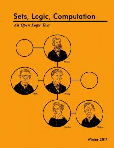
w

Figure 1: The Kripke Model K .

171 The second modification is as follows: we delete certain edges and replace them with back edges (and finally, delete all the states that are reachable from ε). An edge from track ρ to ρ is deleted iff ρ is labeled by cycle and ρ and the initial cycle state of ρ are labeled by the same state of K . In order to illustrate the construction UK , we provide an example in Figure 1 and Figure 2. To make notation easier in the figure, we abbreviate new by n and cycle by c. Also, instead of writing ρ for a state, we only write the pair of labels lst(ρ). The back edges are those that are not straight lines.

Theorem 3. CTL? has a tree-like model property. Every satisfiable formula of CTL? is satisfiable in a tree with back edges. ε

This follows immediately from the following proposition. Proposition 1. Let K = hAP, W, R, L, wI i be a Kripke model, let UK = hAP• , W• , R• , L• , w•I i be its tree-like unwinding. Then the relation {(w• , pr(w• )) : w• ∈ W• } is a cycle-bisimulation. Hence, K and UK satisfy exactly the same formulas in CTL? .

(w, n)

(v, n)

(w, n)

(w, n)

(v, n)

(w, n)

(w, c)

(v, n)

...

(v, n)

(w, n)

(w, c)

Before finishing the section on model properFigure 2: The tree with back edges T (K ). ties, we state one more property concerning the tree-like unwinding of a model. It states that if a formula is true in a tree-like unwinding, then we may assume the “witness” cycles (for the subformulas of the form E s ψ) to be simple cycles (defined below). The property is not that interesting in itself, but it will play an important role in the next section for obtaining a 2E XP T IME upper-bound for the satisfiability problem of the existential fragment of CTL? . Definition 7. A cycle π is a simple cycle if there is a sequence (ni )i∈N such that • ni < ni+1 and πni = π , for all i ∈ N; • for all i ∈ N and for all ni < j < k < ni+1 , we have π j 6= πk . A (state or path) formula ϕ is in normal form if for all subformulas ¬ψ in sub(ϕ), the formula ψ is a variable. Given a formula ϕ in normal form, we define its simple cycle translation as the formula obtained by replacing each symbol E in the formula ϕ, by the symbol E s . The simple cycle translation of ϕ is denoted by (ϕ)s . The semantics of the formulas of the form (ϕ)s is defined by induction on ϕ. The basic and induction cases are defined as in Definition 3, with the additional induction step: K , w |= E s ψ if there is a simple cycle π with beginning state w, such that K , π |= ψ. Proposition 2. Let ϕ be a formula in CTL? in normal form and let K be a Kripke model. Then K |= ϕ iff UK |= (ϕ)s , where UK is the tree with back edges as in Definition 5. Expressiveness We now investigate the expressive power of CTL? w.r.t. the usual temporal logics. All the results are collected in the following theorem. Theorem 4 (Expressiveness comparison). CTL? is strictly more expressive than CTL? and is incomparable with the µ C ALCULUS.

172

Cycle Detection in Computation Tree Logic

Proof. We observed in the proof of Theorem 1 that ϕ1 = AG¬E > is satisfiable but does not admit any finite model. Since CTL? and the µ C ALCULUS have the finite-model property, this implies that ϕ1 is not equivalent to any formula in CTL? or in the µ C ALCULUS. By using the result that there is no LTL formula expressing that a proposition p is true in every even state [28], we can show that the µ C ALCULUS formula ψ = νx.p ∧ 22x is not equivalent to any formula in CTL? . Note that ψ is true in a model if for all paths π starting from the initial state, p is true in every even state (π)2i of the path π.

4

Decision Problems

In this section, we deal with the solution of the model-checking and satisfiability problems for CTL? . Regarding the former, we show that we retain the same complexity as for CTL? , that is PS PACE. Concerning satisfiability, we also retain the same complexity of CTL? if we restrict to the existential-cycle fragment of the logic, that is 2E XP T IME. Conversely, we show that it is 3E XP T IME for the whole logic. Model Checking For the solution of the model-checking problem of CTL? , we employ a standard bottom-up procedure on the nesting of the path quantifiers of the specification under exam, which extends the one originally proposed for CTL? [10]. With more details, starting from the innermost state formulas ϕ of the kind Eψ, Aψ, E ψ, and A ψ, we determine their truth value over a KS K at a world w ∈ W by ϕ checking the emptiness of a suitable nondeterministic B¨uchi word automaton NK ,w . In case of a positive result, we enrich the labeling of the world w with a fresh proposition ϕ representing the formula ϕ itself. Obviously, the path formula ψ is just seen as a classic LTL formula, where all its subformulas of the kind described above are interpreted as atomic propositions whose truth values on the worlds of K are already computed in some previous step of the algorithm. It is important to observe that the difference between the automata for Eψ or Aψ and those for E ψ or A ψ resides in the fact that, for the latter, we have to further verify that the initial state of the path is seen infinitely often. This can be done by means of the standard B¨uchi acceptance condition. Hence, we directly obtain that the model checking for CTL? is not more complex than the same problem for CTL? . Theorem 5. The model-checking problem for CTL? is PS PACE-COMPLETE w.r.t. the formula complexity and NL OG S PACE-COMPLETE w.r.t. the data complexity. Satisfiability Differently from the model checking, the two introduced looping quantifiers E ψ and A ψ heavily affect the satisfiability of CTL? . In particular, since this logic lacks of the standard tree-model property, we cannot use, for the CTL? part of CTL? , the automata approach as proposed in [21]. Instead, we use symmetric two-way alternating tree automata [5], a simplified version of two-way graded alternating parity tree automata [5], which simply extend classic two-way alternating automata over ranked trees [26] to “unranked trees”, i.e., trees with possibly unbounded width. These are automata that allow to traverse a tree in forward and backward. We use these automata here to search for tree representation of the tree-like unwinding of a structure, as described in the previous section. With more details, for every CTL? state formula ϕ, we build an alternating parity two-way tree automaton Aϕ such that a KS K = hAP, W, R, L, wI i is a model of ϕ iff Aϕ accepts a tree TK = hAP ∪ {new, ↑}, W• , R? , L? , w•I i associated with the tree-like unwinding UK =hAP, W• , R• , L• , w•I i of K via the following properties: (i) R? = {(w• , v• ) ∈ R• : |w• | < |v• |}, (ii) L? (w• ) ∩ AP = L• (w• ), (iii) new ∈ L? (w• ) iff lst(w• ) = (w, new), for some w ∈ W, and (iv) ↑ ∈ L? (w• ) iff there exists (w• , v• ) ∈ R• with |v• | < |w• |. Intuitively, TK is built from UK by deleting all back edges (property (i)) and enriching the original labeling of every

G. Fontaine et al.

173

world w• (property (ii)) with new, if the last letter of w• contains the flag with the same name (property (iii)), and with ↑, if w• is the origin of a back edge (property (iv)). It is not hard to see that, for every unwinding UK of a KS K , there exists one and only one tree TK satisfying the previous four properties. Therefore, instead of looking for a model K of ϕ or its tree-like unwinding UK , we just look for its tree representation TK . This idea is at the basis for the automata-theoretic approach described in the proofs of the following theorems. Theorem 6. The satisfiability problem for CTL? can be solved in 3E XP T IME and is 2E XP T IME-HARD. Proof. The 2E XP T IME lower bound for CTL? immediately follows from the one of CTL? . For the 3E XP T IME upper bound, given a CTL? state formula ϕ, we reduce the associated satisfiability question to the emptiness problem of an alternating parity two-way tree automaton Aϕ , whose size and index are, respectively, doubly and single exponential in |ϕ|. For a detailed definition of symmetric alternating parity two-way tree automata and the related concepts of size and index, we refer to [5]. Since the emptiness of Aϕ can be checked in time exponential w.r.t. both its states and index [5], we obtain the desired result 5 . As mentioned above, Aϕ needs to recognize all and only the tree representations TK of the tree-like unwindings UK of KS models K of ϕ. As it is usually done for CTL? , we slightly weaken this property by allowing Aϕ to run on trees that also contain, as labeling of its worlds, the subformulas of ϕ of the form Eψ, Aψ, E ψ, and A ψ, which are interpreted as fresh atomic propositions. We denote by subQ (ϕ) the set of subformulas of ϕ of the form Eψ, Aψ, E ψ, and A ψ. We also let sub¬Q (ϕ) be the the closure under negation of the set subQ (ϕ), i.e., for every Eψ (resp., Aψ, E ψ, A ψ) in sub(ϕ), we have A¬ψ (resp., E¬ψ, A ¬ψ, E ¬ψ) in sub¬ (ϕ). So, instead of considering a model K = hAP, W, R, L, wI i of ϕ, we work on the enriched KS K ? = hAP? , W, R, L? , wI i such that (i) AP? = AP ∪ sub¬ (ϕ), (ii) L? (w) ∩ AP = L(w), and (iii) η ∈ L? (w) iff K , w |= η, for all η ∈ sub¬ (ϕ). set sub(ϕ), i.e., for every Eψ (resp., Aψ, E ψ, A ψ) in sub(ϕ), we have A¬ψ (resp., E¬ψ, A ¬ψ, E ¬ψ) in sub¬ (ϕ). The automaton Aϕ is built as the conjunction of an automaton Aη , for every subformula η ∈ sub¬ (ϕ), and a deterministic safety (i.e., without acceptance condition) automaton Dϕ used to verify that ϕ is satisfied at the root of the input tree TK , when ϕ is interpreted as a Boolean formula on AP? . In addition, Aϕ needs to check that, if a world is not labeled by a state formula η ∈ sub¬ (ϕ), it is necessarily labeled by a formula η ∈ sub¬ (ϕ) equivalent to its negation, i.e., η ≡ ¬η. The automaton Aη is committed to check that a world labeled by η ∈ sub¬ (ϕ) really satisfies this formula. Formally, we have V Aϕ , Dϕ ∧ η∈sub¬ (ϕ) Aη . So, its size is the sum of the sizes of the components. The construction of Dϕ is trivial. Moreover, the automata for Aψ and A ψ can be directly derived from the automaton for E¬ψ and E ¬ψ by replacing ∨ and 3 with ∧ and 2 in their definitions. Hence, we just focus on the constructions for the latter. We start with the construction of AEψ for Eψ. Consider the nondeterministic B¨uchi word automaton ? Nψ =h2AP , Q, δ , QI , Fi obtained by applying the Vardi-Wolper construction to ψ which is read as an LTL formula over AP? [27]. We set as a two-way B¨uchi tree automaton AEψ , hΣ? , Q? , δ ? , q?I , F? i, where the ? alphabet Σ? , 2AP ∪{new,↑} augments the set of extended atomic propositions AP? with the symbols new and ↑, as required by the definition of the tree representations TK . The set of states Q? , {q?I }∪Q×{↓, ↑} contains the initial state q?I plus two copies of the states of Nψ , one for each direction of navigation over the tree TK . For the B¨uchi acceptance condition we consider the set F? , {q?I } ∪ F × {↓}. The definition of the transition function δ ? follows. For the sake of readability, we divide it in three parts, depending on whether it predicates on q?I , a state q flagged with ↓ or a state q flagged with ↑. 5 In

particular, Theorem 6.7 in [5] can be used for the translation. Observe that, since we do not make use of any graded modalities (our box and diamond symbols stand for [[0]] and hh0ii in their syntax) the resulting automaton is simply a symmetric non-deterministic tree automaton.

174

Cycle Detection in Computation Tree Logic • The initial state q?I is used to start the evaluation of the formula Eψ on every world of the input tree labeled by q?I . This is done by starting the simulation of Nψ . Formally, we have that W δ ? (q?I , σ ) , (2, q?I ) ∧ q∈QI (ε, (q, ↓)), if Eψ ∈ σ , and δ ? (q?I , σ ) , (2, q?I ), otherwise. • Every copy of a state q ∈ Q flagged with ↓ is used to effectively verify the existence of an infinite path in UK satisfying ψ. This is done by guessing an extension of the finite path built up to now and sending, to the corresponding direction, a successor p of q that complies with the transition function δ of Nψ , when the labeling σ of the world under exam is read. As the input tree TK is a representation of the tree with back edges UK , we have also to take them into account when we guess the extension of the path from a world labeled with ↑. This is done by sending up along the tree the copy of the state p flagged with ↑, which is used to simulate a jump to the world destination W of the back edge. Formally, we have δ ? ((q, ↓), σ ) , p∈δ (q,σ ∩AP? ) (3, (p, ↓)) ∨ ↑ (p), where ↑ (p) is set to (ε, (p, ↑)) if ↑ ∈ σ , and to f, otherwise. • Finally, for every copy of a state q ∈ Q flagged with ↑, we only have to modify the state and the direction of the automaton when we are approaching to the destination of the back edge that gave rise to the evaluation of (q, ↑). Fortunately, due to the structure of the tree-like unwinding UK and, consequently, of its tree representation TK , when we reach a world labeled by new, we are sure that the immediate ancestor of this world is the destination of the back edge. Thus, we can immediately change the flag of the state q to ↓ in order to resume the verification of the path formula ψ. Formally, δ ? ((q, ↑), σ ) , (↑, (q, ↓)), if new ∈ σ , and δ ? ((q, ↑), σ ) , (↑, (q, ↑)), otherwise.

Now, by construction, it is not hard to prove that AEψ correctly verifies that every world of TK labeled by Eψ satisfies Eψ in UK . Also, by the Vardi-Wolper procedure, it follows that |Q| = O(2|ψ| ). Consequently, the size of AEψ is exponential in the length of Eψ. The construction of AE ψ is quite more complex than the one previously described, as it also requires a projection operation that is the reason behind the exponential gap between the upper and lower bounds. Differently from the automata for classic path quantifiers, we cannot evaluate the correctness of the labeling E ψ on all worlds of the tree in one shot. This is because of the possible interactions among the cycles starting in different worlds, which does not allow us to determine which is the origin of the path we are interested in. Consequently, we have to focus on one world labeled by E ψ at a time and check the existence of a path passing infinitely often through that world, which also satisfies the property ψ. This unique world is identified by a fresh symbol #. Then, an universal projection operation over such a symbol will take care of the fact that this check has to be done for every possible world labeled by E ψ. Formally, AE ψ is built as follows: Π∀# (N# ∨ AE# ψ ). Intuitively, we make a universal projection over # of a disjunction between the automaton N# , accepting all trees where the labeling # is incorrect (i.e., there are more than one occurrences of # or this symbol is on a world that is not labeled by E ψ), and the automaton AE# ψ , verifying the existence of a path satisfying ψ that starts and passes infinitely often through the world labeled by #. The construction of N# is trivial. For the computation of the projection, we use the equality Π∀# A = ¬Π∃# ¬A . Note however that there is no known projection operation that can act directly on a two-way automaton. Instead, we have first to translate it into a nondeterministic one-way automaton [5] and then apply the standard projection. Due to the nondeterminization procedure, Π∀# A has exponential size w.r.t. that of A . So, AE ψ is exponential in the size of AE# ψ . ?

It remains to define the latter automaton. As above, let Nψ =h2AP , Q, δ , QI , Fi be the nondeterministic B¨uchi word automaton obtained by applying the Vardi-Wolper construction to ψ. Then, we set AE# ψ , ? hΣ? , Q? , δ ? , q?I , F? i as a two-way B¨uchi tree automaton having alphabet Σ? , 2AP ∪{new,↑,#} . The set of states Q? , {q?I } ∪ Q × {f, t} × {#, ↓, ↑} contains the initial state q?I plus six copies of the states of Nψ .

G. Fontaine et al.

175

Each of them is flagged with a Boolean value keeping track of the original acceptance condition derived from Nψ and a symbol indicating the direction of navigation over the tree. Differently from the previous case, we have also # as a flag in order to indicate the passage though the state labeled by the flag itself. For the B¨uchi acceptance condition we consider the set F? , {q?I } ∪ Q × {t} × {#}. Intuitively, apart from the initial state, we assume as final those states that certify both the passage through the origin of the path indicated by # and the possibly previous occurrence of an accepting state. It remains to define the transition function δ ? . Here we use α(q, α) to denote the Boolean value t, if q ∈ F, and α, otherwise. • The initial state q?I is used to start evaluating the formula E ψ on the unique world of the input tree W labeled by #. Formally, we have δ ? (q?I , σ ) , q∈QI (ε, (q, α(q, f), ↓)), if # ∈ σ , and δ ? (q?I , σ ) , (2, q?I ), otherwise. Note that, since we are just starting with the simulation of Nψ , the flag α(q, f) concerning the memory on the acceptance condition only depends on the state q, as the second argument is fixed to f. • Since a state (q, α, #) is simply used to verify the passage through the starting point of the path satisfying ψ, the automaton has to reset the memory on the acceptance condition and continue with the simulation of Nψ . Formally, δ ? ((q, α, #), σ ) , (ε, (q, f, ↓)). • The automaton AE# ψ on the state (q, α, ↓) behaves similar to AEψ on (q, ↓). One difference resides in the update α(p, α) of the memory on the acceptance condition, which takes into account both the previous memory α and the membership of p in F. The other difference is that, if σ contains the symbol #, we have to record this fact in the state, by swapping the flag from ↓ to #. Formally, W we have δ ? ((q, α, ↓), σ ) , p∈δ (q,σ ∩AP? ) (3, (p, α(p, α), β )) ∨ ↑ (p), where β = #, if # ∈ σ , and β = ↓, otherwise; moreover, ↑ (p) is set to (ε, (p, α(p, α), ↑)) if ↑ ∈ σ , and to f, otherwise. • Finally, as for AEψ , a state of the form (q, α, ↑) identifies the destination of a back edge. Thus, we have δ ? ((q, α, ↑), σ ) , (↑, (q, α, ↓)), if new ∈ σ , and δ ? ((q, α, ↑), σ ) , (↑, (q, α, ↑)), otherwise. Finally, the size of AE# ψ is exponential in the length of E ψ, which implies that AE ψ is doubly exponential w.r.t. the same length. In case we want to restrict our attention to the satisfiability of the CTL? fragment having only existential looping quantifiers, we can improve the previous proof, obtaining a tight 2E XP T IME procedure, by providing a single exponential construction for the automaton AE ψ . Indeed, thanks to the simple cycle property of the verification of the formula E ψ on the tree-like unwinding UK , we can just focus on cycle paths of UK going through the successors of their origin labeled by new. In this way, there are no interactions among the paths that start at different worlds labeled by E ψ, since two paths passing through the same world necessarily use different successors. Consequently, we can always uniquely identify the origin of a path on which we have to pass infinitely often. Unfortunately, the same idea cannot be exploited for the verification of the universal looping quantifiers A ψ, as we have to check the property ψ on all cycle paths and not only on those that are simple. At the moment, it is left open whether a 2E XP T IME satisfiability procedure for the whole CTL? logic exists. Theorem 7. The satisfiability problem for the existential-cycle fragment of CTL? is 2E XP T IME-COMPLETE.

5

Discussion

To conclude, we give a concise overview of the main properties of the cycle-logic extension we have introduced. We also explain why this extension is natural and why, given our results, we have decided to focus our presentation on the cycle-logic CTL? .

176

Cycle Detection in Computation Tree Logic

CTL? allows us to quantify only over cycles, that is, paths such that the initial state occurs infinitely often. Hence, it has been natural to consider also a more general logic (denoted by ECTL? ) allowing us to test whether any arbitrary state of a given path occurs infinitely often in the path. More formally, ECTL? is the extension of CTL? obtained by adding the symbol . This symbol is treated as an atomic path formula and is true at a state in a path iff the state occurs infinitely often in the path. It is easy to see that ECTL? is an extension of CTL? . We have studied several properties about ECTL? and, among the others, we have shown that this logic does not preserve the cycle-bisimulation property. Clearly, one can use a stronger notion of bisimulation under which ECTL? can still retain the invariance. However, we came up with notions that are not very intuitive (as the notion of cycle-bisimulation) and not useful to prove any kind of tree-like model property. Given these negative results, we decided to not present extensively this part. We would like to mention that we also considered the extension of LTL with the symbol . It is not hard to show that it is a proper extension of LTL and is orthogonal to ω-regular expressions. We can also prove that the finite satisfiability problem for that logic is decidable (using an adaption of the proof for LTL [27]). We did not present these results by lack of space. Finally, as future work we would like to investigate the use of the introduced cycle construct in the realm of logics for multi-agent systems such as ATL? [2] and Strategy Logic [23]. These logics have been proved to be useful to reasoning about strategic abilities in a number of complicated settings. In particular, the latter is able to express sophisticated solution concepts such as Nash Equilibria and Subgame Perfect Equilibria, as well as they it has been used to express iterative extensive game forms such as the iterated prisoner dilemma. In all these contexts, talking explicitly about cycles could play a central role in solving the related game questions.

Acknoledgments Aniello Murano and Loredana Sorrentino are partially supported by the GNCS 2016 project: Logica, Automi e Giochi per Sistemi Auto-adattivi. Giuseppe Perelli thanks the support of the ERC Advanced Grant 291528 (“Race”) at Oxford.

References [1] R. Alur & T.A. Henzinger (1998): doi:10.1145/295656.295659.

Finitary Fairness.

TOPLAS 20(6), pp. 1171–1194,

[2] R. Alur, T.A. Henzinger & O. Kupferman (2002): Alternating-Time Temporal Logic. JACM 49(5), pp. 672–713, doi:10.1145/585265.585270. [3] R. Alur & S. La Torre (2004): Deterministic generators and games for LTL fragments. ACM Transactions on Computational Logic (TOCL) 5(1), pp. 1–25, doi:10.1145/963927.963928. [4] B. Aminof, A. Murano, S. Rubin & F. Zuleger (2016): Prompt Alternating-Time Epistemic Logics. In: KR’16, AAAI Press, pp. 258–267. [5] P.A. Bonatti, C. Lutz, A. Murano & M.Y. Vardi (2008): The Complexity of Enriched muCalculi. LMCS 4(3), pp. 1–27, doi:10.2168/LMCS-4(3:11)2008. [6] L. Bozzelli, A. Murano & A. Peron (2010): Pushdown Module Checking. FMSD 36(1), pp. 65–95, doi:10.1007/s10703-010-0093-x. [7] K. Chatterjee, T.A. Henzinger & F. Horn (2010): Finitary Winning in omega-Regular Games. TOCL 11(1), pp. 1:1–26, doi:10.1145/1614431.1614432.

G. Fontaine et al.

177

[8] E.M. Clarke & E.A. Emerson (1981): Design and Synthesis of Synchronization Skeletons Using BranchingTime Temporal Logic. In: LP’81, LNCS 131, Springer, pp. 52–71, doi:10.1007/BFb0025774. [9] E.M. Clarke, E.A. Emerson & A.P. Sistla (1986): Automatic Verification of Finite-State Concurrent Systems Using Temporal Logic Specifications. TOPLAS 8(2), pp. 244–263, doi:10.1145/5397.5399. [10] E.M. Clarke, O. Grumberg & D.A. Peled (2002): Model Checking. MIT Press. [11] E.A. Emerson & J.Y. Halpern (1985): Decision Procedures and Expressiveness in the Temporal Logic of Branching Time. JCSS 30(1), pp. 1–24, doi:10.1016/0022-0000(85)90001-7. [12] E.A. Emerson & J.Y. Halpern (1986): “Sometimes” and “Not Never” Revisited: On Branching Versus Linear Time. JACM 33(1), pp. 151–178, doi:10.1145/4904.4999. [13] E.A. Emerson & C.S. Jutla (1988): The Complexity of Tree Automata and Logics of Programs (Extended Abstract). In: FOCS’88, IEEE Computer Society, pp. 328–337, doi:10.1109/SFCS.1988.21949. [14] A. Ferrante, A. Murano & M. Parente (2008): Enriched Mu-Calculi Module Checking. LMCS 4(3), pp. 1–21, doi:10.2168/LMCS-4(3:1)2008. [15] E. Gr¨adel, W. Thomas & T. Wilke (2002): Automata, Logics, and Infinite Games: A Guide to Current Research. LNCS 2500, Springer, doi:10.1007/3-540-36387-4. [16] S.A. Kripke (1963): Semantical Considerations on Modal Logic. doi:10.1002/malq.19630090502.

APF 16, pp. 83–94,

[17] O. Kupferman, G. Morgenstern & A. Murano (2006): Typeness for omega-Regular Automata. IJFCS 17(4), pp. 869–884, doi:10.1142/S0129054106004157. [18] O. Kupferman, N. Piterman & M.Y. Vardi (2002): Pushdown Specifications. In: LPAR’02, LNCS 2514, Springer, pp. 262–277, doi:10.1007/3-540-36078-6 18. [19] O. Kupferman, N. Piterman & M.Y. Vardi (2009): From Liveness to Promptness. FMSD 34(2), pp. 83–103, doi:10.1007/s10703-009-0067-z. [20] O. Kupferman, A. Pnueli & M.Y. Vardi (2012): Once and For All. doi:10.1016/j.jcss.2011.08.006.

JCSS 78(3), pp. 981–996,

[21] O. Kupferman, M.Y. Vardi & P. Wolper (2000): An Automata Theoretic Approach to Branching-Time Model Checking. JACM 47(2), pp. 312–360, doi:10.1145/333979.333987. [22] O. Kupferman, M.Y. Vardi & P. Wolper (2001): doi:10.1006/inco.2000.2893.

Module Checking.

IC 164(2), pp. 322–344,

[23] F. Mogavero, A. Murano, G. Perelli & M.Y. Vardi (2014): Reasoning About Strategies: On the Model-Checking Problem. TOCL 15(4), pp. 34:1–42, doi:10.1145/2631917. [24] F. Mogavero, A. Murano & L. Sorrentino (2015): On Promptness in Parity Games. Fundamenta Informaticae 139(3), pp. 277–305, doi:10.3233/FI-2015-1235. [25] A. Pnueli (1977): The Temporal Logic of Programs. In: FOCS’77, IEEE Computer Society, pp. 46–57, doi:10.1109/SFCS.1977.32. [26] M.Y. Vardi (1998): Reasoning about The Past with Two-Way Automata. In: ICALP’98, LNCS 1443, Springer, pp. 628–641, doi:10.1007/BFb0055090. [27] M.Y. Vardi & P. Wolper (1986): An Automata-Theoretic Approach to Automatic Program Verification. In: LICS’86, IEEE Computer Society, pp. 332–344. [28] P. Wolper (1983): Temporal Logic Can Be More Expressive. IC 56(1-2), pp. 72–99, doi:10.1016/S00199958(83)80051-5. [29] W. Zielonka (1998): Infinite Games on Finitely Coloured Graphs with Applications to Automata on Infinite Trees. TCS 200(1-2), pp. 135–183, doi:10.1016/S0304-3975(98)00009-7.