D-Swoosh: A Family of Algorithms for Generic, Distributed Entity ...

D-Swoosh: A Family of Algorithms for Generic, Distributed Entity Resolution Omar Benjelloun Tait E. Larson

Hector Garcia-Molina David Menestrina

Heng Gong Hideki Kawai Sutthipong Thavisomboon

Stanford University {benjello,hector,henggong,hkawai,telarson,dmenest,sthavis}@cs.stanford.edu

Abstract

ER is a critical component of any information integration task, whether we are looking for terrorist activities, combining customer records after two companies merge, or consolidating student records for students that change schools. Unfortunately, ER is usually a computationally expensive process. First, there are often many records. In a comparison shopping application, for instance, tens of millions of records can be received daily from different merchants. Second, the record comparisons that are performed are typically expensive, as compared to, say, checking an equality predicate in a database join. For example, to compare records, we may perform maximal common sub-sequence computations on text fields. We may also look up values in large dictionaries of canonical terms (e.g., to map “Bobby” to “Robert”). We may also need to do language or character set translations on some fields.

Entity Resolution (ER) matches and merges records that refer to the same real-world entities, and is typically a compute-intensive process due to complex matching functions and high data volumes. We present a family of algorithms, D-Swoosh, for distributing the ER workload across multiple processors. The algorithms use generic match and merge functions, and ensure that new merged records are distributed to processors that may have matching records. We perform a detailed performance evaluation on a testbed of 15 processors, for cases where application knowledge can eliminate some comparisons and where all records must be matched. Our experiments use actual comparison shopping data provided by Yahoo!. (keywords: Entity Resolution, Information Integration, Data Cleaning)

There are generally two ways to deal with the extremely high computational load of ER: One is to “partition” the problem using semantic knowledge and the other is to exploit multiple processors. As an example of partitioning, we can divide our product records (in the comparison shopping application) by category (CDs, MP3 players, cameras, etc.), and then only try to match records in the same category (possibly with some overlap between partitions, e.g., if products have multiple categories). Here we are using the knowledge that records in different categories will never match. Of course, in some applications we may not have such knowledge, or we may not be willing to assume that the categorization is perfect. But even with semantic knowledge, there may still be many comparisons to perform because the resulting categories or buckets are still relatively large. Thus, we believe that the second option, parallelism, will be essential in many applications. In this paper we focus on techniques for distributing the ER process over multiple processors, both

1 Introduction The process of Entity Resolution (ER) identifies records that refer to the same real-world entity and merges them. For example, in a comparison shopping application, records arrive from different stores. Two records r1 and r2 may refer to exactly the same product, e.g., an iPod, but may not have a unique identifier that links them. (For instance, each store may use a different identification scheme, and in addition, product names, descriptions and other fields may contain typos or may be missing.) If r1 and r2 match, i.e., are deemed to be “similar enough” that they represent the same product, then it may be useful to merge them into, say, r12 , a “composite” of the original records. Because r12 contains more information that r1 or r2 alone, it may now match other records that neither r1 nor r2 match. 1

for the case where we have no semantic knowledge, and the case where we have ways of partitioning the problem. A majority of the work on ER to date has been done in the context of a specific application, e.g., resolving author or customer records. Thus, it is often hard to generalize the results, i.e., it is difficult to separate the applicationspecific techniques from the ideas that could be used in other contexts. To clearly separate the application details from the generic ER processing, in this paper we encapsulate the record matching and merging into two black-box functions. The match function takes as input two records, and decides if they represent the same real-world entity. The match function may compute similarities between the two records (and perhaps other records), but eventually it must decide if the two records should be merged. If records are to be combined, the merge function is called to generate a new composite record. Note that by encapsulating match and merge, we are separating accuracy issues from performance issues. From our perspective, accuracy (i.e., if the composite records are “correct”) is a function of the match and merge functions, which we are given. Our job is only to invoke these functions as few times as necessary, and to distribute the work of evaluating the functions across processors.

The matches in our example could have been found in a different order, e.g., perhaps r0 and r4 are merged first, and then with r3 . In this paper we will assume that the order of merging does not impact the final outcome, and that the records that went into a composite record can be deleted from the final answer. (The precise properties are given in Section 2.) However, it is important to note that if these properties do not hold, our distributed algorithms can be extended in a straightforward way (for example, we would not delete records after they merge). Say we want to distribute this ER processing over three processors, P0 , P1 and P2 . The problem is analogous to performing a distributed self-join in a database system: we wish to distribute the records to the processors so that the comparisons are done in parallel. However, there are two important differences with joins: • With a join, the match function is simple and known, so we can exploit this knowledge. For example, if the common join attribute is X, we can distribute records with X < 10 to one processor, those with X ≥ 10 to another, and comparisons will be localized to one processor. With ER, we may not know anything about the match function, so we need to develop mechanisms that work in general. • With ER, unlike joins, there is a “feedback” loop where merged records need to be re-distributed and compared to other records.

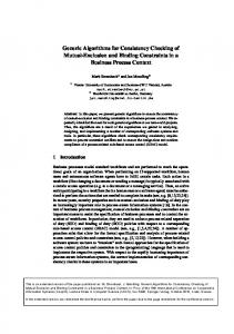
1.1 Overview of Our Approach To motivate our approach, and to illustrate some of the challenges faced, consider the following simple example. Say we have 6 input records, r0 through r5 . Figure 1 shows one possible ER outcome for this example, assuming we run on a single processor. After comparing the input records, we discover that r0 and r3 match, so they are merged into r6 . The new record then matches with r4 ; the resulting merged record is r8 . In this example, r2 and r5 also merge, into record r7 . The final answer is {r1 , r7 , r8 }, where none of these records match any further.

To address theses issues, we use a general distribution function we call scope. That is, scope(ri ) gives us the set of processors where ri will be sent. For example, Figure 2 shows one possible scope function. Note that this scope function can be expressed by scope(ri ) = {Pj , Pk } where j = i mod 3, and k = (i + 1) mod 3. P0 r0 r2 r3 r5 r6 r8

P1 r0 r1 r3 r4 r6 r7

P2 r1 r2 r4 r5 r7 r8

Figure 2: One possible scope function Notice that for every pair of records, there is at least one processor that has both records. For example, the pair r0 , r2 is at P0 , and the pair r0 , r3 is at P0 and P1 . Thus, if

Figure 1: A sample run of Entity Resolution 2

each processor executes all match comparisons on records in its scope, we will not miss any comparisons. Our algorithm will proceed by distributing the input records to processors using the scope function. Then each processor will apply the match function to the pairs of records it has.

parisons, analogous to what is done with joins. For instance, if product records can only match if their “price” attribute is numerically close, we can design a scope function that assigns records to processors by price, so a processor only gets records whose price is close. We discuss Of course, with this scheme we may perform redun- scope and resp functions that exploit semantic knowledge dant comparisons, e.g., in our case, the r0 , r3 comparisons in Section 4.2. would be performed by both P0 and P1 . To avoid redun- In summary, the contributions we make are: dant comparisons we also introduce a responsible func• We define the problem of distributed entity resolution (denoted resp): processor Pk will apply the match tion, for the case where black-box match and merge function to ri and rj only if it is in the scope of both functions are used (Section 3). records, and resp(Pk , ri , rj ) is true. Intuitively, the re• We present a generic, distributed algorithm, Dsponsible function needs to compute the set of processors Swoosh, that runs ER on multiple processors using that will have both ri and rj , and then deterministically scope and responsible functions, and computes the choose one of them, without overloading some procescorrect answer (Section 3.2). sors. Since the responsible function typically performs simple arithmetic (or more basic) operations, it is much • We suggest a variety of scope and responsible funccheaper to compute than the match function, and hence tions, some for scenarios with no semantic knowlthe saving can be significant. In Sections 4.1 and 4.2, we edge, others that exploit knowledge that often arises provide several instances of scope and resp functions. in ER applications (Section 4). When a processor finds a match among its records, it • We present metrics to evaluate distributed ER, and computes the merged record and distributes it so that the conduct a detailed evaluation of D-Swoosh and the new record is compared against all existing records. Thus, various scope and responsibility functions on a 15 scope and responsible functions should work with merged processor testbed, using comparison shopping data records, and guarantee that no matches are missed. Howprovided by Yahoo! (Section 5. Our results show ever, even with a good responsible function, it will be that the ER process can take advantage of parallelism impossible to avoid all redundant work due to the conwith great benefit. current execution of related comparisons. To illustrate this unavoidable redundancy, suppose that three records Background material is given in Section 2, and related ri , rj and rk all match pairwise. Say that processor P0 work is presented in Section 7. Section 8 is our concluis responsible for the ri , rj comparison, processor P1 for sion. the ri , rk pair, and P2 for the rj , rk pair. Each processor in parallel will discover a match and will merge its pair of records. The three resulting records, rij , rik and 2 Preliminaries rjk are distributed, and compared again, and each pair of the new records could be the responsibility of a differ- We first define our generic setting for ER; additional deent processor. Each of these processors will then inde- tails can be found in [2]. We are given a set of records pendently compute the same merged record rijk (recall R = {r1 , . . . , rn } to be resolved. The match function that merge order is not important). Thus, rijk is gener- M (ri , rj ) evaluates to true if records ri and rj are deemed ated three times. Our algorithm will eventually remove to represent the same real-world entity. As shorthand we the duplicate copies, but we have performed more work write ri ≈ rj . If ri ≈ rj , a merge function generates than necessary to get rijk . Depending on the timing of hri , rj i, the composite of ri and rj . events, some of the redundant work may be avoided, but Match and merge functions are usually not arbitrary, there is always the potential for redundancy. As a mat- and may satisfy the following four simple properties: ter of fact, adding processors beyond some limit may be counter productive, as it may lead to more redundant work • Commutativity: ∀r1 , r2 , r1 ≈ r2 iff r2 ≈ r1 , and if and more communication overhead. One of our goals here r1 ≈ r2 , then hr1 , r2 i = hr2 , r1 i. is to empirically study these issues, and to evaluate how • Reflexivity/Idempotence: ∀r, r ≈ r and hr, ri = r. much redundant work may be done in practice. • Merge representativity: If r3 = hr1 , r2 i then for any r4 s.t. r1 ≈ r4 , we also have r3 ≈ r4 .

If we have semantic knowledge, we may develop scope and responsible functions that reduce the number of com3

• Merge associativity: ∀r1 , r2 , r3 such that both back into the input set R, and deletes the pair of matching hr1 , hr2 , r3 ii and hhr1 , r2 i, r3 i exist, hr1 , hr2 , r3 ii = records immediately. hhr1 , r2 i, r3 i. To illustrate the operation of R-Swoosh, consider a run on the instance of our initial example, supposing the As discussed in [2], if these properties do not hold, the records are processed in the order of their identifiers. We entity resolution problem becomes much more expensive. take r0 and compare it against records in R′ . Since R′ For instance, without associativity we must consider all is initially empty, there are no matches with r0 , so r0 possible orders in which records may match and merge. is moved to R′ . Next, r1 is compared against records In a sense the solution will not be “consistent” because in R′ , i.e., against r0 . In our example (Figure 1), there there can be multiple composite records that can be de- are no matches, so r1 is also moved to R′ . Record r2 is rived from the same matching records. Because of these moved to R′ in a similar fashion. When r3 is compared problems, there is a strong incentive for programmers to against R′ , we discover that r0 and r3 match. Theredesign match and merge functions that satisfy the above fore, r6 = hr0 , r3 i is added to R, and r0 and r3 are properties. Thus, in this paper we focus on applications removed from R′ and R, respectively. Next, r4 is prowhere these properties hold. However, as noted earlier, cessed and added to R′ , r5 is processed generating r7 = the algorithms we present can be extended to perform the hr2 , r5 i, which is added into R; r6 is processed generadditional comparisons required if the properties do not ating r8 = hr4 , r6 i into R. The remaining R records hold. are processed and moved to R′ . At the end, R′ holds During entity resolution, we may generate merged ER(R) = {r1 , r7 , r8 }. records that do not carry additional information, relative In [2], we also give a variant of the algorithm, Fto other records. For instance, say records ri , rj , rk have Swoosh, that efficiently caches the results of value commerged into record rijk (via two merges). In this case parisons. we no longer need records ri , rij , or any other records derived from a subset of {ri , rj , rk }. We call the unnecessary records dominated. 3 Distributed ER Definition 2.1 Given two records, r1 and r2 , we say that In this section, we extend the R-Swoosh sequential algor1 is dominated by r2 , denoted r1 ≤ r2 if hr1 , r2 i = r2 . rithm for generic ER to be distributed, in order to run in parallel on multiple processors. We start by defining the One can easily verify that domination is a partial order primitives needed to capture distribution, then present the on records. We are now ready to define the entity resolualgorithm. tion problem: Definition 2.2 Given a set of input records R, an Entity 3.1 Distribution Primitives Resolution of R, denoted ER(R) is a set of records such Our p processors are P = {P0 , . . . , Pp−1 }. As mentioned that: in the introduction, we introduce a “scope” function to • Any record in ER(R) is derived (through merges) distribute records across processors and a “responsible” from records in R; predicate to reduce redundant work, by deciding which processors are responsible for which comparisons. These • Any record that can be derived from R is either in are defined formally as follows. ER(R), or is dominated by a record in ER(R); Definition 3.1 A scope function is a function from R, the domain of records to 2P that assigns to each record r a subset scope(r) of the processors. A responsible predicate is a Boolean predicate over P × R × R. When resp(Pi , r, r′ ) = true, we say that processor Pi is responsible for the pair of records (r, r′ ). Scope and resp satisfy the following “coverage” property. Coverage property: For any pair of matching records r, r′ , there exists at least one processor Pi such that Pi ∈ scope(r) ∩ scope(r′ ) and resp(Pi , r, r′ ) = true.

• No two records in ER(R) match, and no record in ER(R) is dominated by any other. In [2], we show that the entity resolution of R is unique, and provide R-Swoosh, an optimal algorithm for performing entity resolution on a single processor. R-Swoosh incrementally processes the input records, while maintaining a set R′ of (so far) non-dominated, non-matching records. R-Swoosh performs a merge as soon as a pair of matching records is found, puts the obtained record 4

ure 2) assigns to P0 records {r0 , r2 , r3 , r5 }, while P1 gets {r0 , r1 , r3 , r4 } and P2 gets {r1 , r2 , r4 , r5 }. Let us focus on the actions at P0 . Say P0 is responsible for the r0 , r3 comparison, but not the r2 , r5 one. When P0 merges r0 , r3 into r6 , it sends −(r0 ), −(r3 ) messages to itself and P1 (the processors that have these records in their scope). It also sends +(r6 ) to the processors in scope(r6 ), i.e., P0 and P1 . In the meantime, P0 will be getting messages from other processors. For example, the processor responsible for the pair r2 , r5 will send to P0 messages −(r2 ), −(r5 ) when those records merge. As the messages arrive at P0 , they are processed. For instance, when the −(r2 ) message arrives at P0 , record r2 is removed from R0′ , if it is there. 3.1.1 Distributed Computing Model Note that r2 may not be in R0′ , e.g., the initial +(r2 ) mesWe make the standard assumptions about our distributed sage may not have arrived. This is why the −(r2 ) message computing model: First, we assume that no messages ex- is “remembered” in the set D0 : when r2 finally arrives, it changed between processors are lost. Second, that mes- will be ignored because r2 is in D0 . Records r6 and r4 sages sent from a processor to another are received in the will be merged at processor P1 to form r8 , +(r8 ) will be same order as they are sent, and processed in that same sent to processors r0 and r2 . order (this can be achieved easily by numbering the messages). Finally, that processors are able to use some exist- Theorem 3.2 Given a set of records R, the D-Swoosh aling distributed termination detection technique to detect gorithm terminates and computes ER(R). that they are all in an idle state (see, e.g., [6]). Proof In [2], we show that given a set of records R, ER(R) can be computed by any maximal derivation se3.2 The D-Swoosh Algorithm quence of R. A derivation sequence is a sequence of We are now ready to give our general algorithm for dis- merge steps (addition of a merged record) and purge steps tributed ER. The algorithm of Figure 1 asynchronously (deletion of a dominated record). A derivation sequence runs a variant of the R-Swoosh algorithm at each pro- is maximal if no additional merge or purge steps can be cessor Pi . Initially, each Pi receives the records in its performed. To prove the correctness of D-Swoosh, we show that it scope. Each Pi maintains a set Ri′ of non-dominated, nonmatching records. The processor also keeps a set Di of the computes S a maximal derivation sequence of the set I = W ∪ Pi Ri′ , where W is the set of all records pending records it knows have been deleted. When a new (added) record r is received by Pi , it is suc- processing at any of the processors. Since I is initially cessively compared to every record r′ in Ri′ , provided Pi equal to R and W = ∅ when the algorithm terminates, this is responsible for that comparison. If a match is found, the will effectively establish the correctness of D-Swoosh. We first prove that each event handled by a processor matching records are merged immediately, and messages are sent to the relevant processors (identified through the corresponds either to a merge or a purge step on I, or scope function) instructing them to add or delete records. keeps I unchanged. We then prove that the derivation sequence is maximal, and that the algorithm terminates. If no match is found, then r is added to Ri′ . When processor Pi handles a +(r) message, r is either Note that if the new merged record hr, r′ i is identical to either r or r′ , then not all the messages are sent out. Fur- added to Ri′ or a −(r) message is sent to one or more thermore, if hr, r′ i is equal to r, the record we are process- processors. In both cases, r remains in I. If r matches a ing, we continue processing r. If no match is found with record r′ in Ri′ , the two records are merged into r′′ , and any of the Ri′ records, r is added to Ri′ . The algorithm ter- +(r′′ ) is sent to one or more processors (hence added to minates when all processors have resolved all the records W ). In case r′′ was not present in I before (e.g., at some in their scope, and the messages they sent have been re- other processor), the algorithm has performed a merge ceived and processed. The final answer is the union of the step: a record obtained by merging two records previously present in I is added to I. Ri′ sets at the processors. Consider running D-Swoosh on our 6 record example When processor Pi handles a −(r) message, r is redataset. Recall that our example scope function (Fig- moved from Ri′ , hence r is removed from I if no other Interestingly, the coverage property is related to the distributed mutual exclusion problem [8]. We can think of record r as a process that “locks” the processors in its scope. Since r′ also locks its scope, and since scope(r) ∩ scope(r′ ) is not empty, then r and r′ are mutually excluded. Thus, requiring scopes to intersect (so every pair of matching records is compared) is equivalent to requiring the locks to conflict at least one processor. Any coterie [11] used for mutual exclusion can hence be used for guaranteeing coverage in our context. However, we only want coteries that distribute the workload evenly, since we are doing expensive record comparisons and not locking.

5

processor still has r or is waiting to process r. It is easy to see that −(r) messages are only sent when r is known to be dominated by another record in I. Therefore, if r is effectively removed from I, the algorithm has performed a purge step.

3.2.1 Lineage Optimization The algorithm presented above can be improved by considering the lineage of records, i.e., their derivation history. The properties of the match and merge functions entail that some pairs of records can be determined to match without even comparing them, just by looking at the sets of records they were respectively derived from. More precisely, let the base of r, be the set of original records r was derived from. base(r) = {r} for input records, and if r = hr1 , r2 i, then base(r) = base(r1 ) ∪ base(r2 ). The following properties can be shown to hold:

D-Swoosh performs a sequence of merge and purge steps on I, and therefore computes a correct derivation sequence of I. We must now show that the derivation sequence is maximal, i.e., once I stops evolving, no further merge or purge step is possible. We will then show that the algorithm terminates. Observe that for any record r, all messages relevant to r (+(r) or −(r)) are sent exactly to the set of processors in scope(r). Therefore the only processors to ever manipulate r are precisely those in scope(r).

• If base(r1 ) ⊆ base(r2 ) then r1 ≤ r2 (in particular, two records with the same base are identical). • If base(r1 ) ∩ base(r2 ) 6= ∅ then r1 ≈ r2 .

Suppose I does not evolve anymore, and a merge step is still possible, say between records r1 and r2 . W.l.o.g. we can assume that r1 and r2 are not dominated by any other records in I. Therefore a +(r1 ) (resp. +(r2 )) message is received at some point by all the processors in scope(r1 ) (resp. scope(r2 )). By the coverage property, one of the processors in the intersection of these scopes (say, Pi ) is responsible for the pair (r1 , r2 ). Upon receiving the first of these two records (say, r1 ), Pi adds r1 to Ri , because it is not dominated. When Pi receives r2 , it compares it with r1 and performs the merge step, a contradiction.

The first property means that if a record r1 was derived from a subset of the records a record r2 was derived from, then r1 is dominated by r2 . The second property says that if r1 and r2 have some base records in common, then they are known to match and can be merged right away. The D-Swoosh algorithm does not even need to be modified to leverage this lineage information. In fact, for each record r, base(r) can be kept as an extra attribute. The match function can be replaced by a new match function that first checks for a non-empty intersection on the bases of records, and only if the intersection is empty evalSuppose now that I does not evolve, but a purge step is uates the original match function. Similarly, the merge possible, say record r1 is dominated by record r2 . Again, function can be extended to check for an inclusion relaby the coverage property r1 and r2 are handled by at least tionship (and return the non-dominated record immedione processor Pi . Processor Pi must send −(r1 ) to all ately) and to construct the base of merged records. processors in scope(r1 ). After all processors have handled this message, r1 is not in W . Moreover, r1 is not present in any of the Ri′ sets, and cannot reappear because 4 Choosing scope and resp it was added to the Di sets. Therefore, the purge step would effectively have been performed, again a contra- We now consider particular scope and resp functions to diction. distribute the ER work among a set of processors. We start No merge or purge step is possible on the final state of with strategies that are always applicable because they do I, hence the algorithm computes a maximal derivation se- not make any extra assumptions, then turn to strategies quence. We now show that the algorithm terminates. Ob- which exploit existing semantic knowledge. serve that after the algorithm has computed the maximal derivation sequence, no two records may match. Indeed, if two records match, then a merge or purge step would necessarily follow, a contradiction. As a consequence, no more “send” messages are exchanged by processors. Any record in W disappears from there once it has been processed by all the processors in its scope. W eventually becomes empty, and all processors become idle, hence the algorithm terminates.

4.1 Strategies Without Domain Knowledge In this section, we consider strategies in which we do not have any a priori domain knowledge about records, and therefore must consider all possible matches between records. Our goal will be to distribute the work evenly across processors, while trying to reduce communications and redundant computations. We present three schemes: full replication, majority (which generalizes our initial example) and grid. We do not prove it here, but it is not 6

difficult to see that the scope and resp functions given in Tables 1, 2, and 3 satisfy the coverage property of Definition 3.1.

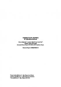
As shown in Table 2, there are three cases to consider in determining where the scopes of two records intersect. For instance, consider two records in buckets b1 and b3 respectively. This situation corresponds to the first case since x − y (i.e., the difference in bucket indexes) is 3 − 1, 4.1.1 Full Replication Scheme which is less than half the processors. Here, the scopes In the full replications scheme, records are sent to all overlap at m = 2 processors: P3 and P4 . The resp funcp processors. The scheme is defined is Table 1, using tion then uses the smallest record identifier to select one the same style that will be used for the other schemes. of these two processors. To select the processor that is responsible for comparing records ri and rj , we select the smallest of the two indexes, i or j, and use it to identify the processor. If records 4.1.3 Grid Scheme identifiers are evenly distributed, this scheme ensures that With the grid scheme (Table 3), we again divide records each processor has a similar number of pairs to compare. into B disjoint buckets. For this scheme, we require that The full replication scheme clearly has a high storage the number of processors be B(B + 1)/2, which correoverhead, so our next two schemes will reduce storage sponds to the number of elements in half a matrix of size costs. However, as shown by our experiments (Section 5), B, including the diagonal. For B = 7 buckets, we need 28 full replication has benefits under some of the other met- processors, which are arranged as illustrated in Figure 4. rics we consider. 4.1.2 Majority Scheme

b0 b1 b2 b3 b4 b5 b6

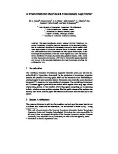
The majority scheme (Table 2) generalizes the scope and resp functions we used in the introduction, from 3 to an arbitrary number p of processors. The essential idea is that if any record has a scope that consists of more than half (i.e., a majority) of the processors, then any pair of records will share at least one common processor in their scopes. We also generalize the resp function such that any pair of record is the responsibility of exactly one processor. With the majority scheme, every processor receives and stores about half of the records in the dataset. P0 b0

b4 b5 b6

P1 b0 b1

b5 b6

P2 b0 b1 b2

b6

P3 b0 b1 b2 b3

P4 b1 b2 b3 b4

P5

b2 b3 b4 b5

b0 P0 P1 P2 P3 P4 P5 P6

b1

b2

b3

b4

b5

b6

P7 P8 P9 P10 P11 P12

P13 P14 P15 P16 P17

P18 P19 P20 P21

P22 P23 P24

P25 P26

P27

Figure 4: Processor arrangement in the grid scheme For the scope, every record in bucket j is sent to the processors that appear on the j th line and column of the (half) matrix. For instance, in our example, records in bucket 3 are sent to processors {P3 , P9 , P14 , P18 , P19 , P20 , P21 }. Observe that processors on the diagonal get records from exactly one bucket, while processors in other positions receive records from two buckets. For the resp function, the processor at the intersection of the ith and j th column is responsible for the pairs of records r, r′ such that one of them is in bucket i and the other in bucket j. Hence, processors on the diagonal are responsible for comparing all the records in their scope, while other processors are only responsible for the pairs of records in their scope which belong to different buckets. To illustrate, in our example, processor P18 has all the records of bucket 3 in its scope, and is responsible for comparing all of them pairwise. Processor P16 is at the intersection of line 5 and column 2 in the matrix, and therefore has all records of both buckets 2 and 5, but is only responsible for comparing the pairs belonging to different buckets.

P6

b3 b4 b5 b6

Figure 3: Scope for the majority scheme Figure 3 illustrates the majority scheme with p = 7 processors. The records are partitioned into 7 buckets, b0 through b6 , using hashing or modulo arithmetic. Each bucket bx is distributed to 4 processors, starting with processor x. Additional records would follow the same pattern. For example, if r11 falls into bucket b4 , the record is sent to P4 , P5 , P6 , and P0 . Similarly, we see that processor P2 holds buckets b0 , b1 , b2 and b6 . 7

Note incidentally that with the grid scheme, the DSwoosh answer can be computed by taking the union of the records held by the processors on the diagonal only. This operation does not even require looking for duplicate records, as these sets are disjoint. We√ can show that the grid scheme is within a factor of at most 2 of the initial storage costs of an optimal scheme, when the number of buckets B is large. For large B, the number of√processors p = B(B + 1)/2 approaches B 2 /2, so B = 2p. With the grid, each of n input records is copied to B processors, so the total initial storage cost is √ n 2p (compared to np for the full replication scheme, and n(⌊p/2⌋ + 1) for the majority scheme). In a space optimal scheme, a processor that has x records would perform at most all x2 /2 comparisons if no records match. For load balancing, each processor should have the same number of records, so the total number of comparisons across processors is at most px2 /2. Since we cannot miss any of the n2 /2 comparisons which happen among the initial records if no records match, we see that √ x2 must be greater than or equal to n2 /p, or x ≥ n/ p. The total storage cost for the optimal scheme must be at √ least this amount multiplied by p, or n p. Thus, we see √ that the grid is within a factor of 2 of the optimal scheme for the initial storage cost.

is that checking necessary conditions (e.g., whether two products are in the same category) is much cheaper than invoking the full match function. With a single processor, the cost of ER can already be greatly reduced by only comparing pairs of records that satisfy the necessary conditions. This technique is widely used in a sequential setting, and commonly referred to as “blocking” in the ER literature [1]. With multiple processors, domain knowledge can be even more beneficial because groups of records that are known in advance not to match can be processed independently (and in parallel) by different processors. For instance, one processor can match the DVD records, another the cameras, and so on, assuming that merged records remain in their same category.

4.2.1 Groups To exploit domain knowledge, we divide the records into G semantically meaningful groups, g0 , g1 , ...gG . Each record r (in the original dataset, or derived through merges) belongs to one or more groups. (Note that the buckets used in Section 4.1 had no semantic meaning, and records could only be in one bucket.)

4.1.4 Cost of the resp Function

Figure 4 summarizes the scope and resp functions we use with groups. As we can see, the scheme is very simple: each group is assigned to one processor, and one processor gets only one group. With buckets (Section 4.1), the scope function ensured that any pair of records ri , rj would show up at some processor for comparison. With groups, there is no such guarantee: ri and rj will be at a common processor only if they happen to be in a common group. Hence, now it is the burden of the semantic group assignment function to ensure that if there is any chance that ri and rj may match, then they should be assigned to some common group. This property can be expressed as follows.

In the introduction, we argued that calling the responsible function is inexpensive. The functions we have presented here are relatively cheap since they only involve simple arithmetic. Furthermore, for the grid scheme, the resp function can be checked simply by keeping the records at a processor in two areas. In particular, for non-diagonal processors (say, at position (i, j)), the set R′ can be kept as two disjoint sets R′ |i and R′ |j holding the records that belong to each of the buckets respectively. When a new record arrives, it need only be compared to the records in the opposite bucket. For processors on the diagonal, resp is true for all pairs of records in the scope of the processor (which are the only records the processor gets to process), and hence can be skipped.

4.2 Strategies With Domain Knowledge

Group property: If two records (initial or merged) ri and rj may match, they must be assigned to at least one common group.

We now turn to strategies that use domain knowledge to distribute ER computations across multiple processors. Essentially, domain knowledge provides necessary conditions for pairs of records to match. In our example comparison shopping application, we may know that products may match only if they are in related categories, or if their prices are not too far apart. The key assumption

The above group property ensures that the coverage property of Definition 3.1 holds (in spite of the trivial scope function), so D-Swoosh correctly computes ER(R). We now show how groups that satisfy this property can be derived for common forms of domain knowledge: value equality, hierarchies and linear ordering. 8

4.2.2 Value Equality

4.2.4 Linear Ordering

A last form of domain knowledge we consider here is a linear ordering of what we call a “window” attribute. In this scenario, two records may match only if their values are within some window δ. For instance, product records may have a price attribute, and records whose prices differ by more than $50 cannot represent the same product. The window size may also be relative to the values, e.g., one price must be within some percentage of the other, or may be determined based on the density of the records on the window attribute, e.g., a product record may only match with the n cheaper or more expensive records. Records may also have multiple values for the window attribute, in which case they may only match if at least one of the values for each of the records satisfy the window condition. We form groups by dividing the range of window values into p partitions (recall that p is the number of processors and of groups). Say the ith partition has lower bound Li (inclusive) and upper bound Li+1 . Also, let δ be the window size, i.e., two matching records must have window attribute values distant by less than or equal to δ. A record r belongs to group gi if one of the r values for its window attribute is in the interval [Li , Li+1 + δ). Notice that if δ is small relative to the partition sizes and records values for the window attribute are evenly distributed, only a “few” records that happen to have values close to the boundaries are replicated. For instance, if the boundaries are at prices 0, 1000, 2000, . . . dollars and δ is $50, a record with price $1049 will be in two groups, but a record with price $1050 (to $1999) will not be replicated. As δ grows, more records are replicated, into possibly more than two groups. For instance, if δ is 4.2.3 Hierarchies 2000, a record with price $2500 is in three groups. Thus, Another common form of domain knowledge is when the there is an interesting interplay between the application values of some attribute, called the “hierarchy” attribute, parameters (range of values, window size) and the numare related through a hierarchy. For example, vehicles ber of processors we may have available or we may need may be cars or trucks; Cars may be sedans, hatchbacks, to scale-up performance. station-wagons, etc.; Trucks may be pick-up, vans, etc. A pair of records may only match if one hierarchy attribute 4.3 “Tuning” scope and resp is a descendant of the other. For instance, a sedan may match a car, but not a truck. When two records match, the So far we have presented scope and responsible funcmerged record inherits the most general of the hierarchy tions that try to distribute records and responsibility “univalues (again, to ensure representativity). (If a record has formly” across processors. However, in some cases that no value for the hierarchy attribute, we can assign it the may not be the best approach. For example, consider root value.) three records r1 , r2 and r3 that all match pairwise, and To handle hierarchies, we create one group gt for each will eventually be merged into record r123 . In general, term t of the hierarchy. A record with value t gets as- each pair of initial matches will be discovered by difsigned to group t, as well as to all groups gs where s is a ferent processors, e.g., P1 will generate hr1 , r2 i = r12 , descendant of t in the hierarchy. To illustrate, a car record P2 will generate hr1 , r3 i = r13 , and P3 will generate will belong to the car and sedan groups; a sedan record hr2 , r3 i = r23 . The new records will then be merged at will only belong to the sedan group. other processors, e.g., P4 will find hr12 , r13 i = r123 , P5 A common situation in ER is when pairs of matching records share a common value for some attribute, which we call the “equality” attribute. For instance, product records may all have a “category” associated with them, and two records may only match if they are in the same category. For flexibility, records can have multiple values for the equality attribute (e.g., a product may be a sporting good and a clothing item). In this case, pairs of records match if they share at least one value for the equality attribute, in the spirit of canopies [15]. A merged record inherits the equality values of its source records (to ensure representativity holds). One possible strategy for value equality is to have one group per value, e.g., one group for cameras, one for DVDs, and so on. However, in some applications we may have many category values, and hence we may need too many groups/processors. Instead, a partition of the values can be used to determine the groups. For instance, cameras, MP3 players, etc. can go into one partition, while shoes, shirts, jackets, etc. can go into another. The group property continues to hold, as products in the same category continue to be in the same group. The partition can either be arbitrary, or semantically meaningful as in our example. A semantic partition is advantageous if it increases the chances that a multi-attribute record falls within one group. For instance, with a semantic partition that includes cameras and telephones, a camera phone will be in one group; with an arbitrary partition, the camera phone record may have to be sent to two processors.

9

will find hr12 , r23 i = r123 , P6 will find hr23 , r13 i = r123 . Of course, some of these processors may be the same, and such coincidences improve performance. For instance, if P4 = P5 , one useless generation of r123 is avoided. Similarly, if P1 = P2 = P4 = P5 , then r123 is found quickly by P1 without any message delays. (The faster P1 propagates +(r123 ), the more unnecessary comparisons we can avoid.) Our scope and resp functions differ in how they distribute records, and hence the number of “lucky coincidences” like the ones illustrated above varies. As a matter of fact, in our experiments we will see that a scheme like the full replication can do less work than Majority because merges are disseminated faster and there is less redundant work, even though the full replication is making more copies of records than Majority is. If we change how records are assigned to buckets, or if we change the responsible function a bit, we may even be able to increase the chances that the lucky coincidences happen more often. For example, say a merged record is assigned to buckets using the smallest identifier in its lineage. In our example, r12 and r13 would fall in the same bucket as r1 . Since the scope of these three records would be identical, this mapping increases the chances that P4 = P1 and P5 = P1 . We can increase the chances further by not selecting the responsible processor randomly. For instance, say processor Pk is responsible for ri , rj if it is the processor with the smallest identifier that is in both the scope of ri and of rj . With this additional change, it is certain that P4 = P1 (P1 is the processor with the smallest identifier in the scope of r12 , and hence it is also the smallest processor in the intersection of the scopes of r12 and r13 ) and that P5 = P1 . Thus, we expect that merges will be discovered “faster,” without as many message exchanges. On the other hand, the load may not be uniformly distributed (e.g., the processor with the smallest identifier will tend to get more work), so each alternative needs to be carefully evaluated. When semantic knowledge is available, we can again modify the scope and responsible functions to try to discover merges with fewer message delays. For example, consider distance proximity, and some records that have close values for their window attribute and lie close to a partition boundary. In this case, it makes sense to have one processor out of the ones that share that overlap region be responsible for comparisons, instead of having all the processors share the load. 10

5 Experiments We implemented the D-Swoosh algorithm, and the various choices of scope and resp functions discussed in the previous sections, and conducted extensive experiments on subsets of a comparison shopping dataset from Yahoo! In this section, we describe our implementation and experimental setting, and report the main findings of our experiments. Additional results from an implementation that simulates parallel operation can be found in Section 6.

5.1 Experimental Setting We ran our experiments on subsets of a comparison shopping dataset provided by Yahoo!. The dataset consists of product records sent by merchants to appear on the Yahoo! shopping site. It is about 6Gb in size, and contains a very large array of products from many different vendors. Such a large dataset must be (and is in practice) divided into groups for processing. For our experiments we extracted a subset of about 138,000 records consisting of up to 50,000 records for each of four keywords: “iPod”, “mp3”, “book”, and “dvd”. From this subset, we randomly selected subsets varying in size, starting with a size of 5,000 records. Each of these smaller datasets represents a possible set of records that must be resolved by one or more processors. If we are modeling a scenario with no semantic knowledge, then all records in the dataset must be compared. If we are considering a scenario where semantic knowledge is available, the database can be further divided by category. Our match function considers two attributes of the product records, the title and the price. Titles are compared using the Jaro-Winkler similarity measure [23], to which a threshold t is applied to get a yes/no answer. Prices are compared based on their numerical distance, and match if one is within some percentage α of the other. Two records match if both their titles and price match. We experimented with different t and α values, and selected ones that worked reasonably well with this data (t = 0.95, α = 0.33). In one of our experiments (see below) we vary t to model different applications where more or fewer records would match. To merge pairs of records, we simply took the union of distinct values for each attribute. We implemented the D-Swoosh algorithm in Java 1.5, using TCP connections for peer-to-peer message passing. To avoid stalling due to TCP flow control, sending and receiving messages were separated into different threads. For our experiments we ran the code on up to 15 approximately identical machines, all connected via Ethernet. Each machine had a Pentium 4 2.8GHz CPU with hyper-

threading enabled, and 2GB of RAM. We ran the code under the Sun Java VM 1.5.0 05-b05, on a GNU/Linux system using kernel 2.6.11 with SMP enabled. To evaluate the performance of D-Swoosh, we use the following metrics, which can be precisely evaluated in our environment. • Runtime: The total amount of time to distribute the records to the peers, compute the result, and detect the termination of the algorithm. This metric captures the raw performance of the algorithm under the specified conditions. • Aggregated computation: The main cost of ER is the pairwise comparisons of records, so we count the overall number of comparisons performed by all processors. When multiple processors are used, this metric captures the overhead of parallelism. • Communication: We count the total number of bytes sent across the network by the processors, and use this as a metric of the overall communication cost. We focus on the communication cost generated by the actual ER process, and do not count the initial distribution of records to processors, nor the gathering of the result after termination. • Storage: We measure the maximum number of records in the Ri′ set of each processor during the execution, and sum across all processors to get the overall storage cost.

5.2 No Domain Knowledge We start by studying the performance of the schemes we presented in Section 4.1, which do not assume any form of domain knowledge. We ran D-Swoosh on a 10,000 record dataset, generated as described in Section 5.1. All the schemes compute the same ER result, which contains 9,715 records. This indicates that relatively few record matches were found—a fact we attribute to the random sampling, which can greatly reduce the percentage of duplicate records in a set. We compared the Full Replication, Majority, and Grid schemes, while varying the number of processors from 1 to 15. Figure 5 gives the aggregated computation as a function of the number of processors, for each of the schemes. Note that the (approximately) 50 million comparisons observed for one processor corresponds to the number of comparisons performed by the sequential R-Swoosh algorithm. A few of the schemes perform slightly fewer comparisons. This is surprising, considering that the sequential algorithm is optimal. However, the optimality of 11

the sequential algorithm refers to the expected number of computations when all orderings of the input are considered, not on one given ordering. Distributing the records across different processors can result in a more “lucky” ordering that reduces the number of comparisons. The vertical scale in Figure 5 starts at 49.6 million comparisons, so the good news is that the extra work as we distribute the load is not excessive. In the worst case we perform roughly 2% extra comparisons. As the number of processors grows, each of the schemes starts performing redundant comparisons, even though each unique comparison is the responsibility of one and only one processor. Intuitively, the sequential R-Swoosh algorithm is efficient because it is able to perform merges and deletions as early as possible. This benefit is gradually lost as records are spread out randomly across processors, as discussed in Section 4.3. In the figure we see that the different distribution schemes generate similar workloads, and that surprisingly the Full Replication scheme does very well (with a higher storage cost, see below). We now consider runtime, which captures the true benefit of parallelism obtained from distributing ER across multiple processors. As shown by Figure 6, all schemes benefit from having more processors by reducing the computational cost for each processor, and therefore for the ER computation overall. The runtime of a single processor goes down from around 700 seconds for the sequential case, to about 150 seconds with 15 processors. The lowest line in the graph suggests how an algorithm would perform if it had perfect scalability. That is, if the runtime of the algorithm were simply the runtime for a single processor divided by the total number of processors. The Majority and Grid schemes both stay quite close to this line up through 15 processors. The Full Replication scheme shows the most improvement for small numbers of processors, but as expected, the scheme does not scale well to larger numbers of processors, as the increase in network bandwidth begins to have an effect on the runtime. The irregularity of the Majority scheme is due to the fact that the scheme works better for odd numbers of processors than for even numbers. For low numbers of processors, the Grid scheme is slightly less efficient than the two others because the processors on the diagonal of the grid perform less work than the others. This difference evens out as the number of processors increases, hence the runtime of the Grid scheme fares better with larger numbers of processors. Figure 7 gives the storage cost for each scheme as a function of the number of processors. The Full Replication strategy sends every record to every processor, so its storage cost grows linearly. In the Majority scheme, every

51400

160 Full Replication Majority Grid

Full Replication Majority Grid

140

51000

Storage (records x 1000)

Aggregated Computation (x 1000)

51200

50800 50600 50400 50200 50000

120 100 80 60 40 20

49800 49600

0 0

2

4

6 8 10 Number of processors

12

14

16

0

Figure 5: Aggregated computation cost for strategies without domain knowledge

2

4


12

14

16

Figure 7: Storage cost; no domain knowledge 35000 Communication cost (bytes x 1000)

800 Full Replication Majority Grid Perfect Scalability

700

Runtime (seconds)

600 500 400 300 200 100

Full Replication Majority Grid

30000 25000 20000 15000 10000 5000 0 0

0 0

2

4

6

8

10

12

14

2

4

6

8

10

12

14

16

Number of processors

16


Figure 8: Communication cost; no domain knowledge Figure 6: Runtime; no domain knowledge To summarize the results of this section, we find that parallelism is very effective for increasing the perforrecord is sent to a majority of the processors, so the stormance of the ER process. Our three strategies all perform age cost also grows linearly, but only stepping up on tranquite well, however Majority seems to be the best selecsitions from odd to even numbers of processors. The Grid tion for a small number of processors, and Grid is best for scheme performs much better, as the storage cost grows √ larger number of processors. only proportionally to p. It is in fact the only scheme where the storage requirements per processor decreases arbitrarily as the number of processors increases. 5.3 With Domain Knowledge Figure 8 gives the total number of bytes sent during ER, as a function of the number of processors, for each We now consider schemes with domain knowledge, and of our schemes. Intuitively, there are two factors that im- focus here on Linear Ordering on the price and Value pact communication costs. More record replication im- Equality on a product category field. For these experiplies more communications, as merged records have to be ments, we used the 10,000 record data set created as desent to more processors. On the other hand, as we have scribed in Section 5.1. These records fall into a total of 48 discussed, replication may cause merges to occur earlier, categories. (A product is only in one category in our input which reduces redundant work and unnecessary commu- data.) nications. Our experiments show, however, that this secFor the Linear Ordering scheme we partition the toond factor does not play a significant role in the commu- tal price range into p groups corresponding to intervals nication cost. The communication cost for the algorithms of equal size. Since the items vary in price from $0 to appears strictly proportional to the amount of record repli- $200, we settle on a value of $2 for the window size. cation. For Value Equality, we partition at random (but as evenly 12

Communication cost (bytes x 1000)

12000 Linear ordering Value equality Grid

10000

8000

6000

4000

2000

0 2

4

6


14

16

Figure 9: Communication cost for domain knowledge schemes 700 Linear ordering Value equality Grid Perfect Scalability

Runtime (seconds)

600 500 400 300 200 100 0 2

4

6

8

10

12

14

16


Figure 10: Runtime for domain knowledge schemes

as possible) the 48 categories into p groups. Note that some groups may get one more category than another group, and that some processors may get more popular categories. The same is true with Linear Ordering: some price partitions may have many more records than others. Note that these approaches may miss results that would have been found in the schemes that do not exploit semantic knowledge. Figure 9 illustrates the communication costs incurred by both strategies, with the Grid line included for comparison. Because the category of records is preserved through merges, groups remain disjoint, and the Value Equality scheme has no communication cost. Linear ordering does result in some communication, but it is relatively small and constant up through 15 processors. We would expect an increase in communication as the number of processors goes higher, since the constant window size becomes larger relative to the shrinking bucket size. However, this effect appears to be negligible in our experiments. Figure 10 gives the runtime for both strategies as a 13

function of the number of processors. Again, we included the Grid line from Figure 6 for comparison. The results shown are highly surprising. Not only do the two algorithms poorly utilize the extra processors, but they also fail to perform better than the Grid scheme, which makes no use of domain knowledge. Ironically, making use of extra information seems to have hurt, rather than helped, our performance. The main reason for this behavior is that processing load is not evenly distributed: although there were 48 categories, one of those categories contained over one third of the records in the data set. In our experiments with Value Equality, all of the processors consistently ended up waiting for the processor with the huge category to complete. For the Linear Ordering scheme as well, there is a high concentration of products in some small price ranges, so extra processors are not as efficiently used as they are in the Grid scheme. Our results show that fully exploiting domain knowledge may be tricky. One solution may be to adjust the partitions: if value distributions are stable, and we know the number of processors in advance, we may analyze the data and determine good semantic partitions that even out the load. Another possibility is to use a hybrid scheme, e.g., using the Grid scheme to distribute the work of heavily loaded processors onto multiple processors. But if runtime is the critical metric, it may be simpler to just use the “dumb” Grid scheme, which does extremely well. Results obtained for other metrics are omitted here for space reasons. To summarize, the storage cost of the Value Equality scheme is essentially constant, as groups do not overlap. For the Linear Ordering, it is proportional to the window size α, and grows roughly linearly with the number of processors.

5.4 Scalability To assess the scalability of our algorithms, we compared performance on input datasets of different sizes. We started by generating a 138,000-record set as described in Section 5.1. We then generated 5,000, 10,000, 20,000, 40,000, and 80,000-record sets by randomly removing records from the first set. Thus, roughly the same fraction of records appears in each category (and price range) in all four datasets In Figure 11 we show the runtime as a function of the size of the initial dataset. The curve labeled “sequential” is for one processor; the other curves are for a 10processor system using Grid, Linear Ordering and Value Equality schemes. We stopped testing at the 40,000 record point to save time, but the Grid scheme was fast enough

12000 Grid Linear Ordering Value Equality Sequential

Runtime (seconds)

10000

8000

6000

4000

2000

0 0

10000 20000 30000 40000 50000 60000 70000 80000 Number of records

Figure 11: Runtime evolution with dataset size (10 processors) to do a final test with 80,000 records. For all algorithms, the cost evolves quadratically with the number of records, and this is an inherent characteristic of ER. However, this evolution is much slower for parallel strategies than for the sequential one, and the gain from using parallelism increases with the size of the dataset. Here, for 20,000 records, the Grid scheme beats the sequential scheme by more than a factor of 6. Finally, note that the relative ordering of the schemes in Figure 11 (and in other scalability experiments we conducted in Section 6) remains fixed. This fact suggests that our conclusions regarding the strengths and weaknesses of the schemes will hold for datasets larger than what we were able to consider in our study.

6 Simulated Experiments We also implemented a variant of the D-Swoosh algorithm that runs on a single CPU and simulates the results of running the algorithm on an actual set of CPUs. In this section, we describe this implementation and report the findings of our simulated experiments.

6.1 Simulated Experimental Setting We ran our experiments on subsets of the Yahoo! comparison shopping dataset. The datasets are not identical to those in Section 5, but they were created using a similar process. The match function we used was identical, except for the use of a different value for the price threshold α: 0.33. We implemented a variant of the D-Swoosh algorithm where processors work in rounds. During a round, a processor compares all pairs of records received in the previ14

ous round (for which it is responsible), and sends out all messages in a batch at the end of the round. Rounds are advantageous because there are fewer context switches: a processor can do more work without constantly sending and receiving messages. Similarly, communication overhead is lower because messages are batched. On the other hand, working in rounds may be counter productive because merged records are propagated later in time, possibly causing some redundant work at other processors. A processor performs all comparisons it can with its local records, and the round ends when all processors have no more records to compare. It is possible to have shorter rounds (and in the extreme the one-message-per-merge approach of D-Swoosh), but we do not evaluate the options here. Our code was run in an emulation environment where it was easier to instrument. That is, we emulated the p processors within a single processor. When one emulated processor completed its round, control was given to the next processor, and so on. Messages were exchanged through shared memory. The emulation environment kept track of statistics like the number of comparisons performed by each processor and the number of messages exchanged. The emulation environment and the ER code were all implemented in Java, and our experiments were run on a quad processor server with AMD Opteron Dual Core processors and 16GB of RAM. To evaluate the performance of D-Swoosh in the emulation environment, we use the same metrics as in Section 5, but with the following modifications: • Maximum Effort: In the emulation environment, a single processor does all of the processing, so runtime is not a good metric for determining how well the algorithms scales with greater numbers of processors. Instead of runtime, therefore, we use a “maximum effort” instead. In each round, processors wait for the processor that performs the largest number of comparisons. (Recall that all comparisons within a round are done independently from the other processors.) Thus, the maximum number of comparisons (over all processors) reflects the time a round would take. If we sum these numbers over all rounds, we get a value that reflects the total running time. We call our metric “maximum effort” since its units is comparisons and not seconds. • Communication: Although communication is still an important metric in the emulation environment, it is difficult to measure communication cost in terms of bytes, since the messages are exchanged via shared memory. Therefore, we count the total number of

We start by studying the performance of the schemes we presented in Section 4.1, which do not assume any form of domain knowledge. We ran D-Swoosh on 5000 records which all contain the string “iPod” in their title. All the schemes compute the same ER result, which contains 3983 records. We compared the Full Replication, Majority, and Grid schemes, while varying the number of processors from 1 to 15. Figure 12 gives the aggregated computational cost as a function of the number of processors, for each of the schemes. Note that the 12 million comparisons observed for one processor corresponds to the number of comparisons performed by the sequential R-Swoosh algorithm. This figure displays characteristics similar to those in Figure 5 from Section 5.2. However, the increases in aggregated computation are greater in our simulation, which is likely due to the use of rounds. The reduced aggregated computation from the experiments in Section 5 suggests that the D-Swoosh algorithm benefits from instantaneous propagation of messages. Note that the vertical scale in Figure 12 starts at 12 million comparisons, so the extra work is still not excessive. In the worst case (Majority, 15 processors) we perform roughly double the number of comparisons. Of course, in that case we have 15 processors that should be easily able to accommodate the extra load. We now consider the maximum effort metric in Figure 13. All of the schemes scale well, as the maximum number of comparisons performed by a processor goes down from 12 million for the sequential case, to about 2 million with 15 processors. These results are again comparable to those in Section 5.2. The difference here is that the Full Replication scheme maintains its lead over the other schemes, as expected. Unlkike runtime, the maximum effort metric does not take into account the cost of communication, which grows quickly with the Full Replication scheme. In Figures 14 and 15, we present the storage and communication costs of the different schemes. The results are largely the same as those in Section 5.2. Our previous experiments all used the exact same match function and produced the same final answer. By 15

Aggregated Computation (comparisons)

6.2 Simulated No Domain Knowledge

2.2e+07 Full Replication Majority Grid

2.1e+07 2e+07 1.9e+07 1.8e+07 1.7e+07 1.6e+07 1.5e+07 1.4e+07 1.3e+07 1.2e+07 0

2

4


12

14

16

Figure 12: Aggregated computation cost for strategies without domain knowledge 1.4e+07 Full Replication Majority Grid

1.2e+07 Maximum Effort (comparisons)

messages (additions and deletions of records) exchanged by the processors in each communication round, and sum across all communication rounds to get the overall communication cost. As before, we do not count the initial distribution of records to processors, nor the gathering of the result after termination.

1e+07 8e+06 6e+06 4e+06 2e+06 0 0

2

4

6

8

10

12

14

16


Figure 13: Maximum effort cost; no domain knowledge

varying the selectivity of the match function (t) we can “simulate” different applications where more or fewer records match. In Figure 16 we show the results of such an experiment: we modify the threshold on the title similarity, and measure, for a fixed number of processors (6), the maximum effort and communication cost for all three strategies. The results show that all schemes behave in a similar fashion as the selectivity increases: The maximum effort decreases, because there are fewer merges, and hence fewer records to compare, and the communication cost also decreases, as there are fewer messages to propagate record creations and deletions. Similar results are obtained by varying the price threshold. Also note that the relative ordering of the schemes remains fixed. Thus, this result (and others we obtained) suggest that the strengths and weaknesses we have observed for the different schemes would continue to hold in other application

Title threshold 0.9 0.95 0.99 Title threshold 0.9 0.95 0.99


70000

Storage (records)

60000 50000 40000 30000 20000 10000

Figure 16: Maximum effort and communication cost as a function of selectivity

0 0

2

4


12

14

16

Figure 14: Storage cost; no domain knowledge

gory of records is preserved through merges, groups remain disjoint, and the Value Equality scheme has no communication cost. When this data set is resolved on a single processor that does not exploit domain knowledge, the total number of comparisons is 1.2 million. In Figure 17 we see that a single processor can do much better with semantic knowledge: fewer than 2 million comparisons with Value Equality, and fewer than 4 million with Linear Ordering. The maximum effort decreases as we add processors, but notice that the improvements are not dramatic after a few processors. In particular, for Value Equality there are minimal gains beyond 4 processors. This confirms the results of Section 5.3, that unevenly distributed records can foil the schemes that use domain knowledge as the sole method of distribution.


Communication (records)

120000 100000 80000 60000 40000 20000 0 0

2

4


12

14

Maximum effort cost Full replication Majority Grid 2886786 5318328 4752259 2716307 4209592 3864668 2605656 4083153 3620652 Communication cost Full replication Majority Grid 44485 53079 31053 23730 20932 13633 17545 15756 9798

16

Figure 15: Communication cost; no domain knowledge 4e+06

7000 linear ordering linear ordering (communication) value equality

We now consider the Linear Ordering and Value Equality schemes in the simulation environment. We extend our match function so that only similar records (t = 0.95, α = 0.5) in the same category can match. We use a new dataset that is more heterogeneous and hence amenable to partitioning by category: We extracted 5000 records which contain either “iPod”, “mp3”, “dvd” or “book” in their title. These records fall into a total of 37 product categories. (A product is only in one category in our input data.) Figure 17 gives the maximum effort cost for both strategies (as points), and the communication cost for Value Equality (as bars, scale on the right vertical axis), as a function of the number of processors. Because the cate16

6000

3e+06

5000

2.5e+06

4000

2e+06

3000

1.5e+06

2000

1e+06

1000

500000

Communication (records)

6.3 Simulated With Domain Knowledge

Maximum Effort (comparisons)

3.5e+06

domains.

0 1

2

3 4 5 6 Number of processors

7

8

Figure 17: Parallel computation and communication costs for domain knowledge schemes Results obtained for other metrics are omitted here for space reasons. To summarize, the storage cost of the Value Equality scheme is essentially constant, as groups

do not overlap. For the linear ordering, it is proportional to the window size α, and grows linearly with the number of processors.

6.4 Simulated Scalability

2e+08

Maximum Effort (comparisons)

1.6e+08

Sequential Grid Linear Ordering Value Equality

1.4e+08 1.2e+08 1e+08 8e+07 6e+07 4e+07 2e+07 0 4000

6000

Grid/Linear 4717 9057 13553 17109

Value Equality 4729 9102 13620 17247

Figure 19: Effect of Value Equality on ER result size

To assess the scalability of our algorithms in the simulation environment, we compared performance on input datasets of different sizes. The process for creating the datasets was similar to that in Section 5.4, but we started with a smaller, 20,000-record set. To illustrate a scenario where domain knowledge schemes miss matches, we return to our initial match function that only compares titles and prices (t = 0.95, α = 0.5). Now records with differing category fields may match, but these matches will be missed by the Value Equality scheme (it only compares records within one group). In Figure 18 we show the maximum effort as a function of the size of the initial dataset. (We also experimented with different numbers of processors and the remaining strategies; the results are analogous and not shown.)

1.8e+08

Initial records 5000 10000 15000 20000

8000 10000 12000 14000 16000 18000 20000 Number of records

Figure 18: Maximum effort cost evolution with dataset size (10 processors) The Value Equality scheme performs even better than the Grid and Linear Ordering, but there is a trade-off: because this scheme misses comparisons, it has lower recall. To illustrate, Figure 19 gives the size of the final answer for the different scenarios. The difference between the Grid/Linear and the Value Equality columns represents the number of records that Value Equality misses. The trade-off illustrated here is typical of what practitioners face: one can improve performance by pruning some comparisons and hence by reducing recall. 17

7 Related Work Originally introduced by Newcombe et al. [17] as “record linkage”, the ER problem was then studied under various names, such as Merge/Purge [12], deduplication [19], reference reconciliation [9], object identification [20], and others. Most approaches focus on the “matching” part, i.e. accurately finding the records that represent the same entities, using a variety of techniques, such as Fellegi & Sunter’s probabilistic linkage rules [10], Bayesian networks [22], or clustering [16, 7]. Our approach encapsulates the outcome of such complex decision processes into a Boolean match function that decides whether two records represent the same entity or not. Iterative approaches [4, 9] identified the need for a “feedback loop” that compare merged records in order to discover more matches. Our approach eliminates redundant comparisons by tightly integrating matches and merges. “Blocking” techniques use domain knowledge to prune the space of comparisons when performing ER. Canopies [15] construct overlapping subsets of the records similarly to our value equality scheme, and the sorted neighborhoods of [12] is very similar to our linear ordering scheme. An overview of such blocking methods can be found in [1]. With the exception of [12], these approaches assume a single processor. [12]’s “band join” parallelizes linear ordering like we do, but does not generalize to other forms of domain knowledge, and does not consider merging records. In the distributed computing literature, we mentioned the connection of our “coverage condition”, which guarantees the correctness of D-Swoosh to the distributed mutual exclusion problem [8], and schemes based on coteries [11]. Our majority scheme is based on the well-known principle of a quorum [21]. The grid scheme is a variant of Maekawa’s construction in [14]. An important difference is that coteries designed for mutual exclusion try to maximize the number of operating nodes [18] or their availability [13]. By contrast, the coteries used in our strategies distribute work across processors, and are optimal when they minimize computation and communication. Recently, Bilenko et al considered the ER problem on a comparison shopping dataset from Google [5]. Their

focus is on continuously learning the appropriate match function for records, and is therefore complementary to our work, which focuses on executing matches and merges efficiently.

[5] M. Bilenko, S. Basu, and M. Sahami. Adaptive Product Normalization: Using Online Learning for Record Linkage in Comparison Shopping . In Proc. of IEEE Int. Conf. on Data Mining, Houston, Texas, 2005.

8 Conclusion

[6] K. M. Chandy and L. Lamport. Distributed snapshots: determining global states of distributed systems. ACM Trans. Comput. Syst., 3(1):63–75, 1985.

Entity resolution is an important problem that arises in many information integration scenarios. A lot of the work to date has focused on how to achieve semanti- [7] S. Chaudhuri, V. Ganti, and R. Motwani. Robust identification of fuzzy duplicates. In Proc. of ICDE, cally accurate results, e.g., how to ensure that the resulting Tokyo, Japan, 2005. records truly represent real-world entities in some application domain. Instead, we have focused on the also im- [8] E. W. Dijkstra. Solution of a problem in concurrent portant problem of performance: given accurate (or accuprogramming control. Commun. ACM, 8(9):569, rate enough) match and merge functions, how can we dis1965. tribute all the necessary work across multiple processors? We presented several schemes for distributed ER, both ex- [9] X. Dong, A. Y. Halevy, and J. Madhavan. Referploiting and not exploiting domain knowledge. Surprisence reconciliation in complex information spaces. ingly, we discovered that simply minimizing the number In Proc. of ACM SIGMOD, 2005. of record replicas is not enough: schemes that make more copies may do better because they speed up the discovery [10] I. P. Fellegi and A. B. Sunter. A theory for record linkage. Journal of the American Statistical Associof matching records. We also discovered that exploiting ation, 64(328):1183–1210, 1969. domain knowledge is tricky, as it requires a good distribution of records across semantic groups, and may involve [11] H. Garcia-Molina and D. Barbara. How to assign a trade-off between good performance and lowered recall votes in a distributed system. J. ACM, 32(4):841– (missed answer records). 860, 1985. [12] M. A. Hern´andez and S. J. Stolfo. The merge/purge problem for large databases. In Proc. of ACM SIGMOD, pages 127–138, 1995.

References

[1] R. Baxter, P. Christen, and T. Churches. A comparison of fast blocking methods for record linkage. [13] T. Ibaraki, H. Nagamochi, and T. Kameda. OptiIn Proc. of ACM SIGKDD’03 Workshop on Data mal coteries for rings and related networks. Distrib. Cleaning, Record Linkage, and Object ConsolidaComput., 8(4):191–201, 1995. √ tion, 2003. [14] M. Maekawa. A N algorithm for mutual exclu[2] O. Benjelloun, H. Garcia-Molina, J. Jonas, S. E. sion in decentralized systems. ACM Trans. Comput. Whang, Q. Su, and J. Widom. Swoosh: a Syst., 3(2):145–159, 1985. generic approach to entity resolution. Submitted for journal publication. Available from [15] A. K. McCallum, K. Nigam, and L. Ungar. Efficient clustering of high-dimensional data sets with http://dbpubs.stanford.edu/pub/2005-5. application to reference matching. In Proc. of KDD, [3] O. Benjelloun, H. Garcia-Molina, H. Kawai, T. E. pages 169–178, Boston, MA, 2000. Larson, D. Menestrina, and S. Thavisomboon. DSwoosh: A Family of Algorithms for Generic, Dis- [16] A. E. Monge and C. Elkan. An efficient domainindependent algorithm for detecting approximately tributed Entity Resolution (Extended version). Techduplicate database records. In Proc. of SIGMOD nical report, Stanford University, 2006. Available at Workshop on Research Issues on Data Mining and http://dbpubs.stanford.edu/pub/2006-8. Knowledge Discovery, pages 23–29, 1997. [4] I. Bhattacharya and L. Getoor. Iterative record linkage for cleaning and integration. In Proc. of SIG- [17] H. B. Newcombe, J. M. Kennedy, S. J. Axford, and A. P. James. Automatic linkage of vital records. SciMOD Workshop on Research Issues on Data Mining ence, 130(3381):954–959, 1959. and Knowledge Discovery, 2004. 18

[18] C. H. Papadimitriou and M. Sideri. Optimal coteries. In PODC ’91: Proceedings of the tenth annual ACM symposium on Principles of distributed computing, pages 75–80, New York, NY, USA, 1991. ACM Press. [19] S. Sarawagi and A. Bhamidipaty. Interactive deduplication using active learning. In Proc. of ACM SIGKDD, Edmonton, Alberta, 2002. [20] S. Tejada, C. A. Knoblock, and S. Minton. Learning object identification rules for information integration. Information Systems Journal, 26(8):635– 656, 2001. [21] R. H. Thomas. A majority consensus approach to concurrency control for multiple copy databases. ACM Trans. Database Syst., 4(2):180–209, 1979. [22] V. S. Verykios, G. V. Moustakides, and M. G. Elfeky. A bayesian decision model for cost optimal record matching. The VLDB Journal, 12(1):28–40, 2003. [23] W. Winkler. The state of record linkage and current research problems. Technical report, Statistical Research Division, U.S. Bureau of the Census, Washington, DC, 1999.

input: A set R of records output: A set R′ of records Initialization: ∀Pi , Ri′ ← ∅ ∀Pi , Di ← ∅ ∀r ∈ R send(+(r), Pi ) to every processor Pi in S(r) on receive(+(r), Pi ): if r not in (Ri′ ∪ Di ) then for all records r′ in Ri′ s.t. resp(Pi , r, r′ ) do if r ≈ r′ then r′′ ← hr, r′ i if r′′ = r then ∀Pj ∈ scope(r′ ), send(−(r′ ), Pj ) else if r′′ 6= r′ then ∀Pj ∈ scope(r′ ), send(−(r′ ), Pj ) ∀Pj ∈ scope(r′′ ), send(+(r′′ ), Pj ) end if ∀Pj ∈ scope(r), send(−(r), Pj ) exit +(r) handler end if end if end for add r to Ri′ end if on receive(−(r), Pi ): remove r from Ri′ if present add r to Di Termination: Detect that all processes are idle return ∪Pi Ri′ Algorithm 1: The D-Swoosh distributed ER algorithm

Table 1 Full Replication Scheme Scope of ri : Cardinality: p for l := 0 to p − 1, processor Pl is in scope(ri ). Records ri , rj at: Number of overlap processors: m = p; for l := 0 to m − 1, processor Pl in scope of both ri and rj . Resp(Pk , ri , rj ) = true if k = min(i, j) mod p.

19

Table 2 Majority Scheme Notation: Number of buckets: B; Total number of processors: p = B; Record ri hashes to bucket x; record rj to bucket y; Assume x ≥ y. Scope of ri : Cardinality: ⌊p/2⌋ + 1; for k := x to x + ⌊p/2⌋ (modulo p), processor Pk is in scope(ri ). Records ri , rj at: Case (a): x − y < p/2; Distance: d = (x − y) mod p; Number of overlap processors: m = (⌊p/2⌋ + 1) − d; for k := x to x + m − 1 (mod p), processor Pk is in scope of both ri and rj ; Resp(Pk , ri , rj ) = true if k = x + (min(i, j)) mod m). Case (b): x − y > p/2; Table 4 Groups Scheme Reverse x and y in equations for case (a). Notation: Case (c): x − y = p/2; Number of groups: G; Number of overlap processors: m = 2; Total number of processors: p = G; Processors Px and Py are in scope of both ri and rj ; Processor Pk gets records in group gk ; Resp(Pk , ri , rj ) = true if Record ri is in set of groups X; record rj is in set Y . (min(i, j) is even and k = x) OR Scope of ri : (min(i, j) is odd and k = y). Cardinality: |X|; for all gk ∈ X, processor Pk is in scope(ri ). Records ri , rj at: Number of overlap processors: m = |X ∩ Y |; for gk ∈ X ∩ Y , processor Pk is in scope of both ri and rj ; Resp(Pk , ri , rj ) = true if gk = lth group in X ∩ Y , where l = (min(i, j)) mod m).

Table 3 Grid Scheme Notation: Number of buckets: B; Total number of processors: p = B(B + 1)/2; If i ≥ j, processor Pi,j is processor Pk , where k = i + jp − j(j + 1)/2; If i < j, processor Pi,j is processor Pj,i ; Record ri hashes to bucket x; record rj to bucket y. Scope of ri : Cardinality: B; for k := 0 to B − 1, processor Px,k is in scope(ri ). Records ri , rj at: Number of overlap processors: If x 6= y then m = 1 else m = B; If x 6= y then processor Px,y is in scope of both ri and rj ; If x = y then scope(ri )= scope(rj ). Resp(Pk , ri , rj ) = true if Pk = Px,y .

20

D-Swoosh: A Family of Algorithms for Generic, Distributed Entity ...

D-Swoosh: A Family of Algorithms for Generic, Distributed Entity ...

Suggest Documents