D-vine quantile regression with discrete variables

D-vine quantile regression with discrete variables Niklas Schallhorn

Daniel Kraus∗

Thomas Nagler

Claudia Czado

Zentrum Mathematik, Technische Universit¨at M¨ unchen May 24, 2017

arXiv:1705.08310v1 [stat.ME] 23 May 2017

Abstract Quantile regression, the prediction of conditional quantiles, finds applications in various fields. Often, some or all of the variables are discrete. The authors propose two new quantile regression approaches to handle such mixed discrete-continuous data. Both of them generalize the continuous D-vine quantile regression, where the dependence between the response and the covariates is modeled by a parametric D-vine. D-vine quantile regression provides very flexible models, that enable accurate and fast predictions. Moreover, it automatically takes care of major issues of classical quantile regression, such as quantile crossing and interactions between the covariates. The first approach keeps the parametric estimation of the D-vines, but modifies the formulas to account for the discreteness. The second approach estimates the D-vine using continuous convolution to make the discrete variables continuous and then estimates the D-vine nonparametrically. A simulation study is presented examining for which scenarios the discrete-continuous D-vine quantile regression can provide superior prediction abilities. Lastly, the functionality of the two introduced methods is demonstrated by a real-world example predicting the number of bike rentals.

Keywords: quantile regression; discrete variables; continuous convolution; nonparametric; vine copulas

1

Introduction

Quantile regression, the estimation of quantiles of a response random variable conditioned covariates, has gained importance in various fields since its first appearance in Koenker and Bassett (1978). Kraus and Czado (2017) propose a new method of quantile regression, where the dependence between the response and the covariates is modeled by a parametric D-vine as introduced in Aas et al. (2009). The D-vine is estimated by sequentially adding variables to the model until none of the remaining variables provides additional information. The Dvine approach remedies various shortcoming of classical quantile regression. The models are flexible and parsimonious, they prevent quantile crossing, and interactions between covariates are automatically taken into account. Kraus and Czado (2017) show that the D-vine quantile regression is a competitive approach that often shows superior prediction quality. However, the model proposed by Kraus and Czado (2017) requires that the marginal distributions of the response and all of the covariates are continuous. Genest and Neˇslehov´a (2007) give an overview of the difficulties of copula models with discrete variables. Implications are, for instance, that the copula is no longer uniquely defined and that the dependence between variables is not captured by the copula alone, but also involves the discrete marginal distributions. Taking these implications into account, Panagiotelis et al. (2012) present an algorithm to fit vine copula models to purely discrete data. Onken and Panzeri (2016) modify this ∗

Corresponding author: [email protected]

1

algorithm to allow for cases where only some of the variables are discrete. Quantile regression methods that can handle discrete data are, e.g., linear quantile regression (Koenker and Bassett, 1978), additive quantile regression (Koenker, 2011; Fenske et al., 2012), and kernel quantile regression (Li et al., 2013). In this paper, we modify the continuous D-vine quantile regression from Kraus and Czado (2017) in two ways. The first extends the formulas of the parametric model of Kraus and Czado (2017) such that it can handle mixed discrete-continuous data. In contrast to the purely continuous setting, the conditional quantiles cannot be expressed in closed form but can be calculated by numerically inverting the conditional distribution function. The second approach replaces the parametric estimation of pair-copulas by a nonparametric kernel density estimator. Discrete variables are handled by adding a small amount of noise which makes them continuous. As shown by Nagler (2017), the resulting estimator is still a valid estimator of the discrete-continuous conditional quantile function. Thereby, the simplicity of the continuous D-vine quantile regression is preserved in the discrete-continuous setting when using a nonparametric estimation approach. The remainder of the paper is organized as follows. Section 2 introduces the continuous Dvine quantiles regression including the necessary concepts of D-vine copulas, while Section 3 presents the two approaches described above to handle discrete data. A simulation study that compares the two discussed methods to several competitor methods is shown in Section 4. Section 5 applies the proposed methods to a real-world example of bike rentals. Finally, Section 6 draws conclusions and gives an outlook to areas of further research.

2

Parametric D-vine quantile regression for continuous variables

This section is a summary of what is explained in more detail in Sections 2 and 3 of Kraus and Czado (2017). We are interested in the conditional quantiles qα at some quantile level α of a continuous response Y given a continuous covariate vector X “ pX1 , . . . , Xd q1 taking on values x “ px1 , . . . , xd q1 . The conditional quantile is defined as the inverse of the conditional distribution function of Y given X, i.e. qα px1 , . . . , xd q :“ FY´1 |X1 ,...,Xd pα|x1 , . . . , xd q.

(2.1)

Using Sklar’s Theorem (Sklar, 1959) the right hand-side can be expressed in terms of the marginal distributions FY of Y and Fj of Xj and the copula between Y and X as ´ ¯ ´1 ´1 ´1 FY |X1 ,...,Xd pα|x1 , . . . , xd q “ FY CV |U1 ,...,Ud pα|u1 , . . . , ud q , (2.2) where V “ FY pY q, Uj “ Fj pXj q are the uniformly distributed probability integral transforms of Y and X, and uj “ Fj pxj q are their realizations. Further, CV,U1 ,...,Ud is the distribution function of pV, U1 , . . . , Ud q1 and called the copula associated with the joint distribution of Y and X (for an introduction to copulas, see, Joe, 1997; Nelsen, 2007) and CV |U1 ,...,Ud is the associated conditional distribution function of V given pU1 , . . . , Ud q1 . This representation facilitates flexible modeling of qα plugging in suitable estimators for the marginal distributions and the copula. Kraus and Czado (2017) propose to use kernel estimators for the marginals and a simplified D-vine copula for modeling CV,U . A simplified D-vine copula is a special case of regular vine copulas (see Aas et al., 2009; Bedford and Cooke, 2002). It constructs a d-dimensional copula density using the product of conditional and unconditional bivariate copulas: cpu1 , . . . , ud q “

d´1 ź

d ź

` cij;i`1,...,j´1 Ci|i`1,...,j´1 pui |ui`1 , . . . , uj´1 q ,

i“1 j“i`1

˘ Cj|i`1,...,j´1 puj |ui`1 , . . . , uj´1 q . (2.3) 2

Note that due to the simplifying assumption the pair-copulas cij;i`1,...,j´1 do not depend on the conditioning values ui`1 , . . . , uj´1 (see Hobæk Haff et al., 2010; St¨ober et al., 2013; Killiches et al., 2017, for a more detailed discussion of the simplifying assumption). The arguments Ci|D pui |uD q of the pair-copulas cij;D can be derived recursively (Joe, 1997) using that for l P D and D´l :“ Dz tlu it holds that ` ` ˘ ` ˘˘ Ci|D pui |uD q “ hi|l;D´l Ci|D´l ui |xD´l |Cl|D´l ul |uD´l ,

(2.4)

where hi|j;D pu|vq “ BCij;D pu, vq{Bv is called the h-function associated with the pair-copula Cij;D . D-vine copulas inherit the great modeling flexibility attributed to vine copulas: every paircopula can be modeled with a different copula family and parameter. The main reason why Kraus and Czado (2017) use a D-vine copula model in Equation (2.2) is that the inverse of the conditional distribution of the first variable V given the covariates U can be expressed analytically as a recursion over h-functions and their inverses. For example, in three dimensions the recursion in Equation (2.4) can be used to express the conditional distribution of V given pU1 , U2 q1 as CV |U1 ,U2 pv|u1 , u2 q “ hV |U2 ;U1 phV |U1 pv|u1 q|hU2 |U1 pu2 |u1 qq, and therefore the conditional quantile as ´ ` ˘ˇ ¯ ´1 ˇu1 . CV´1|U1 ,U2 pα|u1 , u2 q “ h´1 h α|h pu |u q 2 1 U |U 2 1 V |U1 V |U2 ;U1 The order of the covariates in the D-vine can be chosen arbitrarily. Kraus and Czado (2017) proposed a fitting algorithm that sequentially adds the covariate to the model that improve the model fit the most. The model fit is measured in terms of the conditional log-likelihood for V given u. More precisely, given copula data vi and řui and a fitted D-vine copula density cˆV,U the conditional log-likelihood (cll) is defined by ni“1 log cˆV |U pvi |ui q. Here, cV |U is the density associated with CV |U . Variables that do not improve the model fit are omitted, thus accomplishing an automatic forward covariate selection. Depending on the desired degree of parsimony, instead of the cll one can also use an AIC- or BIC-corrected version of the cll, penalizing the number of parameters in the model (cf. Kraus and Czado, 2017). In a simulation study as well as real data applications, Kraus and Czado (2017) demonstrate the superiority of D-vine quantile regression over competitor methods in many settings. However, two important issues of D-vine quantile regression were left as open research problems: the need for nonparametric pair-copulas to avoid misspecifications as described in Dette et al. (2014), as well as the inability to handle data containing discrete variables. In the following section two new approaches are presented that generalize D-vine quantile regression to account for discrete data: one is parametric (Section 3.1) and the other is nonparametric (Section 3.2).

3

D-vine quantile regression for mixed discrete and continuous variables

Let now some or all of the variables, the response variable Y and the predictors Xj , be discrete. For j P t1, . . . , du, let y P ranpFY´1 q, xj P ranpFj´1 q be observed values on the original scale and v :“ FY pyq, uj :“ Fj pxj q the associated values on the original scale. Here, ranpG´1 q is the set of all possible values of a random variable with distribution G. As before, we express the conditional quantile of Y given X “ x in the following way: qα px1 , . . . , xd q “ FY´1 pCV´1|U1 ,...,Ud pα|u1 , . . . , ud qq. 3

To compute CV´1|U1 ,...,Ud pα|u1 , . . . , ud q, we need to model the joint distribution of V and U1 , . . . , Ud . Similar to the continuous case, this joint distribution is modeled using a Dvine that has V fixed as the first node, which enables us to compute the conditional quantiles in an easy fashion.

3.1

Parametric modeling

Let u, v, u1 , u2 , v1 , v2 P r0, 1s, u1 ą u2 , v1 ą v2 . As analogues of the h-functions hi|j;D pu, vq “ BCi,j;D pu, vq{Bv for continuous conditioning variables, we define for discrete conditioning variables with i, j R D, ˜ i|j;D pu|v1 , v2 q :“ Ci,j;D pu, v1 q ´ Ci,j;D pu, v2 q , h v1 ´ v2 C pu , vq ´ Ci,j;D pu2 , vq 1 i,j;D ˜ j|i;D pv|u1 , u2 q :“ h . u1 ´ u2

(3.5a) (3.5b)

For a discrete random variable X, x P ranpFX´1 q and u “ FX pxq, we denote by u´ :“ FX px´ q :“ limaÕx FX paq the PIT-value of the next smaller value attained by X. The following expressions for the conditional distribution function and the conditional density are derived in St¨ ober (2013). More detailed derivations including explicit expressions for all cases in 2 and 3 dimensions can be found in Chapter 3 of Schallhorn (2017). If the joint distribution of pV, Uq is modeled by a D-vine with order V ´ Ul1 ´ . . . ´ Uld , with pl1 , . . . , ld q1 being a permutation of p1, . . . , dq, then the conditional distribution function CV |U pv|uq can be computed iteratively by $ ˇ ` ˘ ’ hV |Ul ;U´l CV |U´l pv|u´ld qˇCUl |U´l puld |u´ld q , ’ d d d d d ’ ’ & ˇ ` CV |U pv|uq “ ˜ V |U ;U h CV |U´l pv|u´ld qˇCUl |U´l puld |u´ld q, ’ l ´l d d d d d ’ ’ ˘ ’ % CUl |U´l pu´ |u q , ´l d ld d

d

Xld continuous, (3.6a)

Xld discrete.

(3.6b)

For example, when X1 is discrete we have CV |U1 pv|u1 q “

P rpV ď v, U1 “ u1 q P rpV ď v, U1 ď u1 q ´ P rpV ď v, U1 ď u´ 1q “ ´ P rpU1 “ u1 q P rpU1 ď u1 q ´ P rpU1 ď u1 q

“

FV,U1 pv, u1 q ´ FV,U1 pv, u´ CV,U1 pFV pvq, FU1 pu1 qq ´ CV,U1 pFV pvq, FU1 pu´ 1q 1 qq “ ´ ´ u1 ´ u1 u1 ´ u1

“

CV,U1 pv, u1 q ´ CV,U1 pv, u´ 1q ˜ V |U pv|u1 , u´ q. “h 1 1 ´ u1 ´ u1

For the estimation of the D-vine, we need to estimate pair-copulas in a discrete-continuous setting. If C1,2 is the pair-copula of U1 and U2 , then their joint density is given by $ ’ c1,2 pu1 , u2 q, ’ ’ ’ ’ ’ ’ ’ ’ h2|1 pu2 |u1 q ´ h2|1 pu´ 2 |u1 q, ’ ’ & fU1 ,U2 pu1 , u2 ; C1,2 q “

h1|2 pu1 |u2 q ´ h1|2 pu´ ’ 1 |u2 q, ’ ’ ’ ’ ’ ’ ’ C1,2 pu1 , u2 q ´ C1,2 pu´ ’ 1 , u2 q ´ ’ ’ % C pu , u´ q ` C pu´ , u´ q, 1,2 1 2 1,2 1 2

4

X1 , X2 both continuous,

(3.7a)

X1 continuous, X2 discrete, (3.7b) X1 discrete, X2 continuous, (3.7c)

X1 , X2 both discrete.

(3.7d)

` p1q pnq ˘ ˆ j :“ For given data xj “ xj , . . . , xj , estimated marginal distribution functions Fˆj and u ˆ Fj pxj q for j “ 1, 2, the copula C1,2 is estimated parametrically by minimizing the AIC ˆ 1, u ˆ 2 q :“ ´2 AICpC1,2 ; u

n ÿ

¯ ´ piq piq ˆ1 , u ˆ2 ; C1,2 ` 2|θpC1,2 q| log fU1 ,U2 u

(3.8)

i“1

over all available pair-copula families and their parameters, where |θpC1,2 q| is the number of parameters of the pair-copula C1,2 . ` ˘ ` p1q pnq ˘ For independent observations y “ y p1q , . . . , y pnq , xj “ xj , . . . , xj , j “ 1, . . . , d of ˆ j :“ Fˆj pxj q using the estimated ˆ :“ FˆY pyq and u the variables Y and X1 , . . . , Xd , we set v marginal distribution functions. To fit the D-vine, the same estimation process of sequentially adding variables to the D-vine as for the continuous case is used. However, the conditional density fV |U in the conditional log-likelihood (cll) is computed recursively as follows. If both Y and Xld are continuous, then it holds ¯ ´ ˇ ˇ piq ˆ “ fV |U vˆpiq ˇu ´ ˇ ¯ ´ ` piq piq ˘¯ ` ˇ piq piq ˘ ˆ ´ld . ˆld |ˆ u´ld ¨ fV |U´l vˆpiq ˇu (3.9a) u´ld , FUl |U´l u cV,Uld ;U´ld FV |U´l vˆpiq |ˆ d

d

d

d

If Y is continuous and Xld is discrete, then the following is fulfilled: ´ ˇ ¯ ” ´ ¯ ` piq piq ˘ˇˇ ` ˇ piq piq ˘ ˆ fV |U vˆpiq ˇu “ hUl |V ;U´l FUl |U´l u ˆld |ˆ u´ld ˇFV |U´l vˆpiq |ˆ u´ld d d d d d ¯ı ´ ` ` piq piq ˘ˇˇ piq ˘ u´ld ´ hUl |V ;U´l FUl |U´l u u´ld ˇFV |U´l vˆpiq |ˆ ˆld ´ |ˆ d d d d d ´ ˇ ¯ ˇ piq ˆ ´ld fV |U´l vˆpiq ˇu d ¨ ` piq piq ˘ . ` piq piq ˘ u´ld ˆld ´ |ˆ FUl |U´l u ˆld |ˆ u´ld ´ FUl |U´l u d

d

d

(3.9b)

d

If Y is discrete and Xld is continuous, we have ˇ ´ ˇ ¯ ´ ` piq piq ˘¯ ` ˇ piq piq ˘ˇ ˆ fV |U vˆpiq ˇu ˆld |ˆ u´ld “ hV |Ul ;U´l FV |U´l vˆpiq |ˆ u´ld ˇFUl |U´l u d d d d d ˇ ´ ` piq piq ˘¯ ` piq piq ˘ˇ u´ld . ´ hV |Ul ;U´l FV |U´l vˆ´ |ˆ ˆld |ˆ u´ld ˇFUl |U´l u

(3.9c)

If both Y ˇ and Xld are discrete, it holds ´ ¯ ˇ piq ˆ fV |U vˆpiq ˇu “ ´ ` piq piq ˘ˇˇ ` piq piq ˘ ` piq piq ˘¯ ˜ V |U ;U h F F u ˆ |ˆ u , F v ˆ |ˆ u ˆld ´ |ˆ u´ld V |U´ld Uld |U´ld u ld ´ld ´ld ˇ Uld |U´ld ld ´ld ˇ ´ ` piq piq ˘ˇ ` piq piq ˘ ` piq piq ˘¯ ˜ V |U ;U ´h F v ˆ |ˆ u F u ˆ |ˆ u , F u ˆld ´ |ˆ u´ld . ˇ V |U U |U U |U ´ ´l l ´l l ´l ´l l ´l l ´l d d d

(3.9d)

d

d

d

d

d

d

d

d

d

d

d

d

` ˘´ ` piq ˘´ piq piq Here, we set vˆ´ :“ vˆpiq and u ˆld ´ :“ u ˆ ld . ´1 Once the D-vine is specified, then CV |U1 ,...,Ud pα|u1 , . . . , ud q can be obtained by numerically inverting CV |U p¨|uq :“ CV |U1 ,...,Ud p¨|u1 , . . . , ud q, i.e. CV´1|U pα|uq “ argmin

´ ¯ CV |U pq|uq ´ α ,

(3.10)

qPr0,1s CV |U pq|uqěα

opposed to the continuous case, where CV´1|U pα|uq is expressed in terms of nested inverse r h-functions. This modification is made since the h-functions defined in Equation (3.5) would need to be inverted numerically. Hence, it is more stable to directly numerically invert the 5

conditional distribution function composed of nested h- and r h-functions instead of computing r the conditional quantile function using several numerically inverted h-functions. To ensure that non-influential variables are excluded and to reflect preference for parsimonious models, we use the AIC-corrected conditional log-likelihood as defined for the continuous case (Kraus and Czado, 2017), i.e. cllAIC “ ´2 cll `2|θ|, where |θ| is the number of parameters of the fitted D-vine. Since the pair-copulas in the estimation of the D-vine are determined parametrically, we call this method parametric D-vine quantile regression (PDVQR).

3.2

Nonparametric modeling

Vine copula models can also be estimated nonparametrically. For the case where all variables are continuous, Nagler et al. (2017) surveyed existing methods for estimation of the vine copula density. It is straightforward to use these methods as nonparametric D-vine quantile regression estimators by following the construction of Kraus and Czado (2017): Given an estimate p cV,U1 ,...,Ud of the joint density of pV, U1 , . . . , Ud q, we can derive an estimate of the conditional distribution function CV |U1 ,...,Ud as żv pV |U ,...,U pv|u1 , . . . , ud q “ C 1 d

0

p cV |U1 ,...,Ud ps|u1 , . . . , ud qds.

A nonparametric estimator of the conditional quantile function qa is then defined by invoking (2.2). In the continuous case, CV´1|U1 ,...,Ud can even be derived in (almost) closed form, only involving h-functions and their inverses (see, Kraus and Czado, 2017). This construction is straightforward as long as all variables are continuous, but none of the methods in Nagler et al. (2017) are applicable when some of the variables are discrete. Furthermore, the arguments in Section 3.1 do not apply since they are specific to maximum likelihood inference of a finite-dimensional parameter. Our solution to this problem is based on continuous convolution. The idea is to make all discrete variables continuous by adding a small amount of noise. Nagler (2017) showed that this still leads to valid estimators of conditional quantile functions if the noise distribution belongs to a certain class. We shall make this more precise in the following paragraphs. For D Ď t1, . . . , du, suppose that Y and Xj , j P t1, . . . , duzD, are continuous variables, whereas Xj , j P D, are discrete. Let further Ej , j P D, be iid random variables independent of pY, X1 , . . . , Xd q with density η satisfying the following constraint: for some 0 ă γ1 ď γ2 ă 1, ηpxq “ 1 for x P r´γ1 , γ1 s and ηpxq “ 0 for x P Rzp´γ2 , γ2 q. An example of such a density is ηpxq “ 1p|x| ă 0.5q, i.e., the Ej ’s are uniformly distributed on p´0.5, 0.5q. ˜1, . . . , X ˜ d q, where X ˜ j “ Xj ` Ej The continuous convolution of pX1 , . . . , Xd q is defined as pX ˜ j “ Xj for all j P t1, . . . , duzD. Then Proposition 5 of Nagler (2017) for all j P D, and X Ś shows that for all α P r0, 1s, px1 , . . . , xd q P dj“1 ranpXj q, ´1 FY´1 ˜ |X1 ,...,Xd pα|x1 , . . . , xd q “ FY |X

˜

1 ,...,Xd

pα|x1 , . . . , xd q.

(3.11)

The right hand side of (3.11) is the conditional quantile function of continuous variables only. It can thus be estimated by using any of the nonparametric methods in Nagler et al. (2017). And since (3.11) is an equality, this also yields an estimator of the left hand side, the conditional quantile function we are actually interested in. The case where Y is discrete can be handled similarly. However, a correction term has to be added to the right hand side of (3.11) (see, Nagler, 2017, Proposition 5). Nagler (2017) stressed that this approach is only valid for nonparametric estimation and, thus, must not be used with parametric models. In the context of density estimation, Nagler and Czado (2016) showed that nonparametric estimators based on simplified vine copulas have an appealing property: they do not suffer from the curse of dimensionality. More specifically, convergence rates are equivalent to those

6

of a two-dimensional problem, no matter how large d actually is. Since the D-vine quantile regression estimator is derived from the estimated density, similar findings can be expected in our setting. The exact asymptotic behavior can be established by arguments similar to those in Nagler and Czado (2016), but is beyond the scope of this article. In the simulations and application we will use the vine copula density estimator that performed best in Nagler et al. (2017). It estimates the pair-copula densities by a local likelihood approach proposed by Geenens et al. (2017). For the noise density η, we choose the uniform density, ηpxq “ 1p|x| ă 0.5q. We call this method nonparametric D-vine quantile regression (NPDVQR).

4

Simulation study

We will compare the two methods presented in this paper to three other commonly used methods for quantile regression. We start by a brief summary of the competitor methods, followed by a description of the simulation setup and results.

4.1

Competitor methods

Linear quantile regression (LQR) Introduced in Koenker and Bassett (1978), it is assumed that the conditional quantiles linearly depend on the conditioning values, i.e. qˆα px1 , . . . , xd q “ βˆ0 `

d ÿ

βˆj xj .

j“1

The estimates for the regression coefficients βˆj are obtained as the solution of the minimization problem ˜ ˙` ¸ ˙` d n ˆ d n ˆ ÿ ÿ ÿ ÿ piq piq piq piq . β0 ` β j xj ´ y ` p1 ´ αq y ´ β0 ´ βj xj min α βPRd

i“1

j“1

i“1

j“1

This method has various shortcomings described in Bernard and Czado (2015), for instance the estimates are not necessarily monotonically increasing in α. LQR can be performed using the function rq of the package quantreg (Koenker, 2015). Boosted additive quantile regression (BAQR) To relax the linear assumption as above, Koenker (2005) proposes to use additive models for quantile regression, i.e. qˆα px1 , . . . , xd q “ βˆ0 `

J ÿ j“1

˜ K ´1 j ÿ k“1

¸ βˆjk Ijk pxj q

d ÿ

`

gj pxj q,

j“J`1

where the discrete variables X1 , . . . , XJ are estimated by ordinary least squares using a dummy coding with Kj denoting the number of values attained by Xj , and gj denotes a smooth function based on B-splines. Fenske et al. (2012) use a boosting technique to estimate the model parameters, minimizing a given loss function including penalizing terms by stepwise updating the estimator along the steepest gradient of the loss function. The algorithm is implemented in the function gamboost of the package mboost (Hothorn et al., 2016). nonparametric quantile regression (NPQR) As introduced in Li et al. (2013), the conditional quantiles are obtained via numerical inversion of the conditional distribution function, i.e. ˇ ˇ ˇ ˇ qˆα px1 , . . . , xd q “ argmin ˇFpY |X1 ,...,Xd pq|x1 , . . . , xd q ´ αˇ. qPR

7

The estimate FpY |X1 ,...,Xd´1 is obtained nonparametrically using a kernel estimator with an automatic data-driven bandwidth selector. NPQR can be performed using the function npqreg of the package np (Hayfield and Racine, 2008). The three methods can handle continuous and discrete predictors. However, if Y is discrete then the estimated quantiles are not necessarily values actually attained by Y , so the obtained conditional quantiles have to be rounded to the closest value attained by Y .

4.2

Setup

We compare the five methods in different settings. For each setting and each replication train , xtrain q r “ 1, . . . , R “ 100, we simulate a training dataset pyr,i i“1,...,ntrain from the joint r,i eval distribution of pY, Xq and an evaluation dataset pxr,i qi“1,...,neval , neval “ 1000, from the distribution of X. For each method m and α P p0, 1q, we compute the estimate of the conditional quantile function qˆm,α p¨q based on the training dataset. The evaluation dataset is used to estimate the root average squared error. We take the mean over all replications, giving us the out-of-sample mean root average squared error (MRASEm,α ) of method m, g nÿ R f eval ´ ˘ ` eval ˘¯2 ` 1 ÿf e 1 MRASEm,α :“ , (4.12) qˆm,α xeval ´ q α xr,i r,i R r“1 neval i“1 where qα p¨q denotes the true conditional quantile function. The data is generated as follows. Using the package copula (Hofert et al., 2016), we simulate pu1 , . . . , ud q from a d-dimensional Clayton copula with parameter θ “ 1, corresponding to an unconditional pairwise Kendall’s τ of 1{3, and sample size ntrain , i.e. we have uj P r0, 1sntrain . We consider d P t3, 5u and ntrain P t250, 1000u. The first two variables are discretized by applying the quantile function of the binomial distribution F ´1 p¨; N, 1{2q with parameters N P t2, 8u and p “ 1{2. So if the j-th variable shall be discretized, we set xj “ F ´1 puj ; N, 1{2q. The remaining continuous variables are transformed using the quantile function of the standard normal distribution Φ´1 , i.e. if the j-th variable shall be continuous, we set xj “ Φ´1 puj q. We then compute y “ gpx1 , . . . , xd q ` ε, b VarpgpXq;θ,N q with some function g : Rd Ñ R and ε P Rntrain that consists of εi “ Zi SNR with i.i.d. Zi „ N p0, 1q. Here, SNR denotes the signal-to-noise ratio, for which we consider SNR P t0.5, 2u, and VarpgpXq; θ, N q is the variance of gpXq depending on θ and N .

4.3

Results

Table 1, Table 2 and Table 3 present the results for the considered model specifications. Additional results for other specifications can be found in Schallhorn (2017). For each model specification and each α, the MRASEs marked in bold are the smallest MRASE or those which are not significantly larger than the smallest MRASE. The significance is measured by a t-test, for which we choose a significance level of 5%. For dimension 3 and g linear as shown in Table 1, LQR has, as expected, the best prediction quality in almost every setting, while PDVQR clearly performs better for α “ 0.01 in the cases with both large errors (SNR “ 0.5) and a small sample size (ntrain “ 250). For a larger sample size and smaller errors however, LQR also performs better in the tails. 8

SNR

ntrain

N 2

250 8 0.5 2 1000 8 2 250 8 2 2 1000 8

α 0.01 0.5 0.01 0.5 0.01 0.5 0.01 0.5 0.01 0.5 0.01 0.5 0.01 0.5 0.01 0.5

PDVQR 1.27 0.71 1.44 0.82 1.08 0.41 1.12 0.56 0.82 0.43 0.95 0.55 0.79 0.29 0.76 0.40

NPDVQR 1.88 1.36 1.98 1.02 1.01 0.49 1.20 0.56 0.84 0.48 1.03 0.58 0.62 0.36 0.69 0.35

LQR 1.62 0.53 1.84 0.58 0.87 0.28 0.90 0.31 0.81 0.27 0.92 0.29 0.44 0.14 0.45 0.15

BAQR 1.82 0.71 2.18 0.78 1.48 0.34 1.86 0.46 1.01 0.37 1.47 0.41 0.81 0.17 1.36 0.20

NPQR 1.73 1.05 2.12 1.40 1.29 0.62 1.62 0.90 1.05 0.65 1.40 0.93 0.77 0.38 0.99 0.57

Table 1: MRASE for d “ 3, linear gpx1 , x2 , x3 q “ 2x1 ´ 3x3 for all considered methods. BAQR performs relatively bad in the tails, particularly when the errors are large, but it provides reasonable predictions for the conditional median. The performances of NPDVQR and NPQR are relatively bad, as to be expected in this linear case. However, NPDVQR and NPQR outperform BAQR for α “ 0.01 and NPDVQR is better than PDVQR in the setting N “ 8 and n “ 1000. For dimension 3 and g non-linear as shown in Table 2, NPQR is the best method when the errors are small (SNR “ 2). In the case of large errors however, it provides bad results for α “ 0.01, where the D-vine methods show the best prediction ability. Between PDVQR and NPDVQR, PDVQR performs better for the highly discrete cases with N “ 2, while NPDVQR performs better for the more continuous cases with N “ 8. The non-linear g-function implies a non-monotonic relationship between the response variable and the predictors X2 and X3 . SNR

ntrain

N 2

250 8 0.5 2 1000 8 2 250 8 2 2 1000 8

α 0.01 0.5 0.01 0.5 0.01 0.5 0.01 0.5 0.01 0.5 0.01 0.5 0.01 0.5 0.01 0.5

PDVQR 3.22 1.98 6.52 3.97 2.20 1.57 5.10 3.70 2.20 1.55 6.58 3.77 1.55 1.28 6.14 3.55

NPDVQR 3.12 1.81 3.96 2.60 2.43 1.61 2.91 2.14 2.68 1.65 3.62 2.31 2.37 1.46 2.79 1.99

LQR 4.01 2.04 8.04 5.24 2.66 1.69 6.93 5.05 2.62 1.71 9.67 5.08 2.02 1.59 9.48 5.03

BAQR 6.25 1.85 9.63 5.62 5.92 1.46 9.51 5.46 2.19 1.38 5.41 5.36 1.92 1.19 5.34 5.28

NPQR 3.26 1.85 5.08 3.00 2.43 1.23 3.72 2.03 1.99 1.25 3.28 2.15 1.55 0.84 2.41 1.43

a Table 2: MRASE for d “ 3, non-linear gpx1 , x2 , x3 q “ x1 ´ 2px2 ´ 3q2 ` 4 |x3 | for all considered methods.

9

As Dette et al. (2014) show, none of the popular parametric pair-copula families can model a non-monotonic dependency, disadvantaging PDVQR. Since the non-monotonicity is stronger for N “ 8, PDVQR shows worse predictions in the tails in these cases. LQR performs worse than PDVQR, NPDVQR and NPQR for almost all model specifications. Again, BAQR performs considerably worse than the other methods (especially in the tails and for large errors) suggesting that it might be prone to over-fitting. For dimension 5 and g non-linear as shown in Table 3, NPDVQR shows superior predictions for almost all specifications. The second best quantile prediction method for this non-linear example is NPQR. BAQR performs well for the conditional median in some cases, while it shows very large estimation errors for α “ 0.01 and SNR “ 0.5. This might be due to the interaction term in the g-function, since we do not include interaction terms in the BAQR model. There are also non-monotonic dependencies in the data, explaining why PDVQR does not provide very accurate predictions. PDVQR still shows better predictions than BAQR for α “ 0.01 and a similar prediction quality for α “ 0.5. Again, LQR performs worse than PDVQR, NPDVQR and NPQR for all model specifications. SNR

ntrain

N 2

250 8 0.5 2 1000 8 2 250 8 2 2 1000 8

α 0.01 0.5 0.01 0.5 0.01 0.5 0.01 0.5 0.01 0.5 0.01 0.5 0.01 0.5 0.01 0.5

PDVQR 6.05 3.71 6.21 4.19 5.38 2.84 6.02 3.46 5.21 3.12 5.60 3.75 4.72 2.36 5.35 3.14

NPDVQR 4.86 3.18 6.22 4.49 3.74 2.58 4.54 3.19 3.71 2.70 4.60 3.33 3.15 2.37 3.61 2.65

LQR 8.04 5.29 7.86 5.44 6.18 4.88 6.28 5.05 6.14 4.94 6.39 5.12 5.62 4.85 5.92 5.01

BAQR 11.11 3.48 11.00 4.19 10.51 2.99 10.48 3.85 5.95 2.69 6.49 3.27 5.57 2.52 6.26 3.15

NPQR 5.52 4.16 6.11 4.66 4.43 2.65 4.87 3.11 4.32 3.15 4.91 3.61 3.49 2.12 3.95 2.57

? Table 3: MRASE for d “ 5, non-linear gpx1 , x2 , x3 , x4 , x5 q “ 3 x1 ´x23 `px4 `1q3 ´x2 ¨x5 for all considered methods. In conclusion, the D-vine quantile regression methods provide much better predictions than LQR in the cases with a non-linear g. Further, NPQR performed best among all methods in the non-linear scenario for d “ 3, but NPDVQR shows better results when d is increased. This may be due to the fact that the convergence rate of NPDVQR is constant in d (cf. Nagler and Czado, 2016), while NPQR suffers from the curse of dimensionality. BAQR appears to work better when the signal-to-noise ratio is high. For the scenarios with lower signal-tonoise ratio errors, BAQR shows very large estimation errors (particularly in the tails) and is inferior to the D-vine quantile regressions methods. For a linear g, LQR outperforms all other methods as the assumption of linearity is fulfilled. Interestingly, the D-vine quantile regression delivers better results in the tails in settings with a small sample size and large errors. Thus, the D-vine quantile regression shows its merits particularly in the difficult cases, i.e., when the signal is hard to detect and extreme quantiles are the target. We also want to briefly discuss the run-time for the model fitting and prediction of the conditional quantiles. Computation times over all 100 repetitions with α P t0.01, 0.5u, are shown in Table 4. PDVQR clearly has the longest run-time. BAQR shows the second and third longest run-time for ntrain “ 250 and ntrain “ 1,000, while NPQR shows the third 10

and second longest run-time for ntrain “ 250 and ntrain “ 1,000. NPDVQR is the fastest among the more sophisticated methods. Due to it’s simplicity LQR can be computed almost instantly and is several orders of magnitude much faster than the other methods. PDVQR is much slower than NPDVQR since the estimation of the pair-copulas takes more time. This is because parameters have to be estimated for several pair-copula families before the best fitting model can be selected; NPDVQR only estimates one nonparametric model. Another factor is that the likelihood of each pair-copula in PDVQR is more complex than in the continuous case (see Equation (3.7)), involving differences of the copula distribution function (which is demanding for some families). ntrain 250 1,000

PDVQR 162.79 466.53

NPDVQR 11.86 22.75

LQR 0.02 0.03

BAQR 38.17 80.57

NPQR 35.25 409.81

Table 4: Run-times in seconds of the different methods for d “ 3, non-linear g, SNR “ 0.5 and N “ 2 (recorded on an 8-way Opteron with 16 cores, each with 2.0 GHz and 16 GB of memory).

5

Application

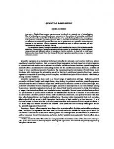
Thanks to the methods described in this paper, the application of D-vine quantile regression is no longer restricted to continuous data sets. We investigate the bike sharing data set from the UCI machine learning repository (Lichman, 2013), first analyzed in Fanaee-T and Gama (2013). It contains information on rental counts from the bicycle sharing system Capital Bikeshare offered in Washington, D.C., together with weather and seasonal information. As a response for the quantile regression we choose the daily count of bike rentals, observed in the years 2011-2012 (731 observations). They are displayed in the left panel of Figure 1.

detrended rental count

rental count

7500

5000

2500

1.5

1.0

0.5

0.0

0 Jan 11

Jul 11

Jan 12

Jul 12

Jan 13

date

Jan 11

Jul 11

Jan 12

Jul 12

Jan 13

date

Figure 1: Observed (left) and detrended (right) bike rental counts in the years 2011-2012.

There is an obvious seasonal pattern and a linear trend reflecting a growth of the bike share system (visualized by the dashed line which is the least square linear line). While the seasonal pattern will be handled by the covariates, we cannot account for the linear trend. Therefore we remove the linear trend by dividing each observation by the least squares estimate of the linear trend. We use the division rather than the subtraction of the trend since the trend is a measure for the overall members of the bike sharing community and we are interested in the proportion of members renting bikes. The resulting detrended response is plotted in the right panel of Figure 1. For each day we have continuous covariates temperature (apparent temperature in Celsius), wind speed (in mph) and humidity (relative in %). Additionally, there is the discrete variable weather situation giving information about the overall weather with values 1 (clear to partly cloudy), 2 (misty and cloudy) and 3 (rain, snow, thunderstorm). Further, we have information 11

about the season (spring, summer, fall and winter), month and weekday of the observed day and an indicator whether the day is a working day. We applied all quantile regression methods discussed in this paper to the bike sharing data set for the quantile levels 0.1, 0.5 and 0.9 and use 10-fold cross-validation to evaluate their out-ofsample performance. Table 5 displays the corresponding averaged cross-validated tick-losses piq 1 ř731 piq ´ q (see e.g. Komunjer, 2013), given by 731 ˆα q, where ρα pyq “ ypα ´ 1py ă 0qq i“1 ρα py piq

denotes the check function, y piq is the i-th observation of the response and qˆα is the αquantile prediction. As before, the smallest losses and those which are not significantly larger than the smallest losses are printed in bold. Again, a Student’s t test at 5% level was used to test whether larger values are significantly larger than the smallest value in a row. α 0.1 0.5 0.9

PDVQR 0.039 0.082 0.042

NPDVQR 0.035 0.069 0.032

LQR 0.041 0.078 0.036

BAQR 0.035 0.064 0.032

NPQR 0.090 0.250 0.295

Table 5: Averaged in-sample tick-losses of the different quantile regression methods applied to the bike sharing data. NPDVQR and BAQR produce the best results, significantly beating LQR and NPQR. Between the two new D-vine copula based quantile regression methods introduced in this paper, the nonparametric one significantly outperforms the parametric one for α “ 0.5 and α “ 0.9. The reason is that most of the covariates enter the models in a non-monotone fashion, as we will see. The ranking of the covariates by the nonparametric sequential selection algorithm is: temperature — humidity — wind speed — month — weather situation — weekday — working day — season. In Figure 2 the influence of each of the covariates in the nonparametric D-vine quantile

0.5

0.9 0.5 0.1 0.5

0.0 20

30

40

80

0.1

100

1.0

0.5

0.9 0.5 0.1

20

30

Wed

0.1

Fri

0.9 0.5 0.1

Jul

Sep

quantile 1.0

quantile

0.9

0.9

0.5

0.5

0.1

0.1

0.0 yes

working day

spring

summer

fall

season

Figure 2: Influence of the different covariates on the response bike rentals using NPDVQR.

12

Nov

0.5

no

weekday

May

1.5

quantile 1.0

Sun

Mar

month

0.0 Mon

0.5

0.1

Jan

0.5

0.0 bad

0.9

0.5

0.0 10

1.5

quantile 1.0

quantile

0.9

wind speed

0.5

0.0

quantile 1.0

0.5

0

predicted count

predicted count

predicted count

60

1.5

weather situation

0.5

humidity

1.5

medium

0.9

0.0

40

temperature

good

quantile 1.0

0.5

0.0 10

predicted count

quantile 1.0

1.5

predicted count

1.0

1.5

predicted count

1.5

predicted count

predicted count

1.5

winter

regression model is visualized. To be precise, for a covariate Xj we calculate for all quantile piq piq levels α of interest qˆα “ FˆY´1 |X pα|X “ x q, i “ 1, . . . , 731, plot it against xij and add a smooth curve through the point cloud (fitted by loess). Figure 2 shows this for the quantile levels 0.1 (lower line), 0.5 (middle line) and 0.9 (upper line). Higher temperatures generally go along with more bike rentals, until it gets too warm. For temperatures higher than 32 degrees Celsius, each additional degree causes a decline in bike rentals. Similar observations can be made for humidity. Bike rentals increase up to a relative humidity of around 60% and decrease afterwards. Wind speed also has a strong influence with fewer bike rentals on windy days. It is not surprising that the warm summer months encourage many citizens to rent bikes while in the cold winter rentals decrease on average by approximately 60%. The inclination to borrow bikes seems to grow during the week. On the weekend however, especially the 10% quantile drops considerably, which may be explained by many people leaving the city to visit their families or doing leisure activities on weekends. This is also supported by the influence of variable working day, with a few more rentals on working days. The variables weather situation and season support the thesis that more people tend to rent bicycles when the weather is good. To investigate the differences between predictions of the various methods, we shall look more closely at the temperature variable. Figure 3 shows the effect of temperature on the predicted bike rentals using NPDVQR, PDVQR, LQR, BAQR and NPQR (from left to right). PDVQR

0.0

0.1 0.5

0.0

10

20

30

temperature

40

predicted count

predicted count

0.5

0.5

20

30

40

temperature

1.5

quantile

1.0 0.9 0.5 0.1 0.5

0.0

10

2.0

1.5

quantile

1.0 0.9

NPQR

2.0

1.5

quantile

1.0

BAQR

2.0

1.5

predicted count

1.5

predicted count

LQR

2.0

predicted count

NPDVQR 2.0

quantile

1.0 0.9 0.5 0.1 0.5

0.0

10

20

30

temperature

40

quantile

1.0 0.9

0.9

0.5

0.5

0.1

0.1

0.5

0.0

10

20

30

temperature

40

10

20

30

40

temperature

Figure 3: Influence of temperature on bike rentals for different quantile regression methods.

We see that the parametric D-vine as well as linear quantile regression are not really able to model the decline in rentals for very hot temperatures. Apart from assessing the influence of covariates on the response, quantile regression can also be used to predict quantiles of the response in different scenarios. Suppose we know tomorrow is going to be a warm August Saturday with medium humidity and low wind-speed. Then, using our nonparametric D-vine copula based quantile regression model, we would predict a median of 8872 bikes to be rented with 10%- and 90% quantiles 7431 and 10485, respectively. In contrast, for a cold December Monday with heavy snow and high wind-speed the three predicted quantiles would be 22, 674 and 1152. As an operator of such a bike sharing system we could thus adapt our supply of rental bikes to the predicted demand.

6

Conclusion and outlook

Two new methods to predict conditional quantiles in a mixed discrete-continuous setting are proposed. They are based on a D-vine copula model that is estimated either parametrically or nonparametrically. The simulation study shows that the non-parametric D-vine quantile regression provides fast and accurate predictions for non-linear relationships between the quantile and the covariates. The parametric approach is often less accurate. This is due to the fact that non-linear relationships imply non-monotonic effects of some covariates on the response, which cannot be adequately modeled by most of the popular parametric pair-

13

copula families. This shortfall could be overcome by using parametric families that allow for non-monotonic dependence patterns. Developing such models will be a promising path for future research.

Acknowledgment The third and fourth authors are supported by the German Research Foundation (DFG grants CZ 86/5-1 and CZ 86/4-1). Numerical calculations were performed on a Linux cluster supported by DFG grant INST 95/919-1 FUGG.

References Aas, K., Czado, C., Frigessi, A., and Bakken, H. (2009). Pair-copula constructions of multiple dependence. Insurance: Mathematics and Economics, 44(2):182–198. Bedford, T. and Cooke, R. M. (2002). Vines: A new graphical model for dependent random variables. Annals of Statistics, 30(4):1031–1068. Bernard, C. and Czado, C. (2015). Conditional quantiles and tail dependence. Journal of Multivariate Analysis, 138(C):104–126. Dette, H., Hecke, R. V., and Volgushev, S. (2014). Some comments on copula-based regression. Journal of the American Statistical Association, 109(507):1319–1324. Fanaee-T, H. and Gama, J. (2013). Event labeling combining ensemble detectors and background knowledge. Progress in Artificial Intelligence, pages 1–15. Fenske, N., Kneib, T., and Hothorn, T. (2012). Identifying risk factors for severe childhood malnutrition by boosting additive quantile regression. Journal of the American Statistical Association, 106(494):494–510. Geenens, G., Charpentier, A., and Paindaveine, D. (2017). Probit transformation for nonparametric kernel estimation of the copula density. Bernoulli, 23(3):1848–1873. Genest, C. and Neˇslehov´ a, J. (2007). A primer on copulas for count data. ASTIN Bulletin, 37(2):475–515. Hayfield, T. and Racine, J. S. (2008). Nonparametric econometrics: The np package. Journal of Statistical Software, 27(5). Hobæk Haff, I., Aas, K., and Frigessi, A. (2010). On the simplified pair-copula construction — simply useful or too simplistic? Journal of Multivariate Analysis, 101(5):1296–1310. Hofert, M., Kojadinovic, I., Maechler, M., and Yan, J. (2016). copula: Multivariate dependence with copulas. R package version 0.999-15. Hothorn, T., Buehlmann, P., Kneib, T., Schmid, M., and Hofner, B. (2016). mboost: Modelbased boosting. R package version 2.7-0. Joe, H. (1997). Multivariate models and multivariate dependence concepts. CRC Press. Killiches, M., Kraus, D., and Czado, C. (2017). Examination and visualisation of the simplifying assumption for vine copulas in three dimensions. Australian & New Zealand Journal of Statistics, 59(1):95–117.

14

Koenker, R. (2005). Quantile regression. Cambridge University Press, Cambridge, Cambridgeshire, United Kingdom. Koenker, R. (2011). Additive models for quantite regression: Model selection and confidence bandaids. Brazilian Journal of Probability and Statistics, 25(3):239–262. Koenker, R. (2015). quantreg: Quantile regression. R package version 5.19. Koenker, R. and Bassett, G. (1978). Regression quantiles. Econometrica, 46(1):33–50. Komunjer, I. (2013). Quantile prediction. In Handbook of Economic Forecasting, pages 767– 785. Elsevier. Kraus, D. and Czado, C. (2017). D-vine copula based quantile regression. Computational Statistics and Data Analysis, 110C:1–18. Li, Q., Lin, J., and Racine, J. S. (2013). Optimal bandwidth selection for nonparametric conditional distribution and quantile functions. Journal of Business & Economic Statistics, 31(1):57–65. Lichman, M. (2013). UCI machine learning repository. Nagler, T. (2017). A generic approach to nonparametric function estimation with mixed data. arXiv preprint, arXiv:1704.07457. Nagler, T. and Czado, C. (2016). Evading the curse of dimensionality in nonparametric density estimation with simplified vine copulas. Journal of Multivariate Analysis, 151:69– 89. Nagler, T., Schellhase, C., and Czado, C. (2017). Nonparametric estimation of simplified vine copula models: comparison of methods. arXiv preprint, arXiv:1701.00845. Nelsen, R. B. (2007). An introduction to copulas. Springer Science & Business Media. Onken, A. and Panzeri, S. (2016). Mixed vine copulas as joint models of spike counts and local field potentials. 30th Conference on Neural Information Processing Systems (NIPS 2016), Barcelona, Spain. URL: https://papers.nips.cc/paper/ 6069-mixed-vine-copulas-as-joint-models-of-spike-counts-and-local-field-potentials. pdf. Panagiotelis, A., Czado, C., and Joe, H. (2012). Pair copula constructions for multivariate discrete data. Journal of the American Statistical Association, 107(499):1063–1072. Schallhorn, N. (2017). D-vine quantile regression for mixed discrete and continuous data with applications to bank stress testing. Master’s thesis, Technische Universit¨at M¨ unchen, Germany. Sklar, A. (1959). Fonctions d´e repartition ´a n dimensions et leurs marges. Publications de l’Instutut de Statistique de l’Universit´e de Paris, 8:229–231. St¨ober, J. (2013). Regular vine copulas with the simplifying assumption, time-variation, and mixed discrete and continuous margins. Dissertation, Technische Universit¨at M¨ unchen, M¨ unchen. St¨ober, J., Joe, H., and Czado, C. (2013). Simplified pair copula constructions—limitations and extensions. Journal of Multivariate Analysis, 119:101–118.

15