D2.6 Prototype Software for Eigenvalue Problem Solvers - NLAFET

H2020–FETHPC–2014: GA 671633

D2.6 Prototype Software for Eigenvalue Problem Solvers

April 2018

NLAFET

D2.6: Prototypes for Eigenvalue Problem Solvers

Document information Scheduled delivery Actual delivery Version Responsible partner

2018-04-31 2018-04-27 1.1 UMU

Dissemination level PU — Public Revision history Date 2018-03-06 2018-04-14 2018-04-27 2018-04-27

Editor Bo Kågström Mirko Myllykoski Mirko Myllykoski Mirko Myllykoski

Status Draft Draft Final Correction

Ver. 0.1 0.2 1.0 1.1

Changes Initial structure. Final version for internal review. Final version. Corrections to Section 1.2.

Author(s) Mirko Myllykoski (UMU) Lars Karlsson (UMU) Bo Kågström (UMU) Mahmoud Eljammaly (UMU) Srikara Pranesh (UNIMAN) Mawussi Zounon (UNIMAN) Internal reviewers Sebastien Cayrols (STFC) Florent Lopez (STFC) Copyright c by the NLAFET Consortium, 2015–2018. This work is Its duplication is allowed only for personal, educational, or research uses. Acknowledgements This project has received funding from the European Union’s Horizon 2020 research and innovation programme under the grant agreement number 671633.

http://www.nlafet.eu/

1/31

NLAFET

D2.6: Prototypes for Eigenvalue Problem Solvers

Table of Contents 1 Introduction 1.1 The standard eigenvalue problem . . . . . . . . . . . . . . . . . . . . . . . 1.2 The generalized eigenvalue problem . . . . . . . . . . . . . . . . . . . . . . 1.3 StarPU runtime system . . . . . . . . . . . . . . . . . . . . . . . . . . . . . 2 Reduction to condensed forms 2.1 Standard algorithm . . . . . . . . . . . . . . . . . . . 2.2 Task-based Hessenberg reduction . . . . . . . . . . . 2.3 NUMA-aware Hessenberg reduction with auto-tuning 2.4 Distributed Hessenberg-triangular reduction . . . . . 2.5 Reflection-based Hessenberg-triangular reduction . . 3 Reduction to Schur forms 3.1 Task-based multishift QR algorithm . . . . . . 3.1.1 Task types . . . . . . . . . . . . . . . . 3.1.2 Subproblem states . . . . . . . . . . . 3.1.3 Events and state transitions . . . . . . 3.2 Distributed multishift QR and QZ algorithms

. . . . .

. . . . .

. . . . .

. . . . .

. . . . .

. . . . .

. . . . .

. . . . .

. . . . .

. . . . .

. . . . .

. . . . .

. . . . .

. . . . .

. . . . .

. . . . .

. . . . .

. . . . .

. . . . .

. . . . .

. . . . .

. . . . .

. . . . .

. . . . .

4 4 5 6

. . . . .

8 . 8 . 9 . 10 . 10 . 10

. . . . .

11 12 14 15 16 18

. . . . .

4 Symmetric eigenvalue problems 18 4.1 Novel algorithm with two-stage tridiagonal reduction . . . . . . . . . . . . 18 4.2 OpenMP task-based realization . . . . . . . . . . . . . . . . . . . . . . . . 19 5 Experimental results 5.1 Task-based Hessenberg reduction . . . . . . . . . . . . . . . . . . . . . . . 5.2 Task-based multishift QR algorithm . . . . . . . . . . . . . . . . . . . . . . 5.3 Symmetric eigenvalue problem solver . . . . . . . . . . . . . . . . . . . . .

19 19 22 26

6 Conclusion and future work

28

List of Figures 1 2 3 4 5 6 7 8 9 10 11

LAPACK layout versus tile layout. . . . . . . . . . . . . . . . . . . . . . An illustration of two iterations of the Hessenberg reduction algorithm. An illustration of a single iteration of the multishift QR algorithm. . . . The subproblem states and all possible state transitions. . . . . . . . . . Possible state transitions from the Bulges state. . . . . . . . . . . . . . . Strong scalability of the StarPU-based Hessenberg reduction algorithm. A runtime comparison between the StarPU-based Hessenberg reduction algorithm, LAPACK (with multi-threaded BLAS) and ScaLAPACK. . . A runtime comparison between the StarPU-based Hessenberg reduction algorithm and MAGMA. . . . . . . . . . . . . . . . . . . . . . . . . . . . Strong scalability of the StarPU-based multishift QR algorithm. . . . . A runtime comparison between the StarPU-based multishift QR algorithm, LAPACK (with multi-threaded BLAS) and ScaLAPACK. . . . . . . . . An example of a trace plot generated by the StarPU. . . . . . . . . . . .

http://www.nlafet.eu/

. . . . . .

7 8 12 15 17 20

. 21 . 22 . 23 . 24 . 25

2/31

NLAFET

12 13 14 15

D2.6: Prototypes for Eigenvalue Problem Solvers

An example of a trace plot generated by the StarPU when running in distributed memory mode. . . . . . . . . . . . . . . . . . . . . . . . . . . Performance of 2-stage DSYEVD when only eigenvalues are required. . . . Performance of 2-stage DSYEVD when both eigenvalues and eigenvectors are required. . . . . . . . . . . . . . . . . . . . . . . . . . . . . . . . . . . . . Performance details of the 2-stage DSYEVD when both eigenvalues and eigenvectors are required. . . . . . . . . . . . . . . . . . . . . . . . . . . . . .

. 26 . 27 . 27 . 28

List of Tables 1

Overall status of the task-based software components for non-symmetric eigenvalue problems. . . . . . . . . . . . . . . . . . . . . . . . . . . . . . . 29

http://www.nlafet.eu/

3/31

NLAFET

1

D2.6: Prototypes for Eigenvalue Problem Solvers

Introduction

The Description of Action (DoA) document states for deliverable D2.6: “D2.6: Prototype Software for Eigenvalue Problem Solvers Prototypes for reduction to non-symmetric condensed forms (Hessenberg and Hessenberg-triangular), for the symmetric eigenvalue problem and the nonsymmetric eigenvalue problems.” This deliverable is in the context of Task 2.3 (Eigenvalue Problem Solvers) and is based on the M18 deliverable D2.51 and further developments by the UMU and UNIMAN teams. The long-term goal is to develop and implement a full suite of task-based algorithms (at least where task-based algorithms prove to be superior) for the standard and generalized eigenvalue problems. The provided functionality should make it possible to compute all or a subset of the eigenvalues and associated subspaces or eigenvectors. The focus of the UMU team is on medium- to large-scale dense non-symmetric eigenvalue problems, while the UNIMAN team is working on symmetric counterparts. In this deliverable, we report progress on the symmetric and non-symmetric eigenvalue problems, including the reduction to Hessenberg and Hessenberg-triangular forms (a.k.a reduction to condensed forms) and the further reduction to Schur forms that reveal the eigenvalues along the block diagonal of the computed upper quasi-triangular matrices. These methods are based on two-sided matrix transformations (i.e., multiplicative updates applied from both the left and the right), which often lead to task graphs with complex data dependencies and limited degrees of concurrency. Such computations can therefore be challenging to run efficiently on today’s and future extreme-scale HPC systems.

1.1

The standard eigenvalue problem

Given a square matrix A of size n × n, the standard eigenvalue problem (SEP) consists of finding eigenvalues λi ∈ C and associated eigenvectors 0 6= vi ∈ Cn such that Avi = λi vi . The eigenvalues are the n (potentially complex) roots of the polynomial det(A − λI) = 0 of degree n. There is often a full set of n linearly independent eigenvectors, but if there are multiple eigenvalues (i.e., if λi = λj for some i 6= j) then there might not be a full set of independent eigenvectors. Reduction to Hessenberg form. The dense matrix A is condensed to Hessenberg form by computing a Hessenberg decomposition A = Q1 HQH 1 , where Q1 is unitary and H is upper Hessenberg. This is done in order to greatly accelerate the subsequent computation of a Schur decomposition since when working on H of size n × n, the amount of work in each iteration of the QR algorithm (see Section 3) is reduced from O(n3 ) to O(n2 ) flops. 1

Deliverable D2.5: Report on computation of eigenvectors and reordering of eigenvalues in Schur and generalized Schur forms. Includes evaluation of the scalability and tunability of the prototype software developed.

http://www.nlafet.eu/

4/31

NLAFET

D2.6: Prototypes for Eigenvalue Problem Solvers

Reduction to Schur form. Starting from the Hessenberg matrix H we compute a Schur decomposition H = Q2 SQH 2 , where Q2 is unitary and S is upper triangular. The eigenvalues of A can now be determined as they appear on the diagonal of S, i.e., λi = sii . For real matrices there is a similar decomposition known as the real Schur decomposition H = Q2 SQT2 , where Q2 is orthogonal and S is upper quasi-triangular with 1 × 1 and 2 × 2 blocks on the diagonal. The 1 × 1 blocks correspond to the real eigenvalues and each 2 × 2 block corresponds to a pair of complex conjugate eigenvalues. Eigenvalue reordering and invariant subspaces. Given a subset consisting of m of the eigenvalues, we can reorder the eigenvalues on the diagonal of the Schur form by constructing a unitary matrix Q3 such that Sˆ11 Sˆ12 H Q 0 Sˆ22 3

"

S = Q3

#

and the eigenvalues of the m × m block Sˆ11 are the selected eigenvalues. The first m columns of Q3 span the invariant subspace associated with the selected eigenvalues. Computation of eigenvectors. Given a subset consisting of m of the eigenvalues λi for i = 1, 2, . . . , m and a Schur decomposition A = QSQH , we can compute for each λi an eigenvector vi 6= 0 such that Avi = λi vi by first computing an eigenvector wi of S and then transform it back to the original basis by multiplication with Q.

1.2

The generalized eigenvalue problem

Given a square matrix pencil A−λB, where A, B ∈ Cn×n , the generalized eigenvalue problem (GEP) consists of finding generalized eigenvalues λi ∈ C and associated generalized eigenvectors 0 6= vi ∈ Cn such that Avi = λi Bvi . The eigenvalues are the n (potentially complex) roots of the polynomial det(A − λB) = 0 of degree n. There is often a full set of n linearly independent generalized eigenvectors, but if there are multiple eigenvalues (i.e., if λi = λj for some i 6= j) then there might not be a full set of independent eigenvectors. At least in principle, a GEP can be transformed into a SEP provided that B is invertible, since Av = λBv ⇔ (B −1 A)v = λv. However, in finite precision arithmetic this practice is not recommended.

http://www.nlafet.eu/

5/31

NLAFET

D2.6: Prototypes for Eigenvalue Problem Solvers

Reduction to Hessenberg-triangular form. The dense matrix pair (A, B) is condensed to Hessenberg-triangular form by computing a Hessenberg-triangular decomposition A = Q1 HZ1H , B = Q1 Y Z1H , where Q1 , Z1 are unitary, H is upper Hessenberg, and Y is upper triangular. This is done in order to greatly accelerate the subsequent computation of a generalized Schur decomposition. Reduction to generalized Schur form. Starting from the Hessenberg-triangular pencil H − λY we compute a generalized Schur decomposition H = Q2 SZ2H ,

Y = Q2 T Z2H ,

where Q2 , Z2 are unitary and S, T are upper triangular. The eigenvalues of A − λB can now be determined from the diagonal element pairs (sii , tii ), i.e., λi = sii /tii (if tii 6= 0). If sii 6= 0 and tii = 0, then λi = ∞ is an infinite eigenvalue of the matrix pair (S, T ). (If both sii = 0 and tii = 0 for some i, then the pencil is singular and the eigenvalues are undetermined; all complex numbers are eigenvalues). For real matrix pairs there is a similar decomposition known as the real generalized Schur decomposition H = Q2 SQT2 ,

Y = Q2 T Z2T ,

where Q2 , Z2 are orthogonal, S is upper quasi-triangular with 1 × 1 and 2 × 2 blocks on the diagonal, and T is upper triangular. The 1 × 1 blocks on the diagonal of S − λT correspond to the real generalized eigenvalues and each 2 × 2 block corresponds to a pair of complex conjugate generalized eigenvalues. Eigenvalue reordering and deflating subspaces. Given a subset consisting of m of the generalized eigenvalues, we can reorder the generalized eigenvalues on the diagonal of the generalized Schur form by constructing unitary matrices Q3 and Z3 such that "

S − λT = Q3

Sˆ11 − λTˆ11 Sˆ12 − λTˆ12 H Z 0 Sˆ22 − λTˆ22 3 #

and the eigenvalues of the m × m block pencil Sˆ11 − λTˆ11 are the selected generalized eigenvalues. The first m columns of Z3 spans the right deflating subspace associated with the selected generalized eigenvalues. Computation of generalized eigenvectors. Given a subset consisting of m of the eigenvalues λi for i = 1, 2, . . . , m and a generalized Schur decomposition A − λB = Q(S − λT )Z H , we can compute for each λi a generalized eigenvector vi 6= 0 such that Avi = λi Bvi by first computing a generalized eigenvector wi of S −λi T and then transform it back to the original basis by multiplication with Z.

1.3

StarPU runtime system

Two of the main software components presented in this deliverable report (task-based Hessenberg reduction and task-based multishift QR algorithm) are built on top of the StarPU runtime system [3]. The main difference between the previous algorithms and our http://www.nlafet.eu/

6/31

NLAFET

D2.6: Prototypes for Eigenvalue Problem Solvers

(a) LAPACK layout

(b) Tile general layout

(c) Tile triangular layout

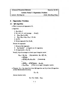
Figure 1: LAPACK layout versus tile layout. task-based approach is that we have expressed our algorithms in the terms of the sequential task-flow model (STF model). The STF model encapsulated the various computational operations inside tasks that are created/inserted in a sequentially consistent order. A runtime system can thus automatically deduce all task dependencies by analyzing the data flow. While LAPACK stores the matrix in a column-major order, we store the matrix in tiles, which are small square blocks of the matrix stored in a contiguous memory region as illustrated in Figure 1. These tiles can be loaded into the cache memory efficiently and operated on with little risk of eviction. Hence, the use of the tile layout reduces the number of cache misses and translation lookaside buffer (TLB) misses, reduces false sharing, and increases the potential for prefetching. StarPU uses data handles to model the data flow between tasks and each tile is registered with StarPU using a data handle. This means that StarPU considers each tile to be an independent unit of data. StarPU encapsulates various computational kernels inside codelets. Each codelet can have multiple implementations and StarPU is capable of determining which implementation (and which computational resource) should be used in a given situation. This requires that an algorithm specifies some extra information in terms of performance models that provide an estimate for the task execution time. Certain task schedulers (e.g., pheft and dmdasd) can make more informed scheduling decisions when this information is provided. When an algorithm inserts a task, it specifies the associated codelet and a list of data handles. The same list of data handles acts as an argument list for the codelet when the task is later issued to a worker. StarPU uses this same argument list when it deduces the task dependencies. For example, if two tasks are given a same data handle in their argument lists (i.e., they operate on the same tile), then depending on the order in which the tasks are inserted and various data access mode flags, an implicit data dependency may be induced between the two tasks. StarPU-MPI is an extension that integrates StarPU with the MPI message passing system. An algorithm may define all MPI rank to MPI rank communications explicitly or the algorithm may simply define how the data is distributed among the MPI ranks and let StarPU handle all necessary communication. In the latter case, the algorithm must provide an unique tag and a rank (i.e. owner) for each data handle. As explained in our earlier technical report (see [19]), our current implementation uses the second approach. We define the data distribution by splicing adjacent tiles into sections such that tiles that belong to the same section have a common owner (rank). More specifically, a matrix of size n × n is divided into sections of size s × s which are then further divided into tiles of size t × t. Each section resides on some MPI rank. We tried to reduce the overhead by

http://www.nlafet.eu/

7/31

NLAFET

D2.6: Prototypes for Eigenvalue Problem Solvers

parallel scheduling context

regular scheduling context

process panel update trail

right update

process panel update trail

right update

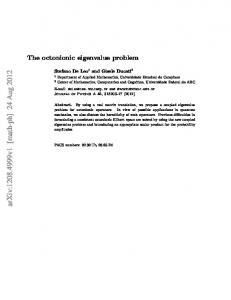
Figure 2: Top left: Sketch of how the matrix A is partitioned in one of the iterations. The panel is shown in red, the trailing matrix is shown in yellow, and the part that is only updated from the right is shown in green. Bottom left: Sketch of the partitioning in the subsequent iteration. Right: Illustration of how the three primary tasks (process the panel, update the trailing matrix, and apply the right updates) from two adjacent iterations are dependent and to which scheduling context each one is inserted. making each MPI rank register only those tiles that it actually needs. However, some tiles are needed by multiple MPI ranks. This is why we implemented a separate subsystem that will automatically register a “placeholder” data handle when an MPI rank that does not own a tile requests a data handle to it. When this happens, the subsystem also communicates the correct tag and rank to StarPU.

2

Reduction to condensed forms

Hessenberg algorithms are initially used for transforming A to Hessenberg form H and transforming (A, B) to Hessenberg-triangular form (H, Y ) before we apply the QR and QZ algorithms, respectively. They are also used for small to medium reductions in the aggressive early deflation (AED) processes for SEP and GEP. In particular, a task-based Hessenberg algorithm will be a necessary component in the task-based multishift QR algorithm which is discussed in Section 3.

2.1

Standard algorithm

Recall that the standard algorithm for reducing a matrix to upper Hessenberg form [20] proceeds in iterations, each one reducing b consecutive columns of A ∈ Rn×n as illustrated in Figure 2. Each iteration is divided into three separate steps: 1. Process the panel. Reduce the current panel (red in Figure 2) by constructing and applying b Householder reflectors. Aggregate the reflectors into a compact WY representation I − V T V T , where T ∈ Rb×b and V ∈ Rn×b has a very special pattern of zero entries. Compute and return the product Y = AV T and update only the panel. The performance of the panel processing is severely limited by the need to perform a large matrix-vector multiplication per column involving the unreduced http://www.nlafet.eu/

8/31

NLAFET

D2.6: Prototypes for Eigenvalue Problem Solvers

part of the matrix (a.k.a trailing matrix). In total, approximately 20% of the flops (regardless of the size of the matrix) are attributable to these n − 2 memory-bound level-2 BLAS operations. 2. Update the trailing matrix. Update the trailing matrix (yellow in Figure 2) from both sides by the (conceptual) update formula A ← (I − V T V T )T (A − Y V T ). Since the panel itself was updated already during the panel processing, the panel is excluded from this update. 3. Update the top part from the right. The top part (green in Figure 2) is subject only to updates from the right and the (conceptual) update formula is A ← A − Y V T. The right part of Figure 2 shows that the third step never feeds back into the first two and is therefore not as critical (in terms of scheduling) as the other two.

2.2

Task-based Hessenberg reduction

In principle at least, the matrix can be partitioned into tiles and transformed into a taskbased algorithm operating on the level of individual tiles. However, since approximately 20% of the flops are performed during panel processing as n − 2 matrix-vector multiplications, the performance hinges on the rate at which these (memory-bound) flops can be executed. There is little to be gained, except additional parallel overhead, in executing a matrix-vector multiplication as a set of dynamically scheduled tasks as opposed to a simpler parallelization scheme that has less task scheduling overhead. In addition, although some level-2 and level-3 BLAS operations from different steps (and even different panels) can be overlapped, the large matrix-vector multiplications still end up forming significant bottlenecks for the performance of the implementation. Based on this insight, we have made use of the scheduling context and the parallel task scheduler features in StarPU. Scheduling contexts are used to control the distribution of computational resources. Each scheduling context manages a set of (CPU and/or GPU) workers and a task that is inserted to a given scheduling context gets scheduled to one of the workers managed by the context. Regular schedulers assume that all CPU codelet implementations are sequential, i.e., they do not express any inner-task (thread-level) parallelism. A parallel task scheduler, on the other hand, joins several CPU workers to so-called combined workers and each task is scheduled to one of the underlying CPU workers or one of the combined workers. The runtime system guarantees that a CPU core is not simultaneously allocated for multiple tasks. This means that a task, that is inserted to a scheduling context with a parallel task scheduler, can express inner-task parallelism (within the bounds specified by the runtime system) without causing CPU core oversubscription or other thread affinity problems. We view each panel processing step as one (massive) task for which we provide both an OpenMP-based parallel CPU implementation and a cuBLAS-based parallel GPU implementation for the StarPU system to choose from at runtime. The OpenMP implementation first copies the trailing matrix to physically local memory in order to maximize the memory bandwidth of the b matrix-vector multiplications in the panel processing step. http://www.nlafet.eu/

9/31

NLAFET

D2.6: Prototypes for Eigenvalue Problem Solvers

The GPU implementation performs the matrix-vector multiplications ”in-place“, i.e., the implementation does not copy the trailing matrix to physically local memory. For this, a custom CUDA kernel is required but the performance of this custom CUDA kernel is comparable to cuBLAS (cublasDgemv). Similarly, we provide an OpenMP-based parallel implementation of Step 2 along with a cuBLAS-based parallel GPU implementation. The critical tasks (i.e., the tasks from Steps 1 and 2) are inserted to a parallel scheduling context (using a parallel task scheduler; peager or pheft) which consists of a GPU (if one exists in the machine) along with a subset of the CPU cores distributed over the NUMA islands. Step 3 is further decomposed into a set of sequential tasks and inserted to a regular scheduling context (using a regular task scheduler; prio or dmdasd) which consists of the remaining GPUs and CPU cores. The GPU implementation of the tasks in Step 3 uses cuBLAS. The regular scheduling context inherits the workers from the parallel scheduling context once all panel processing and trailing matrix update steps have completed. All tasks have performance models implemented.

2.3

NUMA-aware Hessenberg reduction with auto-tuning

We implemented a NUMA-aware variant of the standard algorithm for small problems which targets shared memory systems. The idea is to use this fine-grained parallelism implementation in the AED to speed it up. Paper [12] presents the implementation details of the algorithm and evaluates its tunability. In addition, an off-line auto-tuning mechanism is proposed to tune the new implementation’s parameters. We concluded from paper [12] that it is difficult to apply standard auto-tuning methods to tune the parameters of the new implementation. So in paper [11] (a condensed version of NLAFET Working Note 18 [13]) we proposed an auto-tuning framework which helps tuning the parameters of the new implementation efficiently. The framework reveals the underling sub-problems and allows applying standard tuning methods on them. We will use the framework to investigate the best on-line auto-tuning method for the new implementation.

2.4

Distributed Hessenberg-triangular reduction

Given a real matrix pencil A − λB of size n × n, the software available in repository NLAFET/GEVP-PDHGEQZ on NLAFET’s GitHub page computes a Hessenberg-triangular decomposition A − λB = Q(S − λT )Z T , where Q, Z are orthogonal, S is upper Hessenberg, and T is upper triangular. The software targets distributed memory and the parallel programming is done in pure MPI. A novel wavefront scheduling strategy is introduced. The parallel algorithm is described and evaluated against the state of the art in [6].

2.5

Reflection-based Hessenberg-triangular reduction

The algorithm and software introduced in Section 2.4 has limited scalability due to data dependences that restrict the degree of concurrency, bound the arithmetic intensity, and require frequent inter-process communication. We have therefore, together with external collaborators, developed a novel algorithm for Hessenberg-triangular reduction that circumvents some major bottlenecks in the original algorithm. The technical report [9] http://www.nlafet.eu/

10/31

NLAFET

D2.6: Prototypes for Eigenvalue Problem Solvers

describes the new algorithm and evaluates it in a sequential setting against the state of the art. The main conclusion is that even though the algorithm requires approximately twice as much arithmetic as the state of the art, the sequential runtime is nevertheless competitive. We are currently developing a task-based parallel formulation.

3

Reduction to Schur forms

A modern small-bulge multishift QR/QZ algorithm consists of two main components: aggressive early deflation and pipelined bulge-chasing (also known as QR/QZ iterations). Small-bulge multishift and AED are techniques meant to speed up the convergence relative to the textbook implicit single- or double-shift QR/QZ algorithms. These techniques also make the algorithms more suitable for efficient implementations on shared memory as well as on distributed memory parallel computer systems since they improve the arithmetic intensity [7, 8, 14, 15]. The following introductory discussion focuses on the multishift real QR algorithm with AED for the standard eigenvalue problem, but all ingredients and arguments have their counterparts for the generalized eigenvalue problem and the multishift QZ algorithm with AED [4, 5, 16]. The real QR algorithm takes a Hessenberg matrix H as input and reduces it to real Schur form H = QSQT , where S is upper quasi-triangular. If a sub-diagonal element hj+1,j of H is zero, then H can be partitioned into a block upper triangular matrix as in "

#

H11 H12 H= , 0 H22 where H11 is j × j. The problem of reducing H thereby decouples into the two smaller independent problems of reducing H11 and H22 . A Hessenberg matrix is said to be unreduced if none of the sub-diagonal elements are zero. An active region is a contiguous square submatrix on the diagonal of H that is unreduced and of maximal size (which means that it cannot be increased and remain unreduced). If H itself is unreduced, then it has one active region that covers the entire matrix. When H is fully reduced, then (and only then) are there no active regions. Converged eigenvalues are normally detected during AED, in which case the active region will deflate (shrink) from the bottom. In some (rare) instances, a subdiagonal element might be flushed to zero during bulge-chasing, thereby triggering a decoupling of the problem. This is called a vigilant deflation. The goal of the QR algorithm is to perform AEDs and bulge-chasing in the various active regions until either all eigenvalues have been deflated or a failure to converge is detected. An AED is performed inside a window, i.e., a square contiguous submatrix on the diagonal, called the AED window. This window is small relative to the size of H and is located at the bottom right corner of an active region. The AED process can be outlined as follows. Initially, the window (dashed outline in the middle of Figure 3) is reduced to Schur form (e.g., by a recursive application of the multishift QR algorithm). When the corresponding out-of-window updates are applied2 , a spike forms immediately to the left of the window (middle of Figure 3). By systematic application of eigenvalue reordering within the window, each eigenvalue computed for the window is tested to determine if it is also an eigenvalue for H (and by extension for A). All converged eigenvalues, i.e., eigenvalues that are ready to deflate (highlighted in green in Figure 3) end up at the 2

In practice, the matrix is not updated at this point.

http://www.nlafet.eu/

11/31

NLAFET

D2.6: Prototypes for Eigenvalue Problem Solvers

Figure 3: An illustration of a single iteration of the multishift QR algorithm with AED. From left to right: original A in Hessenberg form H, AED window including the spike (converged eigenvalues highlighted in green, failed eigenvalue candidates highlighted in red), and pipelined QR iteration with two bulge-chasing windows. Note how the active region (dashed outline) shrinks after the AED process managed to deflate a set of eigenvalues. bottom of the window. The corresponding elements of the spike will be so small that they can safely be set to zero thus forming a fully reduced block in the lower right corner of the window. The top part of the window and what remains of the spike is returned to Hessenberg form by a Hessenberg reduction. Finally, the transformations applied during the AED are applied to the out-of-window parts of H from left and right and to Q from the right. There is one special case that bears to mention. If no eigenvalues are deflated, then there is no need to perform any modifications to H at all and therefore all the within-window computations mentioned above should be performed on a temporary copy of the window in order to preserve the original data. In most cases, an AED does not deflate an entire window. The undeflated eigenvalues computed for the window can be used as shifts in a QR iteration. The main point of a small-bulge multishift QR/QZ algorithm is to use multiple shifts per QR iteration, instead of only two shifts as in the implicit double-shift algorithm. The shifts are introduced in pairs in the upper left corner of an active region. Each shift pair forms a 3 × 3 bulge on the subdiagonal. These bulges are chased along the subdiagonal in tightly coupled chains as illustrated in the rightmost illustration of Figure 3. The resulting updates (to effect a similarity transformation) are initially restricted to a bulge-chasing window and the out-of-window updates are delayed and applied in accumulated form using matrix multiplication.

3.1

Task-based multishift QR algorithm

The small-bulge multishift QR algorithm shares similarities with eigenvalue reordering (part of deliverable D2.5, see also [18, 19]) but introduces some additional challenges. Except for the potential failure when swapping adjacent eigenvalues, the eigenvalue reordering problem can be completely expressed as a task graph before any tasks are actually executed. This is not doable for the QR algorithm due to inherently data-dependent branch points. For example, it is impossible to predict how many eigenvalues an AED will deflate. If only a few eigenvalues were deflated, then there are sufficiently many shifts to motivate performing a QR iteration. On the other hand, if many eigenvalues were deflated, then it is probably better to perform another round of AED rather than a QR http://www.nlafet.eu/

12/31

NLAFET

D2.6: Prototypes for Eigenvalue Problem Solvers

iteration. The task graph must therefore be generated in stages with partial synchronization between them in order to wait for the data that is necessary to determine the direction of a particular branch. In order to maximally exploit parallelism, our task-based implementation can make progress on all active regions at the same time. The main thread, which inserts all the tasks, cannot simply insert all the tasks for one active region before continuing with the next. Since the main thread must periodically wait for certain tasks to complete, such a strategy would not be able to overlap computations in several active regions to any significant degree. We therefore adopt an event-driven architecture. The main thread maintains a list of subproblems. Initially, there is one subproblem corresponding to the problem of reducing the entire matrix H to Schur form. Over time, this list might grow and shrink as new subproblems (active regions) appear (by vigilant deflation) and disappear (by converging). Each subproblem is associated with an active region and is at any given moment in one of a finite number of distinct states. In addition, each subproblem has a vigilant deflation vector associated with it. The purpose of this vector will be explained later. The main thread does not perform any computations or communications. It simply inserts tasks that are later scheduled to the workers and initializes detached communication requests 3 . More specifically, the purpose of the main thread is to detect events (e.g., that certain tasks have completed or that a vigilant deflation has been detected) and then execute a corresponding state transition function. A state transition function (potentially) changes the state of the subproblem and often triggers some additional actions (e.g., insertion of StarPU tasks or creation of new subproblems). Algorithm 1 outlines the control flow of the main thread. First a subproblem for the entire matrix is created and placed in an otherwise empty list of subproblems. The main loop continues until the list is exhausted (or a failure is detected). In each iteration, the list of subproblems is scanned and events for each subproblem are detected and handled. Normally, either no event is detected or there is an event that simply triggers a state transition. However, there are three states that in addition also affects the list of subproblems itself. The converged state triggers the removal of the subproblem. The failed state triggers an early termination of the entire algorithm. The children state triggers the insertion of newly created subproblems into the list. The newly created subproblems are immediately ready for state transitions and the possible state transitions do not block the main thread, therefore it makes sense to process them immediately (see line 16 of Algorithm 1). There are two variants of the event handler (the choice is up to the user): one that is blocking and another that is non-blocking. The latter is preferred when vigilant deflations are likely to occur. The blocking handler waits (blocks) on a subproblem until an event occurs. The non-blocking handler checks (without blocking) if an event has occurred and otherwise immediately returns (which will cause the main thread to move on to the next subproblem). In Section 3.1.1 we describe the various StarPU task types of our implementation. The various subproblem states are described in Section 3.1.2 and the events and state 3

A detached communication request is a special form of an asynchronous/non-blocking communication. It differs from a regular asynchronous MPI communication request in such a way that the actual MPI API calls are detached from the thread that initialized the communication. Instead, the actual communication (and the related wait/test phase) is initialized internally inside StarPU and the related resources are automatically released once the communication has completed.

http://www.nlafet.eu/

13/31

NLAFET

D2.6: Prototypes for Eigenvalue Problem Solvers

Algorithm 1: The control flow of the main thread. 1 Let L be an empty list of subproblems; 2 Create a subproblem S for the entire matrix H with the state set to bootstrap; 3 Insert S into L; 4 while L is not empty do 5 for each subproblem S in L do 6 s ← State(S); 7 Run the event handler for state s on subproblem S; 8 t ← State(S); 9 if t = converged then 10 Remove S from L; 11 else if t = failed then 12 Return failure; 13 else if t = children then 14 N ← Children(S); 15 Remove S from L and insert the (elements of the) list N in its place; 16 The next iteration begins from the first element of N ; 17

Return success;

transitions that can take place are described in Section 3.1.3. 3.1.1

Task types

There are five task types. Three types for operations on windows and two types for out-of-window updates of H as well as updates of Q. The window-related task types are described below. Small QR tasks run a sequential multishift QR algorithm on a window that spans the entire active region. If the QR algorithm converges, then the window will be fully reduced (otherwise a failure is recorded). These tasks are implemented by a call to the dlahqr LAPACK routine. AED tasks perform aggressive early deflation on a window located at the bottom right corner of the active region. An AED task potentially deflates eigenvalues (and thereby shrink the active region). Only in the event of deflation does an AED task give rise to out-of-window updates. At this stage of development, these tasks are implemented by a call to the dlaqr3 LAPACK routine. Bulge-chasing tasks introduce/chase/annihilate chains of bulges in a window. Subdiagonal elements that are flushed to zero are marked in the vigilant deflation vector. These tasks are implemented by calling (a slightly modified version of) the dlaqr6 routine from ScaLAPACK 2.0.2. The update-related task types are described below. Right-hand side update tasks update H or Q from the right following some window operation. These tasks are implemented by a call to the dgemm BLAS routine (for CPUs) or the cublasDgemm cuBLAS routine (for GPUs). http://www.nlafet.eu/

14/31

NLAFET

D2.6: Prototypes for Eigenvalue Problem Solvers

New

Small

Converged

AED

Bulges Failure

Bootstrap

Children

Figure 4: The subproblem states and all possible state transitions. Left-hand side update tasks update H from the left following some window operation. These tasks are implemented by a call to the dgemm BLAS routine (for CPUs) or the cublasDgemm cuBLAS routine (for GPUs). Both of the update task types have performance models. 3.1.2

Subproblem states

A subproblem is, at any given moment, in one of the following states (see Figure 4): The Bootstrap state indicates that the subdiagonal may contain zeros and must therefore be scanned in order to locate all active regions. This state is used only for the first subproblem. The New state indicates that the subproblem is ready for a new main iteration. That is, the subproblem is at a branch point where a decision about what to do next needs to be made based on the size of the active region. The Small state indicates that the active region is being reduced by a small QR task. The AED state indicates that the subproblem is at a branch point following an AED. A decision about what to do next must be made based on the number of eigenvalues deflated by the AED. The Bulges state indicates that bulges are being chased in the active region. This state may also be entered from the Bootstrap state even though there is technically no bulge-chasing taking place at that point. The Children state indicates that the subproblem has split into several smaller subproblems due to vigilant deflation(s). The Converged state indicates that the subproblem has been solved (all eigenvalues have converged). The Failed state indicates that a small QR task failed to converge. http://www.nlafet.eu/

15/31

NLAFET

3.1.3

D2.6: Prototypes for Eigenvalue Problem Solvers

Events and state transitions

The list below describes all possible state transitions (see Figure 4). Each transition is defined by the event that triggers it, the state it transitions to, and the action that is performed before the transition. • Bootstrap → Bulges Triggered immediately. The associated action is to scan the subdiagonal for zeros and mark all zeros in the vigilant deflation vector. • New → Small Triggered if the dimension of the active region is below a certain threshold. The associated action is to insert a small QR task covering the entire active region and all associated left and right updates of H and right updates of Q. • New → AED Triggered if the dimension of the active region is above a certain threshold. The associated action is to insert an AED task covering an AED window at the bottom right corner of the active region. • Small → Converged Triggered if the small QR task reported success. There is no associated action. • Small → Failed Triggered if the small QR task reported failure. There is no associated action. • AED → New Triggered if the number of eigenvalues deflated by the AED is above a certain threshold. The associated action is to insert the left and right update tasks for H and the right update tasks for Q. • AED → Bulges Triggered if the number of eigenvalues deflated by the AED is below a certain threshold. The first associated action (which is performed only if at least one eigenvalue converged) is to insert the related left and right update tasks for H and the right update tasks for Q. The second associated action is to insert bulge-chasing tasks and the associated left and right update tasks for H and the right update tasks for Q. • Bulges → New Triggered when all bulge-chasing tasks have completed and no vigilant deflations are detected. There is no associated action. • Bulges → Children Triggered when vigilant deflation(s) are detected. A list of subproblems is created, the last of which contains the remaining bulges (if any). All new subproblems are in the New state, except for the last subproblem which will be in the Bulges state if there are any unexecuted bulge-chasing tasks. In most cases, a task is simply given a special status tracking data handle and the task stores the outcome of the related computation to this data handle. The main thread

http://www.nlafet.eu/

16/31

NLAFET

D2.6: Prototypes for Eigenvalue Problem Solvers

No deflation

Deflated Fully acquired

Deflated Partially acquired

Bulges

Bulges

Bulges

New

Children

Children

New

New

New

New

New

Bulges

Figure 5: Possible state transitions from the Bulges state. From top down: Subproblem in the Bulges state (two concurrent bulge-chasing windows) and the vigilant deflation vector segments (segments that are involved with last bulge-chasing window are highlighted in red); subproblem and the vigilant deflation vector after the state transition (acquired segments highlighted in green, others segments in highlighted in red); and a matching state transition graph. From left to right: The vigilant deflation check vector was fully acquired and the subproblem did not decouple; the vigilant deflation check vector was fully acquired and the subproblem decoupled to three subproblems; and the vigilant deflation check vector was only partially acquired (one bulge-chasing window is still active) and the subproblem decoupled to three subproblems (one of which starts in the Bulges state). The scanning process and the point where the process was interrupted are visualized with dotted arrows.

http://www.nlafet.eu/

17/31

NLAFET

D2.6: Prototypes for Eigenvalue Problem Solvers

detects the related event by acquiring the data handle4 . The status tracking data handles and the vigilant deflation vector are communicated to the other MPI ranks using detached communication requests. The state transition from the Bulges state is slightly more complicated since the detected event(s) depends on the outcomes of multiple bulge-chasing tasks. Furthermore, the bulge-chasing stage is a relatively expensive computational operation and it may be sensible that the main thread detects only those events that have already occurred (i.e., the event detecting process is interrupted). Fortunately, all this can be accomplished relatively easily by acquiring the vigilant deflation vector. The main thread acquires (or tries to acquire) the deflation check vector in small segments. When configured to execute in the non-blocking mode, the main thread interrupts the scanning procedure if a segment is not ready (i.e., some bulge-chasing tasks that operate the matching section of the matrix have not yet completed and/or the related detached communication request has not yet completed). This process in visualized in Figure 5.

3.2

Distributed multishift QR and QZ algorithms

Distributed implementations of the QR [15] and QZ [5] algorithms based on MPI are available on NLAFET’s GitHub page as repositories NLAFET/SEVP-PDHSEQR-Alg953 re√ spectively NLAFET/GEVP-PDHGEQZ. Their designs are similar. Multiple (typically p where p is the number of processors) chains of bulges are chased in lock-step in multiple adjacent bulge-chasing windows in order to utilize all processes during the bulge-chasing phases. The AEDs are performed recursively in parallel after potentially redistributing the AED window to a subset of the process mesh to reduce the parallel overhead.

4

Symmetric eigenvalue problems

The symmetric eigenvalue problem is a special case of the standard eigenvalue problem — described in Section 1.1, where the matrix is symmetric. A symmetric eigenproblem involving dense matrices is commonly solved in three phases. During the first phase called “reduction”, the symmetric matrix is reduced to a tridiagonal matrix using an orthogonal transformation Q1 such that A = Q1 T QH 1 , where T is a tridiagonal matrix. Second, the eigenpairs (λ, E) of the tridiagonal matrix are computed; and finally the back transformation phase consists of computing the eigenvectors of the original matrix Z = Q1 E. The main contribution of this work is to improve the reduction to tridiagonal form and the back transformation phase.

4.1

Novel algorithm with two-stage tridiagonal reduction

Two-stage symmetric matrix reduction to tridiagonal form. State of the art algorithms for reduction of a symmetric matrix to tridiagonal form rely heavily on memorybound operations which have severe performance penalties. To address these limitations, we propose a two-stage approach where the matrix is first reduced to band form, then further from the band form to tridiagonal form. The first stage is compute-intensive and can be therefore performed efficiently using optimized level-3 BLAS kernels. It involves 4

The main thread must acquire a data handle before it can safely use its contents. By default, acquiring is a blocking operation (i.e., the main thread waits until the related task has completed). The main thread can also try to acquire a data handle in a non-blocking manner.

http://www.nlafet.eu/

18/31

NLAFET

D2.6: Prototypes for Eigenvalue Problem Solvers

construction of an orthogonal matrix Q1 , such that A = Q1 BQH 1 , and B is a symmetric banded matrix. The second stage which consists in obtaining the tridiagonal form B = Q2 T QH 2 , is still memory bound since we implement a column-wise bulge chasing approach. However we exploit cache friendly and data locality strategies to achieve an efficient implementation. Symmetric tridiagonal eigenvalue problem solver. In this work, we rely on the LAPACK divide and conquer kernel xSTEDC for the computation of the eigenvalues and eigenvectors of the tridiagonal matrix T . This decision is motivated by the efficiency of the divide and conquer algorithm available in LAPACK, and hence a new algorithm was not designed. Application of the orthogonal matrices Q1 and Q2 . When the eigenvector matrix Z are required, the eigenvector matrix E resulting from the eigensolver needs to be updated from the left by the Householder reflectors generated during the reduction phase as following: Z = Q1 Q2 E = (I − V1 T1 V1H )(I − V2 T2 V2H )E, where (V1 , T1 ) and (V2 , T2 ) represent the Householder reflectors generated during the first and second reduction stages, respectively.

4.2

OpenMP task-based realization

We have designed an OpenMP task-based version of a tile QR reduction algorithm (see Section 1.3 and Figure 1) in [10] for the first stage, and an OpenMP task-based and cache friendly variant of the bulge chasing algorithm initially introduced in [17] for the reduction to tridiagonal form — second stage. The associated software is available on the NLAFET’s GitHub page as repositories NLAFET/PLASMA/compute in real double precision (dsyevd), real single precision (syevd), complex double precision (zheevd), and complex single precision (cheevd).

5

Experimental results

Unless otherwise stated, all computational experiments were performed on a system called Kebnekaise, which is located in the High Performance Computing Center North (HPC2N) at Umeå University. Each regular compute node contains 28 Intel Xeon E5-2690v4 cores organized into 2 NUMA islands with 14 cores in each. The GPU nodes contain either two or four Kepler-based NVidia Tesla K80 GPUs with two GK210 GPU engines in each.

5.1

Task-based Hessenberg reduction

For these experiments, we compiled the test program using ICC 17.0.5.239 and linked it to StarPU 1.2.3, Intel MPI Version 2017 Update 4, MKL 2017.4.239 (either single-threaded or multi-threaded variant), CUDA toolkit 8.0.61 and MAGMA Bitbucket commit 7ba7d27 [1, 2]. Figure 6 shows the results of a conducted strong scalability experiment. For each measurement, an optimal number of CPU cores was allocated for the parallel scheduling context. This experiment did not involve any GPUs and at least one CPU core was http://www.nlafet.eu/

19/31

NLAFET

D2.6: Prototypes for Eigenvalue Problem Solvers

30000 20000 10000 5000

10

Speedup

8 6 4 2 0

5

10

15 # cores

20

25

Figure 6: Strong scalability of the StarPU-based Hessenberg reduction algorithm. always allocated for the regular scheduling context. When one takes into account the fact that the algorithm is inherently memory bound, the results show that the implementation scales reasonably well with larger matrices. However, the implementation clearly failed to scale equally well with smaller matrices. We also compared our StarPU algorithm against LAPACK (with multi-threaded BLAS; dgehrd and dormhr) and a state of the art MPI implementation that can be found from ScaLAPACK (pdgehrd and pdormhr). For each measurement, an optimal number of CPU cores was allocated for the parallel scheduling context. This experiment did not involve any GPUs and at least one CPU core was always allocated for the regular scheduling context. The results of the experiment are shown in Figure 7. The StarPU algorithm is more or less competitive with LAPACK and ScaLAPACK when the matrix is large. However, LAPACK and ScaLAPACK implementations scale better with small matrices (n = 5000 in particular) and thus outperform the StarPU implementation by a significant margin. The observed poor performance with the smaller matrices is due to the fact that the CPU panel reduction codelet implementation is optimized for larger matrices. When the matrix is large, it makes more sense to optimize the implementation to take a full advantage of the available NUMA islands. This is exactly what CPU panel reduction codelet implementation is designed to do. However, when the matrix is small, it makes more sense to take a full advantage of the available CPU caches. The CPU panel reduction codelet implementation is not designed to do this. The ScaLAPACK implementation, on the other hand, can take advantage of both the available NUMA islands and the CPU caches, as long as the block size is chosen optimally and the MPI processes are evenly distributed among the available NUMA islands. The same applies to the LAPACK implementation when it is combined with a high performance multi-threaded BLAS. The StarPU algorithm failed to outperform MAGMA (magma_dgehrd and magma_dorghr) http://www.nlafet.eu/

20/31

NLAFET

D2.6: Prototypes for Eigenvalue Problem Solvers

50 40 30 20 10 0

400

0

200 0

10 20 # cores

n = 20000

3000 2000 1000

0

10 20 # cores

n = 30000

12500 Runtime [s]

Runtime [s]

300 100

4000

0

n = 10000

500 Runtime [s]

Runtime [s]

n = 5000

StarPU LAPACK ScaLAPACK

10000 7500 5000 2500

0

10 20 # cores

0

0

10 20 # cores

Figure 7: A runtime comparison between the StarPU-based Hessenberg reduction algorithm, LAPACK (with multi-threaded BLAS) and ScaLAPACK.

http://www.nlafet.eu/

21/31

NLAFET

D2.6: Prototypes for Eigenvalue Problem Solvers

400

StarPU Magma

350

Runtime [s]

300 250 200 150 100 50 0

5000

10000 15000 Matrix dimension

20000

Figure 8: A runtime comparison between the StarPU-based Hessenberg reduction algorithm and MAGMA. on the Nvidia Tesla K80 GPUs. Nvidia’s CUDA profiler indicates that the problem is likely related to the number of CUDA and cuBLAS API calls the implementation makes (some of which came from the StarPU itself). We therefore performed the comparisons on a desktop machine with a Nvidia GeForce GTX1060 GPU that did not suffer from the API overhead to the same extent. The algorithm is inherently memory bound so the relatively low double precision floating-point performance of the Nvidia GeForce GTX1060 GPU (compared to the Nvidia Tesla K80 GPU) is unlikely to affect the outcome. The results are shown in Figure 8.

5.2

Task-based multishift QR algorithm

For StarPU and LAPACK experiments, we compiled the test program using ICC 17.0.5.239 and linked it to StarPU 1.2.3 and MKL 2017.4.239 (either single-threaded or multithreaded variant). For ScaLAPACK experiments, we compiled the test program using ICC 2017.1.132 and linked it to StarPU 1.2.3, OpenMP 2.0.1 and single-threaded MKL 2017.1.132. Figure 9 shows the results of a conducted strong scalability experiment. The implementation scales reasonably well with larger matrices but the scalability is not as good as hoped for with smaller matrices. As we will explain later, the poor scalability is mainly due to the fact that the AED is performed sequentially at this point in time. The StarPU algorithm was compared against LAPACK (with multi-threaded BLAS; dhseqr) and a state of the art MPI implementation that can be found from ScaLAPACK (pdhseqr). The results of the experiment are shown in Figure 10. Even though the StarPU implementation did not scale as well as hoped for with smaller matrix sizes, the implementation still managed to outperform LAPACK and ScaLAPACK implementations

http://www.nlafet.eu/

22/31

NLAFET

D2.6: Prototypes for Eigenvalue Problem Solvers

30000 20000 10000 5000

14 12 Speedup

10 8 6 4 2 0

5

10

15 # cores

20

25

Figure 9: Strong scalability of the StarPU-based multishift QR algorithm. by a significant margin. The reason why the LAPACK implementation outperforms the StarPU and ScaLAPACK implementations when using only one CPU core is probably that the QR algorithm is very sensitive to how various parameter values are chosen (the size of the AED window in particular). The LAPACK implementation has much more fine-tuned parameters and we have not invested a lot of time to tuning our StarPU implementation since some key components of the implementation are still incomplete. It should be noted that ScaLAPACK implementation performs the AED process in parallel. The fact that the sequential AED tasks form a performance bottleneck can be easily confirmed by observing the FxT trace plot shown in Figure 11. The experiment was performed on a desktop machine to keep the trace plot readable. A similar result can be obtained using the more high-end resources that are available at Kebnekaise. At first, the implementation manages to keep all worker occupied even when one worker is executing an AED task. However, the workers begin to come idle near the end of the experiment and this begins to happen even earlier stages when the number of workers larger than used here. The trace plot also shows that the algorithm performs several successive AED procedures. This indicates that the used AED window size is probably in a sweet spot between even smaller AED window sizes, that would lead to even more successive AED procedures, and larger AED window sizes, that would lead to less cache reuse. Furthermore, performing several smaller successive AED procedures can expose slightly more parallelism since the related off-diagonal updates are performed in parallel. Numerical experiments (and earlier research on the topic) indicate that the algorithm would converge with fewer QR iterations if the AED windows were larger (due to larger number of used shifts). However, the actual run time would be longer since the AED tasks are performed sequentially. Figure 12 shows a similar FxT trace plot in a situation where a 5000 × 5000 matrix is distributed over two MPI ranks. The matrix is distributed in 896 × 896 sections and each http://www.nlafet.eu/

23/31

NLAFET

D2.6: Prototypes for Eigenvalue Problem Solvers

n = 5000

n = 10000 200

30

Runtime [s]

Runtime [s]

40

20 10 0

0

150 100 50 0

10 20 # cores

0

n = 20000

n = 30000

500 250 0

StarPU LAPACK ScaLAPACK

3000 Runtime [s]

Runtime [s]

1000 750

0

10 20 # cores

10 20 # cores

2000 1000 0

0

10 20 # cores

Figure 10: A runtime comparison between the StarPU-based multishift QR algorithm, LAPACK (with multi-threaded BLAS) and ScaLAPACK.

http://www.nlafet.eu/

24/31

NLAFET

D2.6: Prototypes for Eigenvalue Problem Solvers

Figure 11: An example of a trace plot generated by the StarPU. The matrix dimension is 5000 × 5000. From top down: total number of inserted tasks that are not yet issued to the workers, number of tasks that are ready to be issued to the workers, total flop rate, memory manager (state, allocated memory and input/output memory bandwidth), statuses of the five CPU workers (active task and flop rate), and main thread status. The red color corresponds to idle time, light green colour to the AED tasks, teal (bluish green) colour to all update tasks and moss green (yellowish green) colour to the bulge-chasing tasks. The horizontal axis shows the wall-time in milliseconds.

http://www.nlafet.eu/

25/31

NLAFET

D2.6: Prototypes for Eigenvalue Problem Solvers

Figure 12: An example of a trace plot generated by the StarPU when running in distributed memory mode. section is divided into 224 × 224 tiles. Each MPI rank has a StarPU instance running with two CPU workers (one CPU core allocated for the main thread and the StarPUMPI communication thread per MPI rank). Again, the experiment was performed on a desktop machine to keep the trace plot readable. The reason why this figure is included is to demonstrate that the StarPU-MPI component of the software indeed functions as intended.

5.3

Symmetric eigenvalue problem solver

For these experiments, we compiled PLASMA using GCC 6.3 and linked to MKL 2018 for its single-thread BLAS functions and the multi-thread DSTEDC function required for the eigendecomposition of the resulting tridiagonal matrix. For a performance baseline, we used LAPACK 3.8.0 downloaded from Netlib, compiled using GCC 6.3, and linked to MKL 2018 for its multi-threaded BLAS functions. For the sake of comparison, we also report the performance of MKL’s DSYEVD routines. Figure 13 shows the performance of PLASMA’s DSYEVD routine when only the eigenvalues are required; and compares it against the performance of the LAPACK reference implementation linked with the vendor-provided BLAS and also against the performance of the vendor-provided LAPACK. On Broadwell, compared to the reference LAPACK implementation, PLASMA was able to more effectively utilize the 28 cores even with a relatively small matrix, while LAPACK takes up to 10x time to solve the same problem. We see that MKL has competitive performance compared to PLASMA’s DSYEVD. In fact Intel has optimized MKL and has implemented our 2-stage tridiagonal reduction algorithm to obtain such a high performance. Figure 14 shows the performance of PLASMA’s DSYEVD routine when both the eigenvalues and the eigenvectors are required. PLASMA’s DSYEVD shows in average 2x speedup over LAPACK’s DSYEVD. However compared to the results in Figure 13 the gap between LAPACK and PLASMA is considerably reduced. This can be explained by the fact that

http://www.nlafet.eu/

26/31

NLAFET

D2.6: Prototypes for Eigenvalue Problem Solvers

Figure 13: Performance of 2-stage DSYEVD when only eigenvalues are required.

Figure 14: Performance of 2-stage DSYEVD when both eigenvalues and eigenvectors are required.

http://www.nlafet.eu/

27/31

NLAFET

D2.6: Prototypes for Eigenvalue Problem Solvers

Figure 15: Performance details of the 2-stage DSYEVD when both eigenvalues and eigenvectors are required. the back transformation for the computation of the original matrix’s eigenvectors relies mainly on matrix-matrix operations and LAPACK is compiled with MKL multi-thread BLAS. MKL’s DSYEVD still shows a competitive performance but our implementation is slight more efficient. A detailed performance result for the PLASMA’s DSYEVD is depicted in Figure 15. One can observe that the percentage of time spent for the band reduction is almost constant while the percentage of time spent in the second stage, reduction to tridiagonal form is decreasing with the problem size. On the other hand the back transformation phase for the eigenvector computation is time consuming with increasing problem size. This exhibits a potential room for improvement, and in future work we will investigate novel approaches for a very efficient back transformation algorithm.

6

Conclusion and future work

We have developed a Hessenberg reduction implementation of the standard algorithm on top of StarPU. The implementation targets shared memory systems with or without GPUs. The StarPU algorithm is more or less competitive with LAPACK (with multithreaded BLAS) and ScaLAPACK when the matrix is large. The StarPU algorithm also outperforms MAGMA on some platforms. We are still working on improving the algorithm. In particular, the numerical results presented in Subsection 5.1 showed that the implementation does not scale well with small matrices. An obvious solution to this problem is to add a second CPU panel reduction codelet implementation that is optimized for smaller matrix sizes. StarPU could then use the provided performance models to choose the correct implementation for a given (trailing) matrix size. Also, the GPU side of the implementation is still slower that MAGMA on some platforms (Kepler-based Kebnekaise GPU nodes in particular). Nvidia’s CUDA profiler indicates http://www.nlafet.eu/

28/31

NLAFET

D2.6: Prototypes for Eigenvalue Problem Solvers

Memory model Component Shared Distributed Hessenberg reduction StarPU — Schur reduction StarPU StarPU-MPI Eigenvalue reordering StarPU StarPU-MPI Eigenvectors StarPU MPI + OpenMP

GPU Full Updates Updates —

Generalized EVP Ongoing Generalizable Supported Ongoing

Table 1: Overall status of the task-based software components for non-symmetric eigenvalue problems. The Full status indicates that all tasks have GPU/CUDA implementations. The Updates status indicates that the out-of-window update tasks have GPU/CUDA implementations. The Generalizable status indicates that the conversion from standard EVP to generalized EVP should be a straightforward process. that the problem is likely related to the number of CUDA and cuBLAS API calls the implementation makes. Some work has been invested to reducing the number of API calls and reducing their impact. We have developed a multishift QR implementation of the standard algorithm on top of StarPU. The implementation targets shared memory and distributed memory systems with or without GPUs. The implementation is still under continuous development but is already very competitive with LAPACK (with multi-threaded BLAS) and ScaLAPACK. The non-blocking event handler (see Subsection 3.1) is still an experimental feature. In particular, the current non-blocking event handler implementation is not fully compatible with StarPU-MPI and should therefore not be used in distributed memory machines. We are currently working on solving this problem. In addition, we are currently working on implementing the AED procedure in parallel. The first step to this direction is to divide each monolithic AED task to two separate tasks (the second task returns the AED window to Hessenberg form). This would mean that those bulge-chasing tasks that do not overlap the AED window can be scheduled to worker earlier since the necessary shifts are computed in the first task. In other respects, the basic components (QR, eigenvalue reordering and Hessenberg reduction) are ready implemented in StarPU. We are currently implementing a subsystem that would allow us to transparently repartition a section of a matrix (i.e., divide the involved tiles to smaller tiles) thus improving the task granularity in the parallelized AED process. We have developed a novel algorithm with two-stage tridiagonal deduction for symmetric eigenvalue problems. The implementation targets shared memory machines. The implementation was shown to be highly competitive against LAPACK linked with the vendor-provided BLAS and performs approximately the same compared to MKL 18 (that already implements our two-stage approach). The overall status of the task-based software components for non-symmetric eigenvalue problems is summarized in Table 1. The Hessenberg reduction component still suffers from some performance issues and does not target distributed memory machines. The Schur reduction component is still under continuous development. Task-based multishift QZ algorithm is not yet implemented. However, all task parallelism specific multishift QR software components should generalize with only minor modifications. Some required software sub-components, such as a task-based eigenvalue reordering for real generalized Schur forms, are already implemented. The Hessenberg-triangular reduction can be initially implemented as a sequential task. The eigenvalue reordering component is more or less complete and was already covered in D2.5. The eigenvectors component was also http://www.nlafet.eu/

29/31

NLAFET

D2.6: Prototypes for Eigenvalue Problem Solvers

covered in D2.5. However, more progress has been made since D2.5. The Hessenberg reduction, Schur reduction and eigenvalue reordering components are available on NLAFET’s GitHub page in repository NLAFET/eigenproblem. The repository contains a README.md file that provides a basic instruction how to use the test program and the library.

Acknowledgements We thank the High Performance Computing Center North (HPC2N) at Umeå University for providing computational resources and valuable support during test and performance runs.

References [1] MAGMA — Matrix Algebra on GPU and Multicore Architectures. http://icl.cs. utk.edu/magma/. [2] MAGMA Bitbucket repository. https://bitbucket.org/icl/magma. [3] StarPU — A Unified Runtime System for Heterogeneous Multicore Architectures. http://starpu.gforge.inria.fr/. [4] B. Adlerborn, B. Kågström, and D. Kressner. Parallel variants of the multishift QZ algorithm with advanced deflation techniques. In B. Kågström, E. Elmroth, J. Dongarra, and J. Waśniewski, editors, Applied Parallel Computing, PARA 2006, LNCS 4699, pages 117–126. Springer Berlin Heidelberg, 2006. [5] B. Adlerborn, B. Kågström, and D. Kressner. A Parallel QZ Algorithm for distributed memory HPC-systems. SIAM J. Sci. Comput., 36(5):C480–C503, 2014. [6] Björn Adlerborn, Lars Karlsson, and Bo Kågström. Distributed one-stage hessenbergtriangular reduction with wavefront scheduling. SIAM J. Sci. Comput., 40(2):C157– C180, 2018. [7] K. Braman, R. Byers, and R. Mathias. The multishift QR algorithm. I. Maintaining well-focused shifts and level 3 performance. SIAM J. Matrix Anal. Appl., 23(4):929– 947, 2002. [8] K. Braman, R. Byers, and R. Mathias. The multishift QR algorithm. II. Aggressive early deflation. SIAM J. Matrix Anal. Appl., 23(4):948–973, 2002. [9] Z. Bujanović, L. Karlsson, and D. Kressner. A Householder-based algorithm for Hessenberg-triangular reduction, October 2017. arXiv:1710.08538 [math.NA]. [10] Alfredo Buttari, Julien Langou, Jakub Kurzak, and Jack Dongarra. A class of parallel tiled linear algebra algorithms for multicore architectures. Parallel Comput., 35(1):38–53, 2009. [11] M. Eljammaly, L. Karlsson, and B. Kågström. An auto-tuning framework for a NUMA-aware Hessenberg reductiton algorithm. In International Conference on Performance Engineering, ICPE 2018. To appear. http://www.nlafet.eu/

30/31

NLAFET

D2.6: Prototypes for Eigenvalue Problem Solvers

[12] M. Eljammaly, L. Karlsson, and B. Kågström. On the tunability of a new Hessenberg reduction algorithm using parallel cache assignment. In Parallel Processing and Applied Mathematics, PPAM 2017, volume 10777 of LNCS, pages 579–589. Springer International Publishing, 2018. [13] M. Eljammaly, L. Karlsson, and B. Kågström. An auto-tuning framework for a NUMA-aware Hessenberg reductiton algorithm. NLAFET Working Note WN-18, October, 2017. Also as Report UMINF 17.19, Dept. of Computing Science, Umeå University, SE-901 87 Umeå, Sweden. [14] R. Granat, B. Kågström, D. Kressner, and M. Shao. ALGORITHM 953: Parallel Library Software for the Multishift QR Algorithm with Aggressive Early Deflation. ACM Trans. Math. Software, 41(4):Article 29:1–23, 2015. [15] R. Granat, B. Kågström, D. Kressner, and M. Shao. ALGORITHM 953: Parallel Library Software for the Multishift QR Algorithm with Aggressive Early Deflation — Electronic Appendix: Derivation of the Performance Model. ACM Trans. Math. Software, 41(4), 2015. (Available online DOI http://dx.doi.org/10.1145/2699471). [16] B. Kågström and D. Kressner. Multishift variants of the QZ algorithm with aggressive early deflation. SIAM J. Matrix Anal. Appl., 29(1):199–227, 2006. [17] Piotr Luszczek, Hatem Ltaief, and Jack Dongarra. Two-stage tridiagonal reduction for dense symmetric matrices using tile algorithms on multicore architectures. In Parallel & Distributed Processing Symposium (IPDPS), 2011 IEEE International, pages 944–955. IEEE, 2011. [18] M. Myllykoski. A Task-Based Algorithm for Reordering the Eigenvalues of a Matrix in Real Schur Form. In Parallel Processing and Applied Mathematics, PPAM 2017, volume 10777 of LNCS, pages 207–216. Springer International Publishing, 2018. [19] Mirko Myllykoski, Carl Christian Kjelgaard Mikkelsen, Lars Karlsson, and Bo Kågström. Task-Based Parallel Algorithms for Reordering of Matrices in Real Schur Form. NLAFET Working Note WN-11, April, 2017. Also as Report UMINF 17.11, Dept. of Computing Science, Umeå University, SE-901 87 Umeå, Sweden. [20] Gregorio Quintana-Ortí and Robert van de Geijn. Improving the performance of reduction to Hessenberg form. ACM Trans. Math. Software, 32(2), 2006.

http://www.nlafet.eu/

31/31