Damage Classification for Structural Health. Monitoring Using Time-Frequency Feature. Extraction and Continuous Hidden Markov Models. W. Zhou, D.
Damage Classification for Structural Health Monitoring Using Time-Frequency Feature Extraction and Continuous Hidden Markov Models W. Zhou, D. Chakraborty, N. Kovvali, A. Papandreou-Suppappola, D. Cochran, and A. Chattopadhyay Arizona State University Abstract—We propose an algorithm for the classification of structural damage based on the use of the continuous hidden Markov modeling (HMM) technique. Our approach employs HMMs to model time-frequency damage features extracted from structural data using the matching pursuit decomposition algorithm. We investigate modeling with continuous observationdensity HMMs and discuss the trade-offs involved as compared to the discrete HMM case. A variational Bayesian method is employed to automatically estimate the HMM state number and adapt the classifier for real-time use. We present results that classify structural and material (fatigue) damage in a boltedjoint structure.
I. I NTRODUCTION The detection and classification of damage in complex materials and structures is an important problem encountered in the development of structural health monitoring (SHM) systems. Some recent techniques for damage monitoring include Lamb wave methods [1], wavelet transforms [2], impedancebased approaches [3], statistical pattern recognition using outliers [4], artificial neural networks [5], and time-frequency (TF) analysis [6]. While deterministic methods work well in controlled situations, statistical approaches tend to be more robust to the uncertainties inherent in the modeling of the wave-physics and the data acquisition process. A successful SHM scheme is more likely to result from the combination of deterministic and statistical methods. In this paper, we present an algorithm for the classification of structural and material damage based on TF feature extraction and continuous hidden Markov models (HMMs) [7]. TF damage features extracted from structural data using the matching pursuit decomposition (MPD) [8] have been shown to resolve damage classes [6]. HMMs are attractive owing to their rich mathematical structure and their success in realworld applications [7], [9]. They can capture the statistics of the underlying damage wave-physics well and lead to a reliable and effective SHM system. Our approach is based on first extracting TF damage features from structural data using the MPD and then using the HMMs to probabilistically model these damage features. Experimentally collected data is used to learn the model parameters. Once built, the HMMs are integrated very efficiently into a Bayesian framework for damage classification. The discrete HMM was first introduced in [10] for damage classification. While it performs well, the discrete HMM is
978-1-4244-2110-7/08/$25.00 ©2007 IEEE
848
not the most natural model to use because the damage features are continuous. Importantly, its performance is affected adversely by the information loss associated with quantization. In addition, in [10], the number of HMM states is estimated empirically by inspection of the TF features of the data. Thus, we address these issues by (a) employing continuous HMMs to model the MPD extracted damage features, and (b) considering a variational Bayesian method [11], [12] to automatically estimate the number of HMM states and adapt the classifier for real-time use. The utility of the proposed classifier is demonstrated by application to the detection of fatigue-induced structural and material damage in a bolted joint. II. A NALYTICAL F RAMEWORK A. Matching Pursuit Decomposition The MPD decomposes signals in terms of basis functions drawn from a redundant dictionary [8]. The dictionary consists of highly localized Gabor atoms that are TF shifted and scaled versions of a basic atom. The kth dictionary element is given by 2 2 gk (t) = e−κk (t−τk ) cos (2πfk t) , (1) where τk is the time-shift, fk is the frequency-shift, and κk is the scaling parameter. Each Gabor atom gk (t) is thus characterized by the set {τk , fk , κk }. The Gaussian-windowed harmonics have advantages such as good TF localization properties and computational benefits derived from the availability of closed-form analytical expressions. Additional information on the use of the MPD for SHM can be found in [6]. B. Hidden Markov Models The HMM [7] is a probabilistic model used for modeling sequential data. For a length-T observation sequence y = {y1 , . . . , yT }, the HMM defines a probability distribution over y by invoking a sequence of unobserved (hidden) discrete states x = {x1 , . . . , xT }. The model imposes (a) Markov dynamics on the sequence of hidden states, and (b) independence of the observations yn from all other variables given xn . Suppose that the number of distinct states is N , with the state variables xn assuming values from the alphabet {1, . . . , N }. The model is then parameterized by the N × 1 initial state distribution vector π whose ith element is the probability p(x1 = i), the N × N state-transition matrix
A whose (i, j)th element is p(xn+1 = j|xn = i), and the state-dependent observation density B whose jth element is bj (yn ) = p(yn |xn = j). The model parameters are denoted by θ = {π, A, B}. If the observations yn are discrete and restricted to the alphabet V = {v1 , . . . , vK }, then B reduces to a N ×K matrix whose (j, k)th element is bjk = p(yn = vk |xn = j) and the model is known as a discrete HMM. In a continuous HMM, the observations are continuous and B is often modeled using a Gaussian mixture model (GMM) with M components: M �
bj (yn ) =
cjm N (yn , μjm , Σjm ),
of HMM states N ), constraining the form and informationflow in the model (for example, by constraining the connectivity of the state transition matrix A), using maximum a posteriori (MAP) [12] learning with regularizing priors on the parameters, and employing cross-validation. These techniques work well in some applications, but often they become cumbersome and/or computationally expensive. In the Bayesian setting, the task of model selection comprises calculating the posterior distribution over a set of models H given some data y and a priori knowledge p(H). From Bayes’ rule, the posterior is
(2)
p(H|y) =
m=1
where N represents the Gaussian distribution, and cjm , μjm , and Σjm are the coefficients, mean, and covariance matrices, respectively, of the mth mixture component. Given a ‘training’ observation sequence y, and an N state HMM assumption λN , one first computes a maximumlikelihood estimate of the parameters θ: θML = arg max log p(y|θ, λN )
(3)
θ
using the Baum-Welch algorithm [7], a special case of the expectation-maximization (EM) algorithm [13] which iteratively maximizes the likelihood of the training data. At the nth iteration, � θ(n+1) = arg max p(x|y, θ (n) , λN ) log p(x, y|θ, λN ) θ
x
(4) where the sum is over all possible state sequences. The algorithm is guaranteed to converge to a local maximum of the likelihood function [12]. The predictive likelihood of a ‘test’ observation sequence y� can then be computed as � p(y� |θML , λN ) = p(x, y� |θML , λN )
p(y|H) p(H) ∝ p(y|H) p(H). p(y)
(6)
Assuming a uniform prior p(H), the key quantity for Bayesian model selection is the evidence for model H: � p(y|H) = p(y|θ, H) p(θ|H) dθ. (7) Models are ranked by evaluating the evidence, which embodies the principle of Occam’s razor since it automatically penalizes complex models with more parameters [12]. The Bayesian integration in (7) above is, however, not easy to compute directly. This problem is solved using variational Bayesian (VB) learning [11], [12], where we lower bound the evidence p(y|H) using an approximating probability distribution q(x, θ) as [11] � � p(x, y, θ|H) dθ log p(y|H) = log q(x, θ) q(x, θ) x � � p(x, y|θ, H) p(θ|H) ≥ dθ q(x, θ) log q(x, θ) x ≡
FH (q(x, θ)).
(8)
C. Model Selection and Variational Bayesian Learning
For many models and approximating distributions, the variational objective function FH and its derivatives with respect to the approximating distributions’ parameters can be evaluated. Since � � p(y|H) p(x, θ|y, H) dθ q(x, θ) log FH (q(x, θ)) = q(x, θ) x� � q(x, θ) = log p(y|H) − q(x, θ) log dθ p(x, θ|y, H) x
Maximum-likelihood (ML) learning as in (3) provides no information about the uncertainty of the parameters estimated. Moreover, it does not account for model complexity and is susceptible to over-fitting the data [12]. The likelihood function is unbounded and it is possible to increase the likelihood of the data by using models of increasing complexity. Using ML learning with unnecessarily complex models is therefore dangerous, and has the disadvantages of increased data requirement and computational burden. Conventional methods for dealing with this problem include limiting the number of model parameters (such as the number
where DKL denotes the Kullback-Leibler divergence [12] which is always non-negative (DKL [p||q] ≥ 0, with equality only if p = q), the lower bound is maximized (and achieves equality) when q(x, θ) = p(x, θ|y, H). Using the variational Bayesian EM (VBEM) algorithm [11], the bound FH is iteratively maximized with respect to q(x, θ), and convergence is guaranteed to a local maximum of FH . The optimized variational posterior q(x, θ) simultaneously yields an approximation for the true posterior p(x, θ|y, H). In contrast to conventional ML learning where we attempt to
x
=
� x
πx1
T� −1 n=1
axn xn+1
T �
bxn (yn ), (5)
n=1
where a and b are elements of the matrices A and B. For information on how to reduce the complexity of the algorithm, see [7].
849
=
log p(y|H) − DKL [q(x, θ)||p(x, θ|y, H)] ,
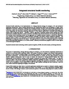
infer a single set of parameters θ, VB learning optimizes a whole ensemble over θ. The relevant update equations, specialized to the case of hidden Markov models, can be found in [11], [14], [15]. It is important to note that the computational complexity of variational Bayesian learning is not very different from that of the standard (maximum-likelihood) Baum-Welch algorithm [11], [14]. III. HMM BASED DAMAGE C LASSIFICATION A LGORITHM A. Time-Frequency Feature Extraction using MPD The critical first step of a successful classification system is the extraction of effective discriminatory features. In this work, we employ the amplitude-time-frequency-scale features {αk , τk , fk , κk } extracted by the MPD to encode the information necessary for distinguishing signals from different damage classes. Specifically, an L-iteration MPD is first applied to each measured signal, resulting in a collection of L continuous coefficients {αk , τk , fk , κk }k=0,...,L−1 . These are then cast as a sequence of 4-dimensional vectors of length T = L, and are subsequently used as a vector observation sequence to be statistically modeled for classification. B. Continuous HMM Based Damage Classifier The number of states N to use in the HMMs can be estimated empirically by examination of the TF representation of the data. Here we make use of the cross-term free TF representation given in [8] that can be computed directly from the signal MPD. We choose N using the number of stationarities in the data. An example of a 3-state definition is shown in Figure 1.
frequency (kHz)
250 200 150 100 50 0
Fig. 1.
1
2
3 4 time (sec)
assigns a given test observation sequence y� to damage class k, given by (j) k = arg max p(y� |θ ML , λN ), (9) j
(j) θML
where denotes the parameters of the jth HMM (trained on data from damage class j). C. Variational Bayes for Estimation of HMM State Number All other things being equal, the model complexity of the HMM is governed by the number of states N . The number of parameters to be estimated increases with N , and if the complexity of the model is not limited by the amount of data available, the result is overfitting. In this work, we use variational Bayes to select an HMM of appropriate complexity. Specifically, given data y, we employ the VB learning algorithm discussed in Section II-C to compute the evidence for the N -state HMM using H = λN in equation (7). The appropriate number of states N ∗ is then determined by comparing the evidences for various N as N ∗ = arg max p(y|λN ). N
(10)
VB learning provides an efficient framework for automatically selecting a model of appropriate complexity from the data, and helps avoid the overfitting problems encountered in conventional ML learning. IV. A PPLICATION E XAMPLES A. Experimental Setup and Data Collection The data comprises cyclic fatigue loading tests conducted on an Al 6061-T651 single-lap bolted joint sample. The experimental setup used is shown in Figure 2. The lap is 0.125 inches thick, with a 5 mm notch machined in the top lap. Nine piezoelectric sensors are mounted on the lap, one is used as an actuator for transmitting a 130 kHz burst signal and the remaining as receivers. Both structural and material damage is induced (separately) in the joint by subjecting it to a 20 Hz 90-900 kg tension-tension loading. Structural damage is defined here in terms of the torque on the bolts, and material damage based on the length of the crack initiated at the notch in response to fatiguing. Data is collected for four structural damage classes: bolt torque = 0%, 30%, 60%, and 100% (healthy), and eight material damage classes: number of fatigue cycles = 0 (healthy), 130, 135, 140, 145, 155, 200, and 285 kilo-cycles, with 100 measurements taken for each case. B. Choice of Model Parameters
5 −4
x 10
Example of a 3-state definition used in the HMM classifier.
The data from each damage class is modeled using an HMM, with the available training data from each class used to learn the parameters of the corresponding HMM. Once the model parameters have been estimated, unknown test data is classified based on its likelihood as computed by the HMM associated with each damage class. Specifically, the classifier
850
The measured signals are first mean-centered, normalized, and time-aligned. For each waveform, TF damage features are extracted using L = 20 MPD iterations with a dictionary composed of 5.8 million normalized time-frequency Gabor atoms given in (1). This choice of truncation limit corresponds to a residual signal energy of about 5%. For modeling with the discrete HMM, the features are quantized to K = 64, 128, and 256 symbols using the k-means algorithm [12]. In the continuous HMMs, M = 6 components are used with the Gaussian mixture models.
Fig. 2.
Setup for structural and material damage in a bolted joint.
Figure 3 shows an example plot of the log-evidence log p(y|λN ) (actually, the lower bound computed using VB learning) as a function of the number of HMM states N , for the case of structural damage with bolt at 60% torque. We see that the evidence is greatest for N = 2 to 5 state HMMs, and decreases as N is increased further (with increasing model complexity). In all the simulations of this paper, we use HMMs with N = 3 states. Note that this choice agrees well with the state definition shown in Figure 1, which was determined empirically.
as being from class j. In all cases, the correct classification probabilities (the diagonal entries of the confusion matrices) are highlighted with bold font. Tables I and II show the confusion matrices for structural damage classification using a discrete HMM with K = 256 symbols and a continuous HMM, respectively. While the K = 256-symbol discrete HMM classifier yields good classification results, the performance of the continuous HMM classifier is better (the average correct classification rate is higher). Table III shows the average correct classification rates for structural damage classification obtained from the discrete HMM (as a function of number of symbols used K) and the continuous HMM. We see that the performance of the discrete HMM classifier improves as K increases. This is expected, because the information loss associated with the quantization step is smaller for larger K. In addition, for all these choices of K, the performance of the continuous HMM classifier is superior to that of the discrete HMM classifiers. This improvement in performance from the discrete to the continuous HMM (and between discrete HMMs with increasing K) comes with added computational cost. 0.8667 0 0 0
0 0.9667 0.0333 0.0333
0.0667 0.0333 0.9333 0
0.0667 0 0.0333 0.9667
TABLE I S TRUCTURAL DAMAGE CLASSIFICATION USING DISCRETE HMM (K = 256 SYMBOLS ).
−3900
0.9667 0 0 0
−3950
log p(y|λN)
−4000
0 1.0000 0 0
0.0333 0 0.9333 0.0667
0 0 0.0667 0.9333
TABLE II S TRUCTURAL DAMAGE CLASSIFICATION USING CONTINUOUS HMM.
−4050
−4100
No. of symbols K Avg. correct classification rate
−4150
−4200 0
2
4 6 Number of HMM states (N)
8
64 0.8167
128 0.8583
256 0.9333
CHMM 0.9583
TABLE III S TRUCTURAL DAMAGE CLASSIFICATION RATES FROM DISCRETE HMM ( AS A FUNCTION OF K ) AND CONTINUOUS HMM (CHMM).
10
Fig. 3. Log-evidence log p(y|λN ) as a function of number of HMM states N , for the case of structural damage with bolt at 60% torque.
Of the 100 waveforms available for each damage class, 40 waveforms are used for training the HMMs, 30 are used for validation (estimating M for the continuous HMM), and 30 for testing classifier performance. C. Classification Results The performance of the classifier is quantified here using confusion matrices. The (i, j)th element of a confusion matrix indicates the probability that data from class i is classified
851
Tables IV and V show the confusion matrices for material damage classification using a discrete HMM with K = 256 symbols and a continuous HMM, respectively. Table VI shows the average correct classification rates for material damage classification obtained from the discrete HMM (as a function of number of symbols used K) and the continuous HMM. Once again, we see good classification results from both classifiers. And as before, the performance improves with K for the discrete HMM; the continuous HMM yields the best performance.
0.83 0 0 0 0 0 0 0
0 0.87 0.07 0 0 0 0 0.03
0 0 0.77 0 0 0.03 0 0
0.07 0 0 1.00 0 0 0 0.03
0 0.03 0 0 0.97 0 0 0
0.10 0.03 0 0 0.03 0.93 0.03 0.07
0 0.03 0 0 0 0 0.97 0
No. of symbols K Avg. correct classification rate
0 0.03 0.17 0 0 0.03 0 0.87
0 0.93 0 0 0 0 0 0
0 0 0.97 0 0 0 0 0
0 0 0 0.97 0 0 0 0
0 0 0 0 0.97 0 0 0
0 0.07 0.03 0.03 0.03 1.00 0.03 0.07
0 0 0 0 0 0 0.97 0
128 0.8030
256 0.9000
CHMM 0.9667
TABLE VI M ATERIAL DAMAGE CLASSIFICATION RATES FROM DISCRETE HMM ( AS A FUNCTION OF K ) AND CONTINUOUS HMM.
TABLE IV M ATERIAL DAMAGE CLASSIFICATION USING DISCRETE HMM (K = 256 SYMBOLS ).
1.00 0 0 0 0 0 0 0
64 0.7125
0 0 0 0 0 0 0 0.93
posterior over the parameters. Although we use a (maximumlikelihood) point estimate for the parameters, the approximate posterior can be applied for improved inference. Finally, in the results reported here, only data collected from one sensor was utilized. By fusing the information gathered from all of the multiple distributed sensors, the performance of the classifier can be improved significantly. ACKNOWLEDGMENT This research was supported by the DoD AFOSR Grant FA95550-06-1-0309 (Program manager: Victor Giurgiutiu). The authors would like to thank Clyde Coelho and Prof. Pedro Peralta for providing the experimental data used in this paper.
TABLE V M ATERIAL DAMAGE CLASSIFICATION USING CONTINUOUS HMM.
R EFERENCES V. C ONCLUSION We have presented an algorithm for the classification of structural damage based on time-frequency feature extraction and continuous hidden Markov models. Application to the detection of fatigue-induced structural and material damage in a bolted joint shows very good performance, and average correct classification rates of near 90% are observed. The performance of the discrete HMM classifier is a function of the number of symbols used, with more symbols yielding more accurate results. The performance of the continuous HMM classifier is superior to that of the discrete HMM classifier. The continuous HMM, however, is a more complex model and has more parameters to be estimated. As a result, the amount of data required for training the model can be greater. In addition, the number of mixture components to use in the Gaussian mixture models have to be determined using techniques such as cross-validation. Moreover, learning and inference in the continuous HMM is generally more computationally intensive than that for the discrete case. A variational Bayesian learning algorithm was applied to automatically select the number of states used in the HMM. This choice is shown to correlate well with what one might choose empirically by examination of the time-frequency features of the data in question. The HMM-based damage classification algorithm presented here can be enhanced in several ways. Firstly, by using the variational lower bound in place of the true evidence to guide model selection, we assumed that the KL divergences between the variational and exact posterior distributions over parameters and hidden variables are constant between models; this is not true in general. We are currently examining approaches to estimate the KL divergence. Second, the variational Bayesian learning yields not only a bound for the desired evidence but also an optimized variational approximation to the true
852
[1] B. C. Lee and W. J. Staszewski, “Modelling of Lamb waves for damage detection in metallic structures: Part I. Wave propagation,” Smart Mater. Struct., vol. 12, pp. 804–814, 2003. [2] L. Eren and M. J. Devaney, “Bearing damage detection via wavelet packet decomposition of the stator current,” IEEE Transactions on Instrumentation and Measurement, vol. 53-2, pp. 431–436, 2004. [3] G. Park, A. C. Rutherford, H. Sohn, and C. R. Farrar, “An outlier analysis framework for impedance-based structural health monitoring,” Journal of Sound and Vibration, vol. 286, pp. 229–250, 2005. [4] H. Sohn, D. W. Allen, K. Worden, and C. R. Farrar, “Structural damage classification using extreme value statistics,” Journal of Dynamic Systems, Measurement, and Control, vol. 127, pp. 125–132, 2005. [5] J. W. Lee, G. R. Kirikera, I. Kang, M. J. Schulz, and V. N. Shanov, “Structural health monitoring using continuous sensors and neural network analysis,” Smart Mater. Struct., vol. 15, pp. 1266–1274, 2006. [6] N. Kovvali, S. Das, D. Chakraborty, D. Cochran, A. PapandreouSuppapola, and A. Chattopadhyay, “Time-frequency based classification of structural damage,” 48th AIAA/ASME/ASCE/AHS/ASC Structures, Structural Dynamics, and Materials Conference 23 - 26 April 2007, Honolulu, Hawaii, AIAA 2007-2055. [7] L. R. Rabiner, “A tutorial on hidden Markov models and selected applications in speech recognition,” ser. Proceedings of the IEEE, vol. 77, 1989, pp. 257–286. [8] S. G. Mallat and Z. Zhang, “Matching pursuits with time-frequency dictionaries,” IEEE Transactions on Signal Processing, vol. 41, pp. 3397–3415, 1993. [9] P. R. Runkle, P. K. Bharadwaj, L. Couchman, and L. Carin, “Hidden markov models for multiaspect target classification,” IEEE Transactions on Signal Processing, vol. 47, pp. 2035–2040, 1999. [10] W. Zhou, N. Kovvali, A. Papandreou-Suppappola, D. Cochran, and A. Chattopadhyay, “Hidden Markov model based classification of structural damage,” Proc. of SPIE, vol. 6523, p. 652311, 2007. [11] M. J. Beal, “Variational algorithms for approximate Bayesian inference,” Ph.D. dissertation, Gatsby Computational Neuroscience Unit, University College London, 2003. [12] D. J. C. MacKay, Information Theory, Inference, and Learning Algorithms. Cambridge University Press, 2003. [13] A. Dempster, N. Laird, and D. Rubin, “Maximum likelihood from incomplete data via the EM algorithm,” Journal of the Royal Statistical Society, Series B, vol. 39, pp. 1–38, 1977. [14] D. J. C. MacKay, “Ensemble learning for hidden Markov models,” Cavendish Laboratory, University of Cambridge, Tech. Rep., 1997. [15] S. Ji, B. Krishnapuram, and L. Carin, “Variational Bayes for continuous hidden Markov models and its application to active learning,” IEEE Transactions on Pattern Analysis and Machine Intelligence, vol. 28, pp. 522–532, 2006.