Data augmentation for models based on rejection sampling

Data augmentation for models based on rejection sampling Vinayak Rao, Lizhen Lin, and David Dunson

arXiv:1406.6652v1 [stat.CO] 25 Jun 2014

Department of Statistical Science, Duke University, USA {VAR 11, LIZHEN , DUNSON}@ STAT. DUKE . EDU Editor:

Abstract We present a data augmentation scheme to perform Markov chain Monte Carlo inference for models where data generation involves a rejection sampling algorithm. Our idea is to instantiate the rejected proposals preceding each data point, and we show that this can be done easily and efficiently. The resulting joint probability over observed and rejected variables can be much simpler than the marginal distribution over the observed variables, which often involve intractable integrals. Our algorithm is an instance of a growing body of work on exact Markov chain Monte Carlo inference for doubly-intractable distributions and we consider two such problems. The first is a Bayesian analysis of the matrix Langevin distribution on the Stiefel manifold, and the second Bayesian inference for a nonparametric Gaussian process density model. Our experiments demonstrate superior performance over state-of-the-art sampling algorithms for such problems. Keywords: Bayesian inference; Density estimation; Doubly intractable; Gaussian process; Matrix Langevin; Markov Chain Monte Carlo; Rejection sampling; Stiefel manifold.

1. Introduction Rejection sampling allows us to sample from a probability density p(x) by constructing an upper bound to p(x), and accepting or rejecting samples from a density proportional to the bounding envelope. The envelope usually is much simpler than p(x), with the number of rejections, and thus the algorithm’s efficiency, determined by how closely it matches the true density. In typical applications, the probability density of interest is indexed by a parameter θ, and we write it as p(x | θ). A Bayesian analysis places a prior on θ, and given observations from the likelihood p(x | θ), studies the posterior over θ. An intractable likelihood, often with a normalization constant depending on θ, precludes straightforward Markov chain Monte Carlo inference over θ: calculating a Metropolis-Hastings acceptance ratio involves evaluating the ratio of two such likelihoods, and is itself intractable. This class of problems is called ‘doubly intractable’ (Murray et al., 2006), and existing approaches require the ability to draw exact samples from p(x | θ), or to obtain positive unbiased estimates of p(x | θ). 1

We describe a different approach that is applicable when p(x | θ) has an associated rejection sampling algorithm. Our idea is to instantiate the rejected proposals that preceded each observation, resulting in an augmented state-space on which we run a Markov chain. Including the rejected proposals as auxiliary variables eliminates any intractable terms, and allows the application of standard techniques. Importantly, we show that conditioned on the observations, it is straightforward to independently sample the number and values of the rejected proposals: this just requires running the rejection sampler to generate as many acceptances as there are observations, with all rejected proposals kept. The ability to produce a conditionally independent draw of these variables is important when posterior updates of some parameters are intractable, while others are simple. In such a situation, we introduce the rejected variables only when we need to carry out the intractable updates, after which we discard them and carry out the simpler updates.

2. Rejection sampling Consider a probability density p(x | θ) = f (x, θ)/Z(θ) on some space X, with the parameter θ taking values in Θ. We assume that the normalization constant Z(θ) is difficult to evaluate, so that na¨ıvely sampling from p(x | θ) is not easy. We also assume there exists a second, simpler density q(x | θ) ≥ f (x, θ)/M for all x, and for some positive M . Rejection sampling generates samples distributed as p(· | θ) by first proposing samples from q(· | θ). A draw y from q(· | θ) is accepted with probability f (y, θ)/ {M q(y | θ)}. Let there be r rejected proposals preceeding an accepted sample x, and denote them by Y = {y1 , · · · , yr } where r itself is a random variable. Write |Y| = r, so that the joint probability is       |Y| Y f (x, θ) f (y , θ) i  q(x | θ) p(Y, x) =  q(yi | θ) 1 − M q(y | θ) M q(x | θ) i i=1  |Y|  f (x, θ) Y f (yi , θ) = (q(yi | θ) − . M i=1 M

(1)

It is well known that this procedure recovers samples from p(x | θ), so that the expression above has the correct marginal distribution over x (Robert and Casella, 2005). Later, we will need to sample the rejected variables Y given an observation x drawn from p(· | θ). Simulating from p(Y | x, θ) involves the following two steps in Algorithm 1. Algorithm 1 relies on the following proposition about the conditional p(Y | x, θ). Proposition 1 The set of rejected samples Y preceding an accepted sample x is independent of x: p(Y | θ, x) = p(Y | θ). We can thus assign x the set Yb of another sample, xˆ. 2

Algorithm 1 Algorithm to sample from p(Y | x, θ) Input: A sample x, and the parameter value θ Output: The set of rejected proposals Y preceeding x 1: 2:

Draw sample yi independently from q(· | θ) until a point xˆ is accepted. Discard xˆ, and treat the preceeding rejected proposals as Y.

3. Bayesian Inference 3.1 Sampling by introducing rejected proposals of the rejection sampler Given observations X = {x1 , · · · , xn }, and a prior p(θ), Bayesian inference typically uses Markov chain Monte Carlo to sample from the intractable posterior p(θ | X). We partition θ into (θ1 , θ2 ) so that the normalization constant factors as Z(θ) = Z1 (θ1 )Z2 (θ2 ), with the first term Z1 simple to evaluate, and Z2 intractable. Consequently, updating θ1 with θ2 fixed is straightforward; in fact there are situations where we can place a conjugate prior on θ1 . Inference over θ2 is a doubly-intractable problem. We assume that p(x | θ) has an associated rejection sampling algorithm with proposal density q(x | θ) ≥ f (x, θ)/M . For the ith observation xi , write the preceding set of rejected samples as Yi = {yi1 , . . . , yi|Yi | }. The joint density of all samples, both rejected and accepted, is then P (x1 , Y1 , . . . , xn , Yn ) =

|Yi |  n Y f (xi , θ) Y i=1

M

j=1

f (yij , θ) q(yij | θ) − M

 .

This does not involve any intractable terms, so that standard techniques can be applied to update θ. To introduce the rejected proposals Yi , we simply follow Algorithm 1: draw proposals from q(· | θ) until we have n acceptances, with the ith batch of rejected proposals forming the set Yi . The ability to produce conditionally independent draws of Y is important when some components of θ have simple conditional posterior distributions. For instance, if there exists a conjugate prior p1 (θ1 ) on θ1 for the likelihood p(x | θ1 , θ2 ), then introducing the rejected proposals Yi breaks this conjugacy. The resulting complications in updating θ1 can slow down mixing of the Markov chain, especially when θ1 is high dimensional. A much cleaner solution is to sample θ1 from its conditional posterior p(θ1 | X, θ2 ), introducing the auxiliary variables only when needed to update θ2 . After updating θ2 , they can then be discarded. Algorithm 2 describes this. 3.2 Related work One of the simplest, and most widely applicable Markov chain Monte Carlo algorithms for doubly-intractable distributions is the exchange sampler of Murray et al. (2006). Simplifying an earlier idea by Møller et al. (2006), this algorithm effectively amounts to the 3

Algorithm 2 An iteration of the Markov chain for posterior inference over θ = (θ1 , θ2 ) Input: The observations X, and the current parameter values (θ1 , θ2 ) Output: New parameter values (θ˜1 , θ˜2 ) 1: 2: 3: 4:

|X|

Run Algorithm 1 |X| times, keeping all the rejected proposals Y = ∪i=1 Yi . Update θ˜2 with a Markov kernel having p(θ˜2 | X, Y, θ1 ) as stationary distribution. Discard the rejected proposals Y. Sample θ˜1 from its posterior p(θ1 | X, θ2 ).

following: given the current parameter θcurr , propose a new parameter θnew according to some proposal distribution. Additionally, generate a dataset of n ‘pseudo-observations’ {ˆ xi } from p(x | θnew ). The exchange algorithm then proposes swapping the parameters associated with datasets. Murray et al. (2006) show that all intractable terms cancel out in the resulting acceptance probability, and that the resulting Markov chain has the correct stationary distribution. While the exchange algorithm is applicable whenever one can sample from the likelihood p(x | θ), it does not exploit the mechanism used to produce these samples. When the latter is a rejection sampling algorithm, each pseudo-observation is preceeded by a sequence of rejected proposals. These are all discarded, and only the accepted proposals are used to evaluate the new parameter θnew . By contrast our algorithm explicitly instantiates these rejected proposals, so that they can be used to make good proposals. In our experiments, we use a Hamiltonian Monte Carlo sampler on the augmented space and exploit gradient information to make nonlocal moves with high probability of acceptance. For reasonable acceptance probabilities under the exchange sampler, one must make local updates to θ, or resort to complicated annealing schemes. Another framework for doubly intractable distributions is the pseudo-marginal approach of Andrieu and Roberts (2009). The idea here is that even if we cannot exactly evaluate the acceptance probability, it is sufficient to use a positive, unbiased estimate: this will still result in a Markov chain with the correct stationary distribution. In our case, instead of requiring an unbiased estimate, we require an upper bound M to the normalization constant Z(θ). Additionally, like the exchange sampler, the pseudo-marginal method provides a mechanism to evaluate a proposed parameter θnew ; how to make good proposals is less obvious. Related to our ideas is a sampler from Adams et al. (2009), see also Section 6. Their problem also involved inferences on the parameters governing the output of a rejection sampling algorithm. Like us, they proceeded by augmenting the state space to include the rejected proposals Y. However, rather than generating independent realizations of Y when needed, Adams et al. (2009) outlined a set of Markov transition operators to perturb the current configuration of Y, while maintaining the correct stationary distribution. With prespecified probabilities, they proposed adding a new variable to Y, deleting a variable from Y and perturbing the value of an existing element in Y. These local updates to Y 4

can slow down Markov chain mixing, require the user to specify a number of parameters, and also involve calculating Metropolis-Hastings acceptance probabilities for each local step. Furthermore, the Markov nature of their updates require them to maintain the rejected proposals at all times, complicating inferences over other parameters. Our algorithm is much simpler and cleaner.

4. Convergence properties Write the Markov transition density of our chain as k(θˆ | θ), and the m-fold transition density as k m (θˆ | θ). For simplicity, we suppress the fact that these depend on the data X. The Markov chain is said to be uniformly ergodic if there exist constants C and ρ such that for all m and θ, Z |p(θˆ | X) − k m (θˆ | θ)|dθ ≤ Cρm . Θ

The term to the left is twice the total variation distance between the desired posterior and the state of the Markov chain initialized at θ after m iterations. Small values of ρ imply faster mixing. The following minorization condition is sufficient for uniform ergodicity (Jones and ˆ and a δ > 0 such that for all θ, θˆ ∈ Θ, Hobert, 2001): there exists a probability density h(θ) ˆ k(θˆ | θ) ≥ δh(θ).

(2)

When this holds, the mixing rate ρ ≤ 1 − δ, so that a large δ implies rapid mixing. Our Markov transition density first introduces the rejected proposals Y, and then conditionally updates θ. The set Yi preceeding the ith observation takes values in the union r space U ≡ ∪∞ r=0 X . The output of the rejection sampler, including the ith observation, lies in the product space U×X with density given by equation (1), so that any (Y, x) ∈ (U×X) has probability  |Y|  Y f (yi , θ) f (x, θ) λ(dx) q(yi | θ) − λ(dyi ). p(Y, x | θ) = M M i=1 Here, λ is the measure with respect to which the densities f and q are defined, and it is easy to see that the above quantity integrates to 1. From Bayes’ rule, the conditional density over Y is  |Y|  1 Y f (yi , θ) q(yi | θ) − p(Y | x, θ) = λ(dyi ). M i=1 M The fact that the right hand side does not depend on x is an alternate proof of Proposition 1. This density characterizes the data augmentation step of our sampling algorithm. In practice, we need as many draws from this density as there are observations. 5

The second step of sampling from p(θˆ | Y, X, θ) depends on the problem at hand. We simplify matters by assuming we can sample from p(θˆ | Y, X) independently of the old θ: this is the classical data augmentation algorithm. We also assume that the proposal density q(· | θ) is uniformly bounded from above and below by finite, positive quantities B and b, and that the probability of rejection for the rejection sampler is bounded below by a positive r. Letting β = br/B, we can easily verify that p(θˆ | Y, X) ≥ β |Y| p(θˆ | X). We can now state our result. Theorem 2 Assume that the proposal density q(x | θ) has uniform lower and upper bounds b and B, and the probability of rejection is bounded below by r, with r, b > 0. Further assume we can sample from the conditional p(θˆ | Y, X). Then our hdata augmentation i 1 algorithm is uniformly ergodic with mixing rate ρ upper bounded by 1 − {M (1−β)−β} n , where β = br/B. Despite our simplifying assumptions, our theorem has a number of useful implications. Firstly, the smaller M is, the lower the bound is, suggesting faster mixing. Recall that M is a measure of how well our proposal distribution q(· | θ) matches the distribution of interest f (· | θ). The theorem suggests that the closer the match, the faster the chain mixes. This makes intuitive sense: a poor proposal density will result in more rejected proposals Y, and will increase the coupling between successive θ’s in the Markov chain. The parameter r has a similar effect. Also, the larger the number of observations n is, the more slowly the chain mixes. Again, from the construction of our chain this makes sense. We suspect this property holds for most exact samplers for doubly-intractable distributions, though we are unaware of any such result. Even without assuming we can sample from p(θˆ | Y, X), our ability to sample Y independently means that the marginal chain over θ is still Markovian. By contrast, existing approaches (Adams et al. (2009); Walker (2011)) only produce dependent updates in the complicated auxiliary space: they sample from p(Yˆ | θ, Y, X) by making local updates to Y. Consequently, these chains are Markovian only in the complicated augmented space, and the marginal processes over θ have long-term dependencies. Besides affecting mixing, this can also complicate analysis. In the following sections we apply our sampling algorithm to two problems, one involving Bayesian inference for the matrix Langevin distribution, and the second, the Gaussian process density sampler of Adams et al. (2009).

5. Bayesian inference for the matrix Langevin distribution 5.1 The Matrix Langevin distribution on the Stiefel manifold The Stiefel manifold Vp,d is the space of all d × p orthonormal matrices, that is, d × p matrices X such that X T X = Ip where Ip is the p × p identity matrix. When p = 1, this is the d − 1 hypersphere S d−1 , and when p = d, this is the space of all the orthonormal matrices O(d). Probability distributions on the Stiefel manifold play an important role 6

in statistics, signal processing and machine learning, with applications ranging from studies of orientations of orbits of comets and asteroids to principal components analysis to the estimation of rotation matrices. The simplest such distribution is the matrix Langevin distribution, an exponential-family distribution whose density with respect to the invariant Haar volume measure (Edelman et al., 1998) is pML (X | F ) = etr(F T X)/Z(F ). Here etr is the exponential-trace, and F is a d × p matrix. The normalization constant Z(F ) = 0 F1 ( 21 d, 14 F T F ) is the hypergeometric function with matrix arguments, evaluated at 14 F T F (Chikuse, 2003). Let F = GκH T be the singular value decomposition of F , where G and H are d × p and p × p orthonormal matrices, and κ is a positive diagonal matrix. We parametrize pML by (G, κ, H), and one can think of G and H as orientations, with κ controlling the concentration in directions determined by these orientations. Large values of κ imply concentration along the associated directions, while setting κ to zero gives the uniform distribution on the Stiefel manifold. It can be shown (Khatri and Mardia, 1977) that 0 F1 ( 21 d, 14 F T F ) = 0 F1 ( 21 d, 14 κT κ), so that this depends only on κ. We write it as Z(κ).

In our Bayesian analysis, we place independent priors on κ, G and H. The latter two lie on the Stiefel manifolds Vp,d and Vp,p , and we place matrix Langevin priors pML (· | F0 ) and pML (· | F1 ) on these: we will see below that these are conditionally conjugate. We place independent Gamma(a0 , b0 ) priors on the diagonal elements of κ. However, the difficulty in evaluating the normalization constant Z(κ) makes posterior inference over κ doubly intractable. Thus, in a 2006 University of Iowa PhD thesis, Camano-Garcia keeps κ constant, while Hoff (2009b) uses a first-order Taylor expansion of the intractable term to run an approximate sampling algorithm. Below, we show how fully Bayesian inference can be carried out over this quantity as well.

5.2 A rejection sampling algorithm

We first describe a rejection sampling algorithm from Hoff (2009a) to sample from pML . For simplicity, assume H is the identity matrix. In the general case, we simply rotate the resulting draw by H, since if X ∼ pML (· | F ), then XH ∼ pML (· | F H T ). At a high level, the algorithm sequentially proposes vectors from the matrix Langevin on the unit sphere: this is also called von Mises-Fisher distribution and is easy to simulate (Wood, 1994). The mean of the rth vector is column r of G, G[:r] , projected onto the nullspace of the earlier vectors, Nr . This sampled vector is then projected back onto Nr and normalized, and the process is repeated p times. Call the resulting distribution pseq ; for more details, see Algorithm 3 and Hoff (2009a). 7

Algorithm 3 Proposal distribution pseq (· | G, κ) for matrix Langevin distribution (Hoff, 2009a) Input: Parameters G, κ; write G[:i] for column i of G, and κi for element (i, i) of κ Output: An output X ∈ Vp,d ; write X[:i] for column i of X 1:

Sample X[:1] ∼ pML (· | κ1 G[:1] ). For r ∈ {2, · · · p} (a) Construct Nr , an orthogonal basis for the nullspace of {X[:1] , · · · X[:r−1] }. (b) Sample z ∼ pML (· | κr NrT G[:r] ), and (c) Set X[:r] = z T Nr /kz T Nr k.

It can be seen that pseq is a density on the Stiefel manifold taking the form ( p ) Y kκr NrT G[:r] /2k(d−r−1)/2 pseq (X | G, κ) = etr(κGT X), d−r+1 T Γ( 2 )I(d−r−1)/2 (kκr Nr G[:r] k) r=1

(3)

where Ik (·) is the modified Bessel function of the first kind. Write D(X, κ, G) for the reciprocal of the term in braces. Since Ik (x)/xk is an increasing function of x, and kNrT G[:r] k ≤ kG[:r] k = 1, we have the following bound D(κ) for D(X, κ, G): D(X, κ, G) ≤

p Y Γ( d−r+1 )I(d−r−1)/2 (kκr k) 2

r=1

kκr /2k(d−r−1)/2

= D(κ)

This implies etr(κGT X) ≤ D(κ)pseq (X | G, κ), allowing the following rejection sampler: draw a sample X from pseq (·), and accept with probability D(X, κ, G)/D(κ). The accepted proposals come from pML (· | G, κ), and for samples from pML (· | G, κ, H), postmultiply these by H. 5.3 Posterior sampling Given a set of n observations {Xi }, and writing S =

Pn

i=1

Xi , we have:

p(G, κ, H | Xi }) ∝ etr(HκGT S)p(H)p(G)p(κ)/Z(κ)n . At a high level, our approach is a Gibbs sampler that sequentially updates H, G and κ. The first two steps are straightforward, while the third will require our data augmentation scheme. 1. Updating G and H: With a matrix Langevin prior on H, the posterior is  p(H | Xi }, κ, G) ∝ etr (S T Gκ + F0 )T H . 8

This is just the matrix Langevin distribution over rotation matrices, and one can sample from this following Section 5.2. From here onwards, we will rotate the observations by H, allowing us to ignore this term. Redefining S as SH, the posterior over G is also a matrix Langevin:  p(G | Xi }, κ) ∝ etr (Sκ + F1 )T G . 2. Updating κ: Here, we exploit the rejection sampler scheme of the previous section, and instantiate the rejected proposals using Algorithm 1. From Section 5.2, the joint probability is  n P i | o |Y| n Y etr κGT S + |Y Y j=1 Yij {D(κ) − D(Yij , G, κ)} p({Xi , Yi } | G, κ) = . (4) D(κ)1+|Y| D(Y , G, κ) ij i=1 j=1 All terms in the expression above can be evaluated easily, allowing a simple MetropolisHastings algorithm in this augmented space. In fact, we can go further, calculating gradients to run a Hamiltonian Monte Carlo algorithm (Neal, 2010) that makes significantly more sampling algorithm. In particular, let N = n+ P|Yi | Pn than a random-walk Pn efficient proposals j=1 Yij ). The log joint probability L ≡ log {p({Xi , Yi })} i=1 (Xi + i=1 |Yi |, and S = is T

L = trace(G κS) +

|Yi | n X X

[log {D(κ) − D(Yij , κ)} − log{D(Yij , κ)}] − n log {D(κ)} .

i=1 j=1

n Q Writing D(Y, κ) = C pr=1 dL = GT[,k] S[,k] + dκk

i=1

o

˜ as C D(Y, κ), Appendix B shows that

 I(d−k+1)/2 T T (κ ) − N G (κ N G ) k k k k k k I I(d−k−1)/2  I(d−k−1)/2  − N (d−k+1)/2 (κk ). o n ˜ ij ,κ) D(Y I(d−k−1)/2 1 − D(κ) j=1 ˜

|Yi | n X X

I

I(d−r−1)/2 (kκr NrT Gr k) kκr NrT Gr k(d−r−1)/2 (d−k+1)/2

We use this gradient information to construct a Hamiltonian Markov chain Monte Carlo algorithm (Neal, 2010) that explores κ-space. For our purposes, it suffices to note that a proposal of this sampler involves taking L ‘leapfrog’ steps of size  along the gradient, and then accepting the resulting state with probability proportional to the product of equation (4), and a simple Gaussian ‘momentum’ term. The acceptance probability depends on how accurately the -discretization approximates the continuous dynamics of the system, and choosing a small  and a large L can give global moves with high acceptance probability. On the other hand, a large L comes at the cost of a large number of gradient evaluations. We study this trade-off in Section 5.5. 5.4 Vectorcardiogram dataset The vectorcardiogram is a loop traced by the cardiac vector during a cycle of the heart beat. The two directions of orientation of this loop in three-dimensions form a point on the Stiefel 9

Posterior probability

1.0

0.5 0.5

0.0

0.5

1.0

1.0

Posterior probability

0.0

0.2 0.15 0.1 0.05 0

0.5 1.0 0.5 0.0 0.5 1.0 1.0

0.25

4

6

8

10

8 κ1

10

12

0.2 0.15 0.1 0.05 0

12

14

16

18

κ1

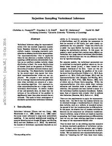
Figure 1: (Left) Vector cardiogram dataset with inferences. Bold lines are maximum likelihood estimates of G, and solid circles contain 90% posterior mass. Dashed circles are 90% predictive probability regions. (Right) Posterior over κ1 and κ2 , circles are maximum likelihood estimates.

manifold. The dataset of Downs et al. (1971) includes 98 such recordings, and is displayed in the left subplot of Figure 1. We represent each observation with a pair of orthonormal vectors, with the set of cyan lines to the right forming the first component. This empirical distribution possesses a single mode, so that the matrix Langevin distribution appears a suitable model. We place independent uninformative exponential priors with mean 10 and variance 100 on the scale parameter κ, and a uniform prior on the location parameter G. We restrict H to be the identity matrix. Inferences were carried out using the Hamiltonian sampler to produce 10000 samples, with a burn-in period of 1000. For the leapfrog dynamics, we set a step size of 0.3, with the number of steps equal to 5. We fix the ‘mass parameter’ to the identity matrix as is typical. We implemented all algorithms in R, building on code from the rstiefel package of Peter Hoff. All simulations were run on an Intel Core 2 Duo 3 Ghz CPU. For comparison, we include the maximum likelihood estimates of κ and G. For κ1 and κ2 , these were 11.9 and 5.9, and we plot these in the right half of Figure 1 as the red circles. The bold straight lines in Figure 1(left) show the maximum likelihood estimates of the components of G, with the small circles corresponding to 90% Bayesian credible regions estimated from the Monte Carlo output. The dashed circles correspond to 90% predictive probability regions for the Bayesian model. For these, we generated 50 points on V3,2 for each sample, with parameters specified by that sample. The dashed circles contain 90% of these points across all samples. Figure 1(right) show the posterior over κ1 and κ2 . 10

Effective samples per second 1 2 3 4 0

Effective samples per second 0.1 0.3 0.5 0.7 0 0.1

0.3 0.5 1 1.5 2 Variance of Metropolis proposals

0.1

0.3 0.5 random Leapfrog step size

Figure 2: Effective samples per second for (left) random walk and (right) Hamiltonian samplers. From bottom to top at abscissa 0.5: (left) Metropolis-Hastings data-augmentation sampler and exchange sampler, and (right) 1/10/5/3 leapfrog steps of Hamiltonian sampler. 5.5 Comparison of exact samplers To quantify sampler efficiency, we estimate the effective sample sizes produced per unit time. This corrects for correlation between successive Markov chain samples by estimating the number of independent samples produced; for this we used the rcoda package of Plummer et al. (2006). The left plot in Figure 2 considers two Metropolis-Hastings samplers, the exchange sampler and our latent variable sampler on the vectorcardiogram dataset. Both samplers perform a random walk in the κ-space, with the steps drawn for a normal distribution whose variance increases along the horizontal axis. The vertical axis shows the median effective sample size per second for the components of κ. The figure shows that both samplers’ performance peaks when the proposals have a variance between 1 and 1.5, with the exchange sampler performing slightly better. However, the real advantage of our sampler is that introducing the latent variables results in a joint distribution without any intractable terms, allowing the use of more sophisticated sampling algorithms. The plot to the right studies the Hamiltonian Monte Carlo sampler described at the end of Section 3.1. Here we vary the size of the leapfrog steps along the horizontal axis, with the different curves corresponding to different numbers of leapfrog steps. We see that this performs an order of magnitude better than either of the previous algorithms, with performance peaking with 3 to 5 steps of size 0.3 to 0.5, fairly typical values for this algorithm. This shows the advantage of exploiting gradient information in exploring the parameter space. 5.6 Comparison with an approximate sampler In this section, we consider an approximate sampler based on an asymptotic approximation to Z(κ) = 0 F1 ( 21 d, 14 κT κ) for large values of (κ1 , · · · , κn ) (Khatri and Mardia, 1977): ( Z(κ) '

1

1

2− 4 p(p+5)+ 2 pd 1

π 2p

)

) p #−1   "(Y p p j−1 Y Y Y 1 (d−p) 1 d−j+1 etr(κ) Γ κi2 . (κi + κj ) 2 2 j=1 j=2 i=1 i=1 11

2

2

0 −1

−1

0

0

1

Error in

Error in

1

2 1

Error in

−1 3

4

5

8

10

Ambient dimensionality

3

4

5

8

10

Ambient dimensionality

3

4

5

8

10

Ambient dimensionality

Figure 3: Errors in the posterior mean. Solid/dashed lines are Hamiltonian/approximate sampler.

We use this approximation in the acceptance probability of a Metropolis-Hastings algorithm; it can similarly be used to construct a Hamiltonian sampler. Such approximate schemes involve the ratio of two approximations, and can have very unpredictable performance. On the vectorcardiogram dataset, the approximate sampler based on the asymptotic expansion is about forty times faster than the exact samplers. For larger datasets, this difference will be even greater, and the real question is how accurate the approximation is. Our exact sampler allows us to study this: we consider the Stiefel manifold Vd,3 , with the three diagonal elements of κ set to 1, 5 and 10. With this setting of κ, and a random G, we generate datasets with 50 observations with d taking values 3, 4, 5, 8, and 10. In each case, we estimate the posterior mean of κ by running the exchange sampler, and treat this as the truth. We compare this with posterior means returned by our Hamiltonian sampler, as well as the approximate sampler. Figure 3 shows these results, with the three subplots corresponding to the three components of κ, and ambient dimensionality d increasing along the horizontal axis. As expected, the two exact samplers agree, and the Hamiltonian sampler has almost no ‘error’. The approximate sampler is more complicated. For values of d around 5, its estimated posterior mean is close to that of the exact samplers. Smaller values lead to an approximate posterior mean that underestimates the actual posterior mean, while in higher dimensions, the opposite occurs. Recalling that κ controls the concentration of the matrix Langevin distribution about its mode, this implies that in high dimensions, the approximate sampler will underestimate uncertainty in the distribution of future observations.

6. The Gaussian process density sampler Our next application is the Gaussian process density sampler of Adams et al. (2009), a nonparametric prior for a probability density induced by a logistic transformation of a random function from a Gaussian process. Letting σ(·) denote the logistic function, the random 12

density is g(x) ∝ g0 (x)σ{f (x)},

f ∼ GP,

with g0 (·) a parametric base density and GP denoting a Gaussian process. The inequality g0 (x)σ{f (x)} ≤ g0 (x) allows a rejection sampling algorithm by making proposals from g0 (·). At a proposed location x∗ , we sample the function value f (x∗ ) conditioning on all previous evaluations, and accept the proposal with probability σ{f (x∗ )}. Such a scheme involves no approximation error, and only requires evaluating the random function on a finite set of points. Algorithm 4 describes the steps involved in generating n observations. Algorithm 4 Generate n new samples from the Gaussian process density sampler Input: A base probability density g0 (·), ˜ and Y˜ , Previous accepted and rejected proposals X Gaussian process evaluations fX˜ and fY˜ at these locations. Output: n new samples X, with the associated rejected proposals Y , Gaussian process evaluations fX and fY at these locations. 1: 2: 3:

repeat Sample a proposal y from g0 (·). Sample fy , the Gaussian process evaluated at y, conditioning on fX , fY , fX˜ and fY˜ .

4: 5: 6: 7: 8: 9:

with probability σ(fy ) Accept y and add it to X. Add fy to fX . else Reject y and add it to Y . Add fy to fY . end until n samples are accepted.

6.1 Posterior inference Given observations X = {x1 , · · · , xn }, we are interested in p(g | X), the posterior over the underlying density. Since g is determined by the modulating function f , we focus on p(f | X). While this quantity is doubly intractable, after augmenting the state space to include the proposals Y from the rejection sampling algorithm, p(f | X, Y) has density Q Q with respect to the Gaussian process prior given by ni=1 σ {f (xi )} |Y| i=1 [1 − σ {f (yi )}], see also Adams et al. (2009). In words, the posterior over f evaluated at X ∪ Y is just the posterior from a Gaussian process classification problem with a logistic link-function, and with the accepted and rejected proposals corresponding to the two classes. There are a number of Markov chain Monte Carlo methods such as Hamiltonian Monte Carlo or elliptical slice sampling (Murray et al., 2010) that are applicable in such a situation. Given f on X∪Y, it can be evaluated anywhere else by conditionally sampling from a multivariate normal. 13

Modulating intensity

Probability density

6

0.8 0.6 0.4 0.2 0 −2−1 0 1 2 3 4 5 6 7 8 9 101112 Normalized velocity

4 2 0 −2 −4 −6 −2−1 0 1 2 3 4 5 6 7 8 9 101112 Normalized velocity

Figure 4: (Left) Posterior density for the galaxy dataset and (Right) Posterior over the Gaussian process function. Both plots show the median with 80 percent posterior credible intervals.

Sampling the rejected proposals Y given X and f is straightforward by Algorithm 1: run the rejection sampler until n accepts, and treat the rejected proposals generated along the way as Y. In practice, we do not have access to the entire function f , only its values evaluated on X and Yold , the location of the previous thinned variables. However, just as under the generative mechanism, we can retrospectively evaluate the function f where needed. After proposing from g0 (·), we sample the value of the function at this location conditioned on all previous evaluations, and use this value to decide whether to accept or reject. We outline the inference algorithm in Algorithm 5, noting that it is much simpler than that proposed in Adams et al. (2009). We also refer to that paper for limitations of the exchange sampler in this problem.

Algorithm 5 A Markov chain iteration for inference in the Gaussian process density sampler Input: Observations X with corresponding function evaluations f˜X , Current rejected proposals Y˜ with corresponding function evaluations f˜Y˜ . Output: New rejected proposals Y , New Gaussian process evaluations fX and fY at X and Y , New hyperparameters. Run Algorithm 4 to produce |X| accepted samples, with X, Y˜ , f˜X and f˜Y˜ as inputs. ˜ and f ˜ with values returned by the previous step; call these Y and fˆY . 2: Replace Y Y 3: Update f˜X and fˆY using for example, hybrid Monte Carlo, to get fX and fY . 4: Update parameters of the base-distribution, as well as the Gaussian process hyperparameters.

1:

14

0.2 Probability

Density of rejections

0.25

0.3

0.2

0.1

0.15 0.1 0.05

0 −2−1 0 1 2 3 4 5 6 7 8 9 101112 Normalized velocity

0

0

200 400 Number of rejections

600

Figure 5: (Left) Kernel density estimate of the locations of the rejected proposals and (Right) Histogram of the number of rejected proposals in each Markov chain iteration.

6.2 Experiments We consider the galaxy dataset from Postman et al. (1986), consisting of recorded velocities of 82 galaxies in the Corona Borealis. We normalized these to vary from 0 to 10. We used the model of Adams et al. (2009) as a prior on the underlying probability density, setting g0 (·) to a normal N (µ, σ 2 ), with a normal-inverse-Gamma prior on (µ, σ). The latter had parameters (0, .1, 1, 10). The Gaussian process had a squared-exponential kernel, with variance and length-scale of 1. We ran a Matlab implementation of our data augmentation algorithm to produce 2000 posterior samples after a burn-in of 500 samples. The Figure 4(left) shows the resulting posterior over the underlying density. This is clearly multimodal and non-Gaussian, with the modulating function allowing low-probability areas around either side of the main cluster of observations. The right bump away from the origin is slightly thinner that the left one because we have fewer observations there, but also since we centered our model around the origin. The right plot in the same figure focuses on the deviation from normality by plotting the posterior over the latent function. Inside the interval [0, 10], there are two dips in the Gaussian process intensity at [1, 3] and [7, 9], while over [3, 7], it is larger than its prior mean of 0. Figure 5 studies the distribution of the rejected proposals Y. The left plot shows the distribution of their locations: most of these occured in the low probability intervals [1, 3] and [7, 9]. The right plot is a histogram of the number of rejected proposals: this is typically around 100 to 200, though the largest value we observed was 611. Since inference over the latent function involves evaluating it at the locations of the accepted as well as rejected proposals, the largest covariance matrix we had to deal with was about 600 × 600; typical values were around 200 × 200. Using the same setup as Section 5.5, it took a na¨ıve Matlab implementation 11 minutes to run 2500 iterations. One can imagine computations becoming unwieldy for a large number of observations, or when there is large mismatch between the true density and the base-measure g0 (·). In such situations, one might have to choose the Gaussian process covariance kernel more carefully, use one of many sparse approximation techniques, or use other nonparametric priors like splines instead. In all 15

these cases, we can use our algorithm to recover the rejected proposals Y, and given these, posterior inference over f can be carried out using standard techniques.

7. Discussion We described a simple approach to carry out Markov chain Monte Carlo inference when data generation involves a rejection sampling algorithm. Our algorithm is simple and efficient, and allows us to exploit ideas like Hamiltonian Monte Carlo to carry out efficient inference. While our algorithm is exact, it also provides a framework for faster, approximate algorithms. For instance, the number of rejected proposals preceeding any observation is a random number that apriori is unbounded. One can bound the computational cost of an iteration by limiting the maximum number of rejected proposals. Similarly, one might try sharing rejected proposals across observations. We leave the study of the resulting Markov chain algorithms for future research. Also left open is a more careful analysis of Markov mixing rates for the applications we considered.

8. Acknowledgement This work was supported by the National Institute of Environmental Health Sciences of the National Institute of Health.

Appendix A. Proofs Proof [of Proposition 1] The probability density of an accepted sample x is p(x | θ) = f (x, θ)/Z(θ). Independently introduce the set (Y, xˆ) by running the rejection sampler until acceptance, so that 

  |Y|  Y x, θ) f (yi , θ)  f (x, θ)  f (ˆ q(yi | θ) − p(x, Y, xˆ | θ) = Z(θ) M i=1 M    |Y|  f (ˆ x, θ)  f (x, θ) Y f (yi , θ)  = (q(yi | θ) − . Z(θ) M i=1 M o Q|Y| n f (yi ,θ) Marginalizing out xˆ, we have p(Y, x) = f (x,θ) q(y | θ) − . i i=1 M M From equation (1), we see this is the desired joint distribution, proving our scheme is correct.

16

Proof [of Theorem 2] Let the number of observations |X| be n. Then, Z ˆ k(θ | θ) = p(θˆ | Y, X)p(Y | θ, X)dY Un

≥ p(θˆ | X)

n Z Y U

i=1

= p(θˆ | X)

n Z Y i=1

β |Yi | p(Yi | θ, X)dYi

β

|Yi |

U

 |Yi |  1 Y f (yji , θ) q(yji | θ) − λ(dyji ) M j=1 M

 |Yi |  n ∞ p(θˆ | X) Y X |Yi | Y 1 = β 1− M n i=1 M j=1 |Yi |=0

=

p(θˆ | X) Mn

n Y i=1

1 δ˜

δ˜ = 1 − β(1 − 1/M )

1 = M − β(M − 1) = M (1 − β) − β δn ˆ the posterior Thus k(θˆ | θ) satisfies equation (2), with δ n = 1/ [M {1 − β) − β}], and h(θ), ˆ p(θ | X). = δp(θˆ | X)

Appendix B. Gradient information For n pairs {Xi , Yi }, with N = n + T

Pn

log {P ({Xi , Yi })} = trace(G κS) +

i=1

|Yi |, and S =

|Yi | n X X

Pn

i=1 (Xi

+

P|Yi |

j=1

Yij ), we have

[log {D(κ) − D(Yij , κ)} − log {D(Yij , κ)}] − N log {D(κ)}

i=1 j=1

n Q Write D(Y, κ) = C pr=1

I(d−r−1)/2 (kκr NrT Gr k) kκr NrT Gr k(d−r−1)/2

o

d ˜ as C D(Y, κ). Since dx

˜ I(d−j+1)/2 dD(Y, κ) ˜ = NjT Gj D(Y, κ) (κj NjT Gj ) dκj I(d−j−1)/2

and

n

Im (x) xm

o

= x−m Im+1 (x),

˜ I(d−j+1)/2 dD(κ) ˜ = D(κ) (κj ). dκj I(d−j−1)/2

Then, writing L = log {P ({Xi , Yi })}, we have ( ) |Yi | n X X ˜ 0 (κ) ˜ 0 (κ) − D ˜ 0 (Yij , κ) D ˜ 0 (Yij , κ) D D dL = GT[,k] S[,k] + − −N ˜ ˜ ij , κ) ˜ ij , κ) ˜ dκk D(κ) − D(Y D(Y D(κ) i=1 j=1  I  |Yi |  (d−k+1)/2 (κ ) − N T G I(d−k+1)/2 (κ N T G )  n X X k kI k k k k I(d−k+1)/2 I(d−k−1)/2 (d−k−1)/2 T = G[,k] S[,k] + ( −N (κk ) ˜ D(Yij ,κ)   I (d−k−1)/2 1 − i=1 j=1 ˜ D(κ)

17

References Ryan Prescott Adams, Iain Murray, and David J. C. MacKay. The Gaussian process density sampler. In D. Koller, D. Schuurmans, Y. Bengio, and L. Bottou, editors, Adv. Neural Inf. Process. Syst. 21, pages 9–16. MIT Press, 2009. Christophe Andrieu and Gareth O. Roberts. The pseudo-marginal approach for efficient Monte Carlo computations. Ann. Stat., 37(2):697–725, April 2009. ISSN 0090-5364. doi: 10.1214/07-AOS574. URL http://dx.doi.org/10.1214/07-AOS574. Y. Chikuse. Statistics on Special Manifolds. Springer, New York, 2003. T. Downs, J. Liebman, and W. Mackay. Statistical methods for vectorcardiogram orientations. In Vectorcardiography 2: Proc. XIth Intn. Symp. Vectorcardiography (I. Hoffman, R.I. Hamby and E. Glassman, Eds.), pages 216–222, 1971. North-Holland, Amsterdam. A. Edelman, T.A. Arias, and S. T. Smith. The geometry of algorithms with orthogonality constraints. SIAM J. Matrix Anal. Appl, 20(2):303–353, 1998. P. D. Hoff. Simulation of the Matrix Bingham-von Mises-Fisher Distribution, with Applications to Multivariate and Relational Data. J. Comp. Graph. Stat., 18(2):438–456, 2009a. P. D. Hoff. A hiearchical eigenmodel for pooled covariance estimation. J. R. Statist. Soc. B, 71(5):971–992, 2009b. Galin L. Jones and James P. Hobert. Honest Exploration of Intractable Probability Distributions via Markov Chain Monte Carlo. Statist. Sci., 16(4):312–334, 11 2001. doi: 10. 1214/ss/1015346317. URL http://dx.doi.org/10.1214/ss/1015346317. C. G. Khatri and K. V. Mardia. The Von Mises-Fisher Matrix Distribution in Orientation Statistics. J. R. Statist. Soc. B, 39(1), 1977. ISSN 00359246. doi: 10.2307/2984884. URL http://dx.doi.org/10.2307/2984884. J. Møller, A. N. Pettitt, R. Reeves, and K. K. Berthelsen. An efficient Markov chain Monte Carlo method for distributions with intractable normalising constants. Biometrika, 93(2):451–458, 2006. doi: 10.1093/biomet/93.2.451. URL http://biomet. oxfordjournals.org/content/93/2/451.abstract. Iain Murray, Zoubin Ghahramani, and David J. C. MacKay. MCMC for doubly-intractable distributions. In Proc. 22nd Conf. Uncert. Artif. Intell., pages 359–366. AUAI Press, 2006. Iain Murray, Ryan Prescott Adams, and David J.C. MacKay. Elliptical slice sampling. J. Mach. Learn. Res. W&CP, 9, 2010. 18

Radford M. Neal. MCMC using Hamiltonian dynamics. Handbook of Markov Chain Monte Carlo, 54:113–162, 2010. Martyn Plummer, Nicky Best, Kate Cowles, and Karen Vines. CODA: Convergence diagnosis and output analysis for MCMC. R News, 6(1):7–11, March 2006. URL http://CRAN.R-project.org/doc/Rnews/. M. Postman, J. Huchra, and M. Geller. Probes of large-scale structure in the Corona Borealis region. Astron. J., 92:1238–1247, 1986. Christian P. Robert and George Casella. Monte Carlo Statistical Methods (Springer Texts in Statistics). Springer-Verlag New York, Inc., Secaucus, NJ, USA, 2005. ISBN 0387212396. Stephen G. Walker. Posterior sampling when the normalizing constant is unknown. Commun. Stat. Simulat., 40(5):784–792, 2011. doi: 10.1080/03610918. 2011.555042. URL http://www.tandfonline.com/doi/abs/10.1080/ 03610918.2011.555042. Andrew T.A. Wood. Simulation of the von Mises Fisher distribution. Commun. Stat. Simulat., 23(1):157–164, 1994. ISSN 0361-0918.

19