Data Center Optimization Methodology to Maximize ...

Data Center Optimization Methodology to Maximize the Usage of Locally Produced Renewable Energy Tudor Cioara, Ionut Anghel, Marcel Antal, Sebastian Crisan, Ioan Salomie Computer Science Department Technical University of Cluj-Napoca Cluj-Napoca, Romania {tudor.cioara, ionut.anghel, marcel.antal, sebastian.crisan, ioan.salomie}@cs.utcluj.ro Abstract — In this paper we address the problem of Data Centers energy efficiency by proposing a methodology which aims at planning the Data Center operation such that the usage of locally produced renewable energy is maximized. The methodology is based on an energy consumption flexibility mechanism that is defined for different types of Data Center components (electrical cooling system, IT workload, energy storage and diesel generators). The flexibility mechanism enacts the possibility of shifting the Data Center energy demand from time intervals with limited renewable energy production due to weather conditions, to time intervals when spikes of renewable energy production are predicted. We have developed a simulation environment which allows the methodology to be in-lab tested and evaluated. Results are promising showing an increase of renewable energy usage of 12% due to energy consumption demand shift for following the renewable energy production levels. Keywords — renewable energy; data center optimization; energy flexibility; energy consumption shifting

I. INTRODUCTION

flexibility mechanisms that allow for shifting the DC energy demand from time intervals with limited energy production to time intervals with spikes of renewable energy production. Flexibility mechanisms for the following components are defined: electrical cooling system, IT workload, energy storage and diesel generators. As a result the amount of renewable energy produced locally used to operate the DC is increased. The rest of the paper is structured as follows: Section II shows related work, Section III presents the energy flexibility mechanisms defined for the DC components, Section IV describes the proposed optimization methodology, Section V presents results obtained in a simulated environment, while Section VI concludes the paper. II. RELATED WORK Few relevant approaches can be found in the state-of-the-art literature addressing the issue of optimal usage of renewable energy to power the DC. They only partially address the energy consumption flexibility potential of the DCs.

The growing energy demand of Data Centers (DCs) puts pressure on their operators to take steps towards reducing DCs energy consumption while improving their energy efficiency. This is to cater for both the associated increasing operational costs and the detrimental environmental impact in terms of high CO2 emissions. To cope with such a great challenge, large DCs owning organizations have been recently taking various initiatives to operate their cloud-scale DCs with renewable energy which is produced locally [1].

In [2] the authors present Parasol, a green DC prototype consisting out of a small building, two racks with servers, a set of solar photovoltaic panels, grid tie and batteries. Parasol uses two air-based cooling systems: outside air, if it is cold enough, and air-conditioning, otherwise. They define a scheduler for planning the workload execution and for selecting the energy source to use at a time: solar panels, batteries or grid. The scheduler takes decisions based on workload and energy predictions, battery level, workload analytical models, DC characteristics and grid energy prices.

The main issue of using renewable energy for powering the DC is reliability, in terms of fluctuations of the amount of generated energy levels due to the fact that most of the time this amount depends on weather conditions. For example, the wind turbines need wind blowing to turn the blades, while the solar panels need clear sky and sunshine to produce energy. Most of the time the curves of renewable energy generation are characterized by short or long time peaks due to the changing weather conditions.

A less complex experimental platform is presented in [3]. The authors describe ReinDB (Renewable Energy Integrated Database), a system dedicated to minimize the energy consumption on a database server powered up with both brown and green (renewable) sources. DCs with renewable energy often use Supply Driven Execution to schedule their workloads. The main idea is to match power consumption of the workload with the green energy production.

In this paper we address this issue by proposing a DC optimization methodology that aims at planning the DC operation (and in consequence the DC energy consumption) to match the renewable energy production levels. The methodology uses various DC components energy consumption

The focus of [4] is the reduction of energy costs and environmental impact by predicting energy production and workload and computing both a scheduling plan for workload and a resource allocation plan that minimizes IT equipment and cooling systems energy needs. There are two key components of

the proposed solution. The first one is demand shifting that allocates delay-tolerant workload such that the IT resources and cooling systems work at optimum capacity. The second one is a model of the costs within a DC that is used to formulate a constraint optimization problem solved by the workload planner in order to determine the best demand shifting solution.

leveraging on non-electrical cooling mechanisms available at DC sites to cool down the DC for certain periods of time. As a result, the electrical cooling systems are expected to be used at smaller capacity. The Thermal Energy Storage (TES) is such a system which relies on storing energy as ice storage or chilled water and is used to overcool the DC without using electricity.

The authors of [5] aim at maximizing the renewable energy consumption while minimizing the cooling power by relocating services (workload) between various DCs. The best DC location of each service is computed using Genetic Algorithms. The placement is based on two main factors: the level of renewable energy at each DC and the cooling conditions at each DC site.

To decide on dynamically using a non-electrical cooling mechanism (such as TES) for gaining flexible energy two main challenges need to be addressed.

Due to its intermittency, renewable energy and especially wind power is very difficult to predict. DCs that rely on these sources are shown to have performance loss due to inefficient and redundant load matching activities. iSwitch is a system described in [6] that applies supply/load cooperative scheme to mitigate the performance overhead. Furthermore, the system offers autonomic load power balancing and switching between the conventional utility grid and green energy sources. In [7] a system called GreenWare proposed for answering two questions often raised by DC operators: how to maximize the renewable energy by distributing services at various locations and how to achieve this relocation without exceeding their budget. The proposed solution is a novel middleware system that brings several contributions. First, it dynamically dispatches service request among various DCs in different geographical locations based on energy levels and monthly budgets. Furthermore, GreenWare defines an explicit model of renewable energy generation, such as wind turbines and solar panel, being able to predict energy levels. As opposed to the presented state of the art work, our approach paves the way for next generation energy sustainable DCs which are able to optimize their overall energy consumption and production, from renewable energy sources in particular, within the framework of a uniform representation of energy (electrical, thermal, geothermal or solar). Besides shifting and consolidating load to improve energy efficiency, the optimization techniques proposed in this paper are focused on offering flexibility by using load shifting strategies (for different DC components) which aim to match DC energy consumption with RES energy production. The approach can be extended to consider in the optimization process the energy price, demand response programs or involvement in energy marketplaces. By defining and using such optimization techniques DCs will not only reduce their operational costs and minimize their carbon footprint, but will also be able to profit from market transactions. III. DATA CENTER ENERGY FLEXIBILITY A. Electrical Cooling System Flexibility One of the main energy consumption components in a DC is the electrical cooling systems. Studies have shown [8] that the energy taken by the electrical cooling of the DC may reach up to 50% of the total energy consumption. Thus the cooling system has a great potential of providing energy flexibility. In our approach we will exploit the energy flexibility potential of electrical cooling component by dynamically

a) The first challenge is to estimate the amount of energy discharged from the TES (𝐷_𝑇𝐸𝑆𝑢𝑠𝑎𝑔𝑒 (𝑡)) during operation time and the amount of energy charged in TES (𝑅_𝑇𝐸𝑆𝑢𝑠𝑎𝑔𝑒 (𝑡)) when the DC has energy surplus. We have addressed this issue by defining and using a set of constrains which take into account the TES characteristics of maximum energy storage capacity ( 𝑀𝐴𝑋𝑇𝐸𝑆 ), the TES maximum energy charging and discharging capacity ( 𝑀𝐴𝑋𝑐ℎ𝑎𝑟𝑔𝑒 and 𝑀𝐴𝑋𝑑𝑖𝑠𝑐ℎ𝑎𝑟𝑔𝑒 ), charge loss factor during operation (𝜌𝑇𝐸𝑆 ), discharge loss factor during operation (𝛿𝑇𝐸𝑆 ), and time discharge factor when it is not operated (𝜑 𝑇𝐸𝑆 ). The constraints are used in the decision process to define and validate specific energy charging and discharging actions against the TES characteristics. We define the following constraints which must hold for every moment of time t (equations are adapted from [9]): (i)

The action of discharging the energy from the TES is valid only if the amount of energy considered to be discharged (𝐷_𝑇𝐸𝑆𝑢𝑠𝑎𝑔𝑒 (𝑡)) is less than the actual level of energy stored (𝑇𝐸𝑆𝑙𝑒𝑣𝑒𝑙 (𝑡)): 0 ≤ (1 + 𝛿𝑇𝐸𝑆 ) ∗ 𝐷_𝑇𝐸𝑆𝑢𝑠𝑎𝑔𝑒 (𝑡) ≤ 𝑇𝐸𝑆𝑙𝑒𝑣𝑒𝑙 (𝑡)

(1)

(ii) The action of discharging the energy from the TES is valid only if the amount of energy considered to be discharged is less than the device maximum discharging capacity (𝑀𝐴𝑋𝑑𝑖𝑠𝑐ℎ𝑎𝑟𝑔𝑒 ): (1 + 𝛿𝑇𝐸𝑆 ) ∗ 𝐷_𝑇𝐸𝑆𝑢𝑠𝑎𝑔𝑒 (𝑡) ≤ 𝑀𝐴𝑋𝑑𝑖𝑠𝑐ℎ𝑎𝑟𝑔𝑒

(2)

(iii) The action of charging the TES is valid only if the amount of energy considered to be charged ( 𝑅_𝑇𝐸𝑆𝑢𝑠𝑎𝑔𝑒 (𝑡) ) is less than difference between maximum energy storage capacity and the actual level of energy stored: 0 ≤ (1 − 𝜌𝑇𝐸𝑆 ) ∗ 𝑅_𝑇𝐸𝑆𝑢𝑠𝑎𝑔𝑒 (𝑡) ≤ 𝑀𝐴𝑋𝑇𝐸𝑆𝑢𝑠𝑎𝑔𝑒 − 𝑇𝐸𝑆𝑙𝑒𝑣𝑒𝑙 (𝑡) (3)

(iv) The amount of energy stored in the TES cannot exceed the storage maximum energy capacity: 0 ≤ 𝑇𝐸𝑆𝑙𝑒𝑣𝑒𝑙 (𝑡) ≤ 𝑀𝐴𝑋𝑇𝐸𝑆

(4)

(v) The actions of charging and discharging energy from the same TES cannot be valid at the same time: 𝐷_𝑇𝐸𝑆𝑢𝑠𝑎𝑔𝑒 (𝑡) ∗ 𝑅_𝑇𝐸𝑆𝑢𝑠𝑎𝑔𝑒 (𝑡) = 0

(5)

(vi) The action of charging the energy storage device is valid only if the amount of energy considered to be charged is less than the device maximum energy charging capacity:

(1 − 𝜌𝑇𝐸𝑆 ) ∗ 𝑅_𝑇𝐸𝑆𝑢𝑠𝑎𝑔𝑒 (𝑡) ≤ 𝑀𝐴𝑋𝑐ℎ𝑎𝑟𝑔𝑒

(6)

For each valid action of charging and discharging energy which may be executed at moment t the actual level of energy stored by the TES at moment t+1 is estimated using the following relation: 𝑇𝐸𝑆𝑙𝑒𝑣𝑒𝑙 (𝑡 + 1) = 𝜑 𝑇𝐸𝑆 (𝑇𝐸𝑆𝑙𝑒𝑣𝑒𝑙 (𝑡) + (1 − 𝜌𝑇𝐸𝑆 ) ∗ 𝑅_𝑇𝐸𝑆𝑢𝑠𝑎𝑔𝑒 (𝑡) − (1 + 𝛿𝑇𝐸𝑆 )𝐷_𝑇𝐸𝑆𝑢𝑠𝑎𝑔𝑒 (𝑡)

(7)

The flexibility mechanism defined above works as follows: (i) the amount of energy discharged from the TES at moment t is compensated with an equal amount of energy saved by lowering the intensity of the electrical cooling system and (ii) the amount of energy charged in the thermal at moment t is compensated with an equal amount of energy consumed by the DC by increasing the intensity of the electrical cooling system to overcool the TES tanks. b) The second challenge is to estimate the level to which the cooling system can be lowered due to the fact that its operation is compensated by TES discharging. To address this issue we first need to estimate how much power is used by the cooling system. We use [10] assumption that all the electrical power consumed by the DC IT components to execute the workload is transformed into heat and must be dissipated by the cooling system (adapted from [10]). 𝐸𝑤𝑜𝑟𝑘𝑙𝑜𝑎𝑑 = 𝐻𝑒𝑎𝑡𝑟𝑒𝑚𝑜𝑣𝑒𝑑

(8)

To estimate the actual cooling power needed to deal with the dissipated heat, the formula provided by [9] is used and enhanced with the TES flexibility mechanism described above where COP is the cooling system Coefficient of Performance: 𝐸𝑐𝑜𝑜𝑙𝑖𝑛𝑔 (𝑡) =

𝐻𝑒𝑎𝑡𝑟𝑒𝑚𝑜𝑣𝑒𝑑 𝐶𝑂𝑃

− 𝐷_𝑇𝐸𝑆𝑢𝑠𝑎𝑔𝑒 (𝑡)+𝑅_𝑇𝐸𝑆𝑢𝑠𝑎𝑔𝑒 (𝑡)

(9)

B. IT Workload Flexibility We categorize the incoming workload into “real-time” and “delay-tolerant” workload. The real-time workload must be executed as soon as it arrives, while the delay-tolerant workload which arrives at timeslot t can be executed in the future but no later than a given deadline 𝑇𝑑𝑒𝑙𝑎𝑦 (𝑡). We take advantage of the high level of energy flexibility offered by the delay-tolerant workload by time-shifting its execution. As a consequence, the energy demand of the IT computing components executing the workload can be delayed or planned to meet various optimization objectives. To decide on the optimal timeslot and amount of workload to be shifted we define a method for estimating the energy consumption of the DC IT computing resources for a specific workload configuration. We define a workload scheduling matrix 𝑆 = (𝑠𝑖,𝑗 ) 𝑇×𝑇 where its element 𝑠𝑖,𝑗 represents the percentage of the delaytolerant workload, with 𝑖 representing the arrival timeslot, 𝑗 the execution timeslot and T the maximum dimension of the time window (e.g. 24h) (see relation 10). 𝑆11 𝑆=( ⋮ 0

⋯ ⋱ ⋯

𝑆1𝑇 ⋮ ) 𝑆𝑇𝑇

(10)

Due to the fact that the execution of a delay-tolerant workload cannot be scheduled before its arrival timeslot, the scheduling matrix is an upper triangular one having zero values under its main diagonal. A matrix row 𝑖 represents all the workload received at timeslot 𝑖 and divided in percentages associated to the delayed execution timeslot until its deadline 𝑇𝑑𝑒𝑙𝑎𝑦 (𝑖). In consequence, the sum on each matrix row is 1. 𝑇

𝑑𝑒𝑙𝑎𝑦 ∑𝑗=𝑖

(𝑖)

𝑠𝑖,𝑗 = 1

(11)

A matrix column 𝑗 represents all the workload scheduled for execution at timeslot 𝑗. By summing all the workload elements of a column and translating them in energy values we obtain the estimated amount of energy needed to execute the delay-tolerant workload at timeslot 𝑗: 𝑗

𝐸𝑤_𝑠𝑐ℎ𝑒𝑑𝑢𝑙𝑒𝑑 (𝑗) = ∑𝑖=1 𝐸(𝑠𝑖,𝑗 )

(12)

If we consider the energy consumed by the IT computing resources for executing the real-time workload arrived at timeslot 𝑡 as 𝐸𝑟𝑒𝑎𝑙−𝑡𝑖𝑚𝑒 (𝑡) then the total energy consumption for executing all the workload is: 𝐸𝑤𝑜𝑟𝑘𝑙𝑜𝑎𝑑 (𝑡) = 𝐸𝑤_𝑟𝑒𝑎𝑙−𝑡𝑖𝑚𝑒 (𝑡) + 𝐸𝑤_𝑠𝑐ℎ𝑒𝑑𝑢𝑙𝑒𝑑 (𝑡)

(13)

The flexibility mechanism defined above works as follows: (i) the energy consumption demand is reduced at timeslot 𝑡 with the amount of energy needed to execute the delay-tolerant load that is shifted at timeslot 𝑣 and (ii) energy consumption demand at timeslot 𝑣 is increased with the amount of energy needed to execute the delay-tolerant load shifted from timeslot t. This flexibility mechanism will allow the DC to shift the energy of the delay tolerant workload from the moments of time when for example there is a lack of renewable energy production to the moments of time when a spike of renewable energy production is predicted. C. Energy Storage Flexibility Electrical Storage Devices (ESDs) may store electrical energy to cover the energy consumption needs of the DC for a short period of time. Even though their primary usage is to fail safe on power outages, by charging and discharging batteries, they can offer a certain level of flexibility to DCs. Being similar with the TES, the main issue to be addressed when deciding on whether to use the energy storage devices to provide flexible energy is to estimate (i) the amount of energy that is discharged from the devices when they are used to power the DC (𝐷_𝐸𝑆𝐷𝑢𝑠𝑎𝑔𝑒 (𝑡)) and (ii) the amount of energy that is charged in the devices from the DC surplus energy (𝑅_𝐸𝑆𝐷𝑢𝑠𝑎𝑔𝑒 (𝑡)). To estimate these energy levels we have adapted and used the electrical storage device model described in [9] and [11]. To define the normal operation of the electrical storage device, constraints on the following device characteristics are used: (i) energy losses incurred during both charge and discharge cycles and also during the time the device is not used (we denote the charge loss, discharge loss and time discharge factors by 𝜌𝐸𝑆𝐷 , 𝛿𝐸𝑆𝐷 and 𝜑𝐸𝑆𝐷 , respectively), (ii) device maximum

energy storage capacity ( 𝑀𝐴𝑋𝐸𝑆𝐷 ), (iii) device maximum energy charging and discharging capacity ( 𝑀𝐴𝑋𝑐ℎ𝑎𝑟𝑔𝑒 and 𝑀𝐴𝑋𝑑𝑖𝑠𝑐ℎ𝑎𝑟𝑔𝑒 ) and (iv) the percentage of maximum energy removal during a discharge, Depth of Discharge (𝐷𝑜𝐷).

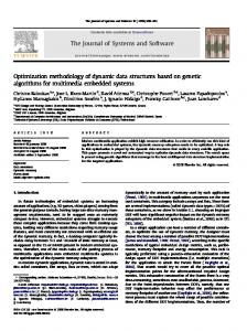
produced renewable energy while (ii) during time interval [t2, t3], a surplus of renewable energy production is predicted which cannot be used to operate the DC since the predicted energy consumption levels are small for that time interval.

The constraints are used in the decision process to define and validate specific energy charging and discharging actions against the energy storage device characteristics. They are defined in a similar manner as for the TES (see relations 1-7). The only constraint that changes in the energy storage case is expressed by the relation 4 that now expresses the following constraint “The action of discharging the energy storage device cannot decrease the amount of stored energy below the defined Depth of Discharge limit”:

To optimize the above presented situation, our methodology will first determine the amount of flexible energy available in the DC during time interval [t1, t2] using the flexibility mechanisms already defined. Then it will optimize the DC operation so that the hashed amount of energy (the demanded extra energy) in the interval [t1, t2] will be delayed through flexible energy shifting mechanisms to be consumed in the time interval [t2, t3].

𝐷𝑜𝐷 ∗ 𝑀𝐴𝑋𝐸𝑆𝐷 ≤ 𝐸𝑆𝐷𝑙𝑒𝑣𝑒𝑙 (𝑡) ≤ 𝑀𝐴𝑋𝐸𝑆𝐷

(14)

The flexibility mechanism defined for an energy storage device works as follows: (i) the amount of energy discharged from the device at timeslot t is compensated with an equal amount of energy saved by not using renewable energy produced locally or taken from the grid and (ii) the amount of energy charged in the device at moment t is compensated with an equal amount of renewable energy consumed by the DC. D. Diesel Generators Flexibility In addition to the power supplied by the grid or by local renewable energy sources, DCs use diesel generators that can produce enough energy to cover the electricity demand in case of an emergency. Due to the time inertia of diesel generator operation, until their full operational status, the DC is powered by the UPS units. The diesel generators need periodic maintenance and during this process they may also produce a certain amount of energy which can be used. We denote the maximum power supplied by the generators with 𝑀𝐴𝑋𝐺𝐸𝑁 and we consider that during maintenance they are running at a certain percentage of the maximum capacity.

Fig. 1. Renewable energy consumption and production in a non-optimal DC operation situation

Figure 2 presents a possible situation of the optimized DC operation. It can be seen that the energy demand is shifted and now the DC energy consumption curve (dashed line) follows the renewable energy production curve (solid line). In other words, we have planned a DC energy consumption peak to match the predicted renewable energy production peak.

We will exploit this potential flexibility by planning the periodic maintenance in moments of renewable energy production deficits. IV. RENEWABLE ENERGY USAGE OPTIMIZATION METHODOLOGY We have defined an optimization methodology which exploits the energy consumption flexibility at the DC level to shift the energy demand so that the renewable energy produced locally is used as much as possible in the DC operation. In other words, the methodology aims to plan the DC operation by exploiting various flexibility mechanisms presented in section III so that the DC energy consumption curve will match or follow the renewable energy production curve. For example let us consider the DC operation situation presented in Figure 1. The solid line curve represents the predicted amount of renewable energy over a time window, while the dashed line curve represents the predicted amount of DC energy consumption over the same time window. This situation is inefficient from two reasons: (i) during time interval [t1, t2], high levels of energy consumption are predicted which cannot be covered by using the estimated amounts of locally

Fig. 2. Renewable energy consumption and production after optimization

The algorithm from Figure 3 presents the pseudo-code description of the optimization methodology. The algorithm has as inputs the forecast renewable energy production and energy consumption curves over a fixed time window. The output will be flexible energy consumption adjustments over the time window, so that in the end the actual DC energy consumption curve will follow the renewable energy production curve. The algorithm starts by evaluating in parallel the amount of flexible energy available in the DC at each moment of the analyzed timeframe. We use the flexibility mechanisms and valid optimization actions for the DC components that provide flexibility and are defined in Section III (lines 5-8). At each step the flexible energy is shifted in different combinations and for

each combination the estimated DC energy consumption and production values are calculated (lines 11-12).

as the degree of prediction accuracy by using two levels of granularity: intra-day (few hours ahead) and near real-time (few minutes ahead). Due to the inherent inaccuracy of the predicted data, errors may appear and as such corrective actions must be considered for the next few hours or for the next few minutes. It should be noted that the closer we get to the real time, the cost of implementing the corrective actions becomes higher.

The DC energy consumption is estimated as the sum of the energy consumption of IT components that execute the DC workload, the energy consumed by the cooling system and the energy used to charge the DC electrical storage devices: 𝐸𝐷𝐶𝑐𝑜𝑛𝑠𝑢𝑚𝑝𝑡𝑖𝑜𝑛 (𝑡) = 𝐸𝑤𝑜𝑟𝑘𝑙𝑜𝑎𝑑 (𝑡) + 𝐸𝑐𝑜𝑜𝑙𝑖𝑛𝑔 (𝑡) + 𝑅_𝐸𝑆𝐷𝑢𝑠𝑎𝑔𝑒 (𝑡)

(15)



Intra-day DC operation planning refines, adjusts and improves the plan of actions determined in the previous day by using a finer prediction on a smaller time window, in this case few hours ahead. It is capable of modifying the parameters and the optimization actions already scheduled by the day ahead DC operation planning algorithm to further exploit the DC energy flexibility mechanism by using better predicted data.



Near real-time DC operation planning allows further correcting the scheduled energy consumption optimization actions to the real-time execution conditions with a reaction time of few minutes.

Fig. 4. Renewable Energy Usage Optimization Methodology Loops

Fig. 3. Algorithm used to maximize the usage of locally produced renewable energy for DC operation

The DC energy production is estimated as a sum of the amounts of energy produced from renewable sources and the energy discharged from energy storage devices and used to power up the DC. 𝐸𝐷𝐶𝑝𝑟𝑜𝑑𝑢𝑐𝑡𝑖𝑜𝑛 (𝑡) = 𝐸𝑟𝑒𝑛𝑒𝑤𝑎𝑏𝑙𝑒 (𝑡) + 𝐷_𝐸𝑆𝐷𝑢𝑠𝑎𝑔𝑒 (𝑡)

(16)

Finally, the algorithm determines the optimal flexible energy amount generated by combining the available flexible energies produced by the appropriate DC elements such that the difference between the estimated energy consumption and production curves is minimized (line 20). The methodology has three different loops with different time granularities (see Figure 4): 

Day-ahead operation planning decides on the energy flexibility optimization actions for the next operational day. During the next operational day, the execution of the decided optimization action plan is tracked as well

The process of forecasting the DC energy production and consumption levels is out of the scope of this paper. Briefly, the forecast values are determined using the time series prediction technique on historical data defined by us in [12]. The amount of energy consumed and produced by the DC is being continuously monitored; the actual values and their timestamps are being collected and stored at regular sampling periods are generating two different time series. The time series are then analyzed for identifying frequent energy consumption or generation patterns. A sliding window based method is employed to identify whether the actual energy consumption or generation features match an already determined frequent energy consumption pattern. For accurately predicting DC’s renewable energy production, weather data is considered. The energy production patterns are associated with the weather conditions from the timeframe when the observation was made. V. USE CASE EVALUATION To evaluate the proposed technique and mechanism we have developed a simulation environment in which we have simulated the operation of a DC having installed the components from Table 1. The DC renewable energy is produced by means of wind turbines.

TABLE I.

MODELED DC COMPONENTS CHARACTERISTICS

Component Electrical cooling

IT Server

Battery

TES

Wind Turbines

Diesel Generator

Property Cooling capacity Minimum cooling load COP Coefficient Maximum Cooling Load P_IDLE P_MAX Memory Processor Hard Drive Charge Loss rate Discharge Loss rate Energy Loss rate Max Discharge rate Maximum Capacity Max Charge rate Energy Loss rate Charge Loss rate Discharge Loss rate Max Discharge rate Maximum Capacity Max Charge rate Max Capacity Air Density Blade length Power Coefficient Max Capacity

Value 4000 kW 200 kW 3.5 2000 kW 190 W 325 W 8 GB, 266MHz 2.4 GHz 2 Cores 1Tb, 7200 RPM 1.2 0.8 0.995 1000 kW 1000 kW 1000 kW 0.999 1.1 0.99 1000 kW 3000 kW 1000 kW 1000 kW 1.23 40 m 0.4 3000 kW

The DC operation simulation data is generated at fixed time intervals using the data sources presented in Table 2. TABLE II.

Data Generated Workload Energy Consumption

Weather Data

Cooling Energy Consumption

SIMULATION DATA SOURCES

Data Sources

Description

IT power consumption logs of real DC [13]

Real-time workload as IT power consumption sampled every 5 minutes and normalized considering the maximum amount of power consumption of modeled DC. Wind speed

Online weather forecast services [14] Percentage of workload energy consumption [15]

We have defined an evaluation scenario in which the forecasted renewable energy production exhibits spikes which are higher than the DC energy consumption. We have considered a prediction confidence interval for the forecasted energy budget of +10%. In this scenario, optimization actions are taken for exploiting the energy flexibility at the DC level aiming at shifting the flexible energy load to match the renewable energy production curve. Figure 5 presents the forecasted DC energy consumption values for the next 24 hours split into cooling energy consumption, delay tolerable workload energy consumption and real time workload energy consumption. Also renewable energy production values are represented in the figure.

Fig. 5. Renewable energy consumption and production after optimization

Figure 5 forecasted energy budget represents a non-optimal DC operation situation: (i) during the first operational hour (hour 0) the DC energy consumption is predicted to be higher than the energy production, (ii) between the hours 2 and 10 there is predicted a spike of renewable energy production which cannot be consumed by the DC given its current operation plan, (iii) between the hours 11 and 18 there will be a burst of energy consumption and (iv) between the hours 18 and 23 there is predicted a spike of renewable energy production which cannot be consumed by the DC. The defined optimization methodology will correct this situation and decide an optimization action plan (see Figure 6) that will shift the energy consumption demand from the first operational hour to the operational 2 and 3 when the renewable energy spike is predicted.

Considering Cooling COP value 3.5

The optimization action plans execution has been simulated by implementing simple stubs for each type of DC components. The stubs role is to determine the energy impact of action execution by considering the technical characteristics of the affected DC component.

Fig. 6. Optimization action plan and associated energy impact

During the renewable energy spike the energy surplus is saved by charging the TES. This will allow decreasing the DC high energy consumption from hours 11 to 18 by discharging the TES and using at lower intensity the electrical cooling. Also

the delay tolerable workload from hours 11 to 18 is executed as much as possible to the time interval 18 to 23. Also, by looking at Figure 6 one can notice that by executing the “Optimization Action Plan 1” decided the DC energy consumption curve will manage to follow the renewable energy production curve.

renewable energy). At the same time with optimization the energy demand is shitted in such a manner so that the renewable energy surplus is all consumed.

The intra-day and near real-time optimization process will follow the above plan execution and decides if needed (i.e. missprediction of renewable energy spikes) new actions to correct and improve the DC operation using smaller time scale and more accurate predictions. Figure 7 presents the improved energy budget resulted after executing corrective actions decided by the intra-day optimization for the first 4 operational hours.

Fig. 9. Near real-time DC energy consumption and production with and without optimization between simulation hours 2 and 4

Fig. 7. Optimization action plan an associated energy impact

Figure 8 presents the evolution of DC energy consumption in near real-time fashion with our optimization technique activated and without for the first 2 simulation hours (between simulation hours 0 and 2). One can notice that without the optimization activated the energy consumption demand is higher than the renewable energy production and brown energy is consumed from the grid to compensate (see “Energy Sources Without Optimization” – blue color represents the energy from the grid). On contrary when optimization methodology is used the energy demand in this two hours is shifted in such a way that only the renewable energy is used.

After running the simulation on the presented scenario for 24 hours the amount of renewable energy used for DC operation in the optimization case has increased of 12% percent. This translates in an increase of renewable energy amount used of 5400 kWh for 24 hours. The total power consumption of the DC simulated is about 45000 kWh. To assess the positive environmental impact of our methodology we have used the UK Department for Environment, Food & Rural Affairs study that states that by producing 1 kWh of electrical energy, results in about 0.527 kg of CO2 which is released in the atmosphere [17]. Considering our optimization methodology running for 24 hours and the increased values of renewable energy used in detriment of the brown energy we have estimated the total CO2 emissions saving of about 3056 kg of CO2. VI. CONCLUSIONS In this paper, we have presented a methodology for shifting the DC energy consumption from an original baseline pattern to match the renewable energy supply levels. The methodology uses different flexibility mechanism for components such as electrical cooling system, IT workload, energy storage and diesel generators. As a result an increased amount of locally produced renewable energy is used in DC operation. The in-lab results obtained using simulations are promising showing that our methodology manages to increase to usage of renewable energy with about 12%.

Fig. 8. Near real-time DC energy consumption and production with and without optimization between simulation hours 0 and 2

As future work we plan to use the defined methodology in the pilot DCs of the EU FP7 GEYSER project [16]. Also we plan to improve our methodology to take into account (beside the renewable energy levels) new criteria such as the energy price, the smart grid context or the demand for ancillary services. ACKNOWLEDGMENT

For the next operational hours (between simulation hours 2 and 4) without optimization the DC will lose the surplus of renewable energy produced (see Figure 9 – “Energy Sources Without Optimization” – red color which represents the unused

This work has been partially supported by the GEYSER project [16] and has been partly funded by the European Commission ICT activity of the 7th Framework Program (contract number 609211). This work expresses the opinions of

the authors and not necessarily those of the European Commission. The European Commission is not liable for any use that may be made of the information contained in this work. REFERENCES [1]

[2]

[3]

[4]

[5]

[6]

[7]

IBM Report, “The green data center: cutting energy costs for a powerful competitive advantage”, Online, 2008, https://www304.ibm.com/businesscenter/cpe/download0/153971/The_Green_Data_ Center.pdf I. Goiri, W. Katsak, K. Le, T. D. Nguyen, and R. Bianchini, “Parasol and GreenSwitch: Managing Datacenters Powered by Renewable Energy”, Proceedings of the International Conference on Architectural Support for Programming Languages and Operating Systems (ASPLOS), 2013. C. Chen, B. He, X. Tang, C. Chen, Y. Liu, “Green Databases Through Integration of Renewable Energy”, Conference on Innovative Data Systems Research (CIDR), 2013. Z. Liu, Y. Chen, C. Bash, A. Wierman, D. Gmach, Z. Wang, M. Marwah, and C. Hyser, “Renewable and cooling aware workload management for sustainable data centers”, SIGMETRICS Perform. Eval. Rev. 40, 1, 175186, 2012. R. Carroll, S. Balasubramaniam, D. Botvich, W. Donnelly, “Application of Genetic Algorithm to Maximise Clean Energy Usage for Data Centres”, Bio-Inspired Models of Network, Information, and Computing Systems, 2012. C. Li, A. Qouneh, and T. Li, “iSwitch: coordinating and optimizing renewable energy powered server clusters”, In Proceedings of the 39th Annual International Symposium on Computer Architecture, 2012. Y. Zhang, Y. Wang, and X. Wang, “GreenWare: greening cloud-scale data centers to maximize the use of renewable energy”, In Proceedings of

[8]

[9]

[10] [11] [12]

[13]

[14] [15]

[16] [17]

the 12th ACM/IFIP/USENIX international conference on Middleware, 2011. R. L. Sawyer, “Calculating Total Power Requirements for Data Centers”, Whitepaper, Online at http://www.apcmedia.com/salestools/vavr5tdtef/vavr-5tdtef_r1_en.pdf?sdirect=true Y. Zhang, Y. Wang, and X. Wang, “TEStore: Exploiting Thermal and Energy Storage to Cut the Electricity Bill for Datacenter Cooling”, 8th international conference and workshop on systems virtualization management, 2012. Q. Tang, “Sensor-Based Fast Thermal Evaluation Model for Energy Efficient High-Performance Datacenters”, Intel Corporation, 2006. W. Zheng, K. Ma, and X. Wang, “Exploiting Thermal Energy Storage to Reduce Data Center Capital and Operating Expenses”, HPCA, 2014. T. Cioara, I. Anghel, I. Salomie, G. Copil, D. Moldovan, M. Grindean, “Time Series based Dynamic Frequency Scaling Solution for Optimizing the CPU Energy Consumption”, IEEE 7th International Conference on Intelligent Computer Communication and Processing Special Session: Green Computing, pp. 477 - 483, ISBN: 978-1-4577-1479-5, 2011. C. Wang, B. Urgaonkar, Q. Wang, G. Kesidis, and A. Sivasubramaniam, “Data Center Power Cost Optimization via Workload Modulation,” UCC, 2013. Forecast For Developer API, Online at http://forecast.io/ J. Moore, J. Chase, P. Ranganathan, “Making scheduling cool: temperature-aware workload placement in data centers”, Proceedings of the annual conference on USENIX annual technical conference, 2005. GEYSER FP7 project, http://www.geyser-project.eu/ UK Department for Environment, Food & Rural Affairs (DEFRA), Act on CO2 Calculator: Public Trial Version Data, Methodology and Assumptions Paper, June 2007,