Data Collection Capacity of Random-Deployed Wireless ... - CiteSeerX

Data Collection Capacity of Random-Deployed Wireless Sensor Networks Siyuan Chen∗ ∗ Department

Yu Wang∗

Xiang-Yang Li†

Xinghua Shi‡

of Computer Science, University of North Carolina at Charlotte, Charlotte, North Carolina, USA of Computer Science, Illinois Institute of Technology, Chicago, Illinois, USA ‡ Department of Computer Science, University of Chicago, Chicago, Illinois, USA

† Department

Abstract— Data collection is one of the most important functions provided by wireless sensor networks. In this paper, we study the theoretical limitations of data collection and data aggregation in terms of delay and capacity for a wireless sensor network where n sensors are randomly deployed. We consider two different communication scenarios (with or without aggregation) under physical interference model. For each scenario, we first propose a new collection method and analyze its performance in terms of delay and capacity, then theoretically prove that our method can achieve the optimal order. Particularly, the capacity of data collection is in order of Θ(W ) where W is the fixed data-rate on individual links. If each sensor can aggregate its receiving packets into a single packet to send, the capacity of data collection increases to Θ( logn n W ).

I. I NTRODUCTION For wireless sensor networks, often the ultimate goal is to collect the sensing data from all sensors to a sink node and then perform further analysis at the sink node. Thus, data collection is one of the most common services used in sensor network applications. In this paper, we study some fundamental capacity problems arising from different types of data collection scenarios in wireless sensor networks. For each problem, we will derive the asymptotic upper bound of transport capacity and present efficient algorithms to achieve such upper bound with certain constant factor. We consider a dense sensor network where n sensors are randomly deployed in a finite geographical region. Each sensor measures independent field values at regular time intervals and send these values to the sink. The union of all sensing values from n sensors at particular time is called snapshot. The task of data collection is to deliver these snapshots to the sinks. Due to spatial separation, several sensors can successfully transmit at the same time if these transmissions do not cause any destructive wireless interferences. We assume that a successful transmission over a link has a fixed data-rate W bit/second. The work of Y. Wang is supported in part by the US National Science Foundation (NSF) under Grant No. CNS-0721666 and No. CNS-0915331. The work of X.-Y. Li is partially supported by the US NSF under Grant No. CNS-0832120, the National Natural Science Foundation of China under Grant No. 60828003, No.60773042 and No.60803126, the Natural Science Foundation of Zhejiang Province under Grant No. Z1080979, the National Basic Research Program of China (973 Program) under Grant No. 2006CB30300, the National High Technology Research and Development Program of China (863 Program) under Grant No. 2007AA01Z180, the Hong Kong RGC under Grant HKUST 6169/07, HKBU 2104/06E, and CERG under Grant PolyU5232/07E. X.-Y. Li is also with Institute of Computer Application Technology, Hangzhou Dianzi University, Hangzhou, China.

The performance of data collection in sensor networks can be characterized by the rate at which sensing data can be collected and transmitted to the sink node. In particular, the theoretical measures that capture the possibilities and limitations of collection processing are delay and capacity for the many-to-one data collection. The delay of data collection is the time to transmit one single snapshot to the sink from the snapshot generated at sensors. Considering the size of data in the snapshot, we can define delay rate as the ratio between the data size and the delay. When multiple snapshots from sensors are generated continuously, data transport can be pipelined in the sense that further snapshot may begin to transport before the sink receiving the prior snapshot. The maximum data rate at the sink to continuously receive the snapshot data from sensors is defined as the capacity of data collection. Both delay rate and capacity reflect that how fast the sink can collect sensing data from all sensors. It is critical to understand the limitations of many-to-one information flows and devise efficient data collection algorithms to maximize performance of wireless sensor networks. In this paper, we are particularly interested in how delay rate and capacity of data collection vary as the number of sensors n increases. Gupta and Kumar initiated the research on capacity of random wireless networks in the seminal paper [1]. A number of following papers studied capacity under different communication scenarios [2]–[4]. Recently, capacity limits of data collection in random wireless sensor networks have been studied in the literature [5]–[11]. In [5], [6], Duarte-Melo et al. first studied the many-to-one transport capacity in dense and random sensor networks. But they only considered the simplest case with a single sink under protocol interference model. Chen et al. [7] studied capacity of data collection with multiple sinks in random networks under protocol interference model. Liu et al. [8] recently studied the capacity of a general someto-some communication paradigm under protocol interference model in random networks where there are multiple randomly selected sources and destinations. All these works are based on protocol interference model. El Gamal [9] studied the capacity of data collection subject to a total average transmitting power constraint where a node can receive data from multiple source nodes at a time. Barton and Rong [10], [11] then investigated data collection capacity under more complex physical layer models (non-cooperative SINR model and cooperative time reversal communication model) where the data rate of indi-

vidual link is not fixed as a constant W but depended on the level of interference. In this paper, we study capacity of data collection under physical interference model for random sensor networks with a single sink. The major contributions of this paper are as follows. (1) For sensor networks without data aggregation, we propose a new data collection method whose delay rate and capacity under physical interference model are both Θ(W ) which match the theoretical upper bounds in order. (2) By using data aggregation [12], [13] where sensors can cooperate to aggregate information towards the sink, the communication overhead is reduced and the capacity is increased. We theoretically prove that√ the delay rate and the capacity of data aggregation are Θ( n log nW ) and Θ( logn n W ) respectively. For both cases, our proposed collection/aggregation methods achieve the optimal orders (i.e., within a constant factor of upper bounds). II. P RELIMINARIES A. Network Model We consider a sensor network which includes n wireless sensor nodes V = {v1 , v1 , · · · , vn } and a single sink node s. Here, we assume that both sensor nodes and the sink node are uniformly deployed in a square region with side-length √ a = n, by use of Poisson distribution with density 1. At regular time intervals, each sensor node measures the field value at its position and transmits the value to the sink node. We adopt a fixed data-rate channel model where each wireless node can transmit at W bits/second over a common wireless channel. Under such channel model, we assume that every node has a fixed transmission power. Then a fixed transmission range r can be defined such that a node vi can successfully receive the signal sent by node vj only if the distance between them is less or equal to r. We also assume that all packets have unit size b bits. The time is slotted into time slots with t = b/W seconds. Thus, only one packet can be transmitted in a time slot between two neighboring nodes. As in the literature, we consider the interference modeled by physical interference model in our analysis. In physical interference model, node vj can correctly receive the signal from the sender vi if and only if, given a constant η > 0, the SINR Pi · l(||vi − vj ||) P ≥ η. B · N0 + k∈I Pk · l(||vk − vj ||) Here ||vi − vj || is the Euclidean distance between vi and vj , l(x) is the transmission loss during a path of length x, B is the channel bandwidth, N0 > 0 is the background Gaussian noise, I is the set of actively transmitting nodes when node vi is transmitting, and Pk is node vk ’s transmission power. In this paper, we consider the attenuation function l(x) = min{1, x−β } where β > 2 is the path loss exponent. Hereafter, we assume that each sensor uses the same transmission power P , and all N0 , β and η are fixed constants. Notice that values of P , N0 , η, and transmission range r should satisfy P ·r −β ≥ η. Thus, r ≤ ( B·N )1/β . that PBN 0 0 ·η

sink node s in cell (p, q) (0, m)

1111111111111 0000000000000 0000000000000 1111111111111 0000000000000 1111111111111 0000000000000 1111111111111 0000000000000 1111111111111 0000000000000 1111111111111 0000000000000 1111111111111 0000000000000 1111111111111 0000000000000 1111111111111 0000000000000 1111111111111 0000000000000 1111111111111 0000000000000 1111111111111 d 0000000000000 1111111111111 (0, 0)

(m, m)

1/2

a=n

(m, 0)

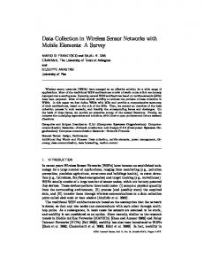
Fig. 1. Grid partition of the sensor network: a2 cells with cell size of d × d.

B. Capacity and Delay We now formally define delay and capacity of data collection. Recall that each sensor at regular time intervals generates a field value with b bits and wants to transport it to the sink. We call the union of all values from all n sensors at particular sampling time a snapshot of the sensing data. The goal of data collection is to collect these snapshots from all sensors as quick as possible. Definition 1: The delay of data collection ∆ is the time transpired between the time a snapshot is taken by the sensors and the time the sink has all data of this snapshot. Definition 2: The delay rate of data collection Γ is the ratio between the data size of one snapshot n · b and the delay ∆. On the other hand, the data transport can be pipelined in the sense that further snapshots may begin to transport before the sink receiving the prior snapshots. Therefore, we need to define a new data rate of data collection under pipelining. Definition 3: The usage rate of data collection U is the number of time slots needed at the sink between completely receiving one snapshot and completely receiving next snapshot. Thus, the time used by the sink to successfully receive a snapshot is T = U × t. Due to pipelining, T ≤ ∆. Clearly, small usage rate and T are desired. Definition 4: The capacity of data collection C is the ratio between the size of data in one snapshot and the time to receive such a snap shot (i.e., nb T ) at the sink. Thus, the capacity C is the maximum data rate at the sink to continuously receive the snapshot data from sensors. Clearly, C is at least as large as the delay rate Γ, and usually substantially larger. In this paper, we analyze both delay rate and capacity for data collection in random sensor networks. III. DATA C OLLECTION WITHOUT AGGREGATION In this section, we consider data collection without aggregation where each data packet generated from a sensor needs to individually reach the sink s. We first construct a data collection scheme whose delay rate is Ω(W ), and then prove that it is order-optimal. Our data collection scheme is based on the following grid partition method.

A. Our Partition Method (a/2L,a/2L)

We first introduce a grid partition method which is essential for our data collection methods and their theoretical analysis. As shown in Fig. 1, the network (e.g., the a × a square) is divided into m2 micro cells of the size d × d. Here m = a/d. We assign each cell a coordinate (i, j), where i and j are between 1 and m, to indicate its position at jth row and ith column. The following lemma gives a guidance of the cell size. √ √ Lemma 1: [14] Given n random nodes in a n × n square, dividing the square into micro cells of the size √ √ 3 log n × 3 log n, every micro cell is occupied with probability at least 1 − n12 . q √ n Therefore, if we set d = 3 log n (i.e., m = 3 log n ), every micro cell has at least one node with high probability (the probability converges to one as n −→ ∞). We then derive the upper bound of the number of nodes inside a single cell. √ √ Lemma 2: Given n random nodes in a n × √n square, dividing the square into micro cells of the size 3 log n × √ 3 log n, the maximum number of nodes in any cell is n O(log n) with probability at least 1 − 3 log n . Proof: The proof is straightforward from results of the balls into bins problem [15] and thus ignored here. In order to make the whole network connected, √ the transmission range r need to be equal or larger than 5d so that any two nodes from two neighboring cells are √ inside each √ other’s transmission range. Hereafter, we set r = 5d = 15 log n.

(i,j)

(1,0)

(0,1)

L

Grid partition of interference blocks with size of L × L.

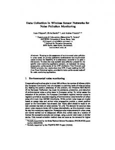
Fig. 2.

Based on physical interference model, its SINR is B · N0 +

P · l(r)

P

all blocks (i,j) except (0,0)

P · l(di,j )

.

Here, di,j is the distance from the sender in block (i, j) to the receiverpin block (0, 0). By a simple geometric calculation, √ di,j = (iL − d)2 + (jL − 2d)2 . Remember r = 15 log n thus both r and di,j are larger than 1. Therefore, we need to derive L such that B · N0 +

P

P · r−β ≥ η. 2 2 −β/2 (i,j)/(0,0) P · ((iL − d) + (jL − 2d) )

In other words, we need

B. Our Data Collection Scheme As shown in Fig. 1, we can consider data collection of nodes from four different directions (i.e., quadrants) to the sink s located in cell (p, q). For the purpose of analysis, we only concentrate on the direction which has the largest number of sensors, e.g., the shaded rectangle in Fig. 1, since the sink can perform collection on each direction in turn and it only adds a constant 4 in the analysis. Furthermore, here we only consider the worst case where p = q = m, that is, the sink is in the upper right corner of the field. For our collection scheme, we first divide the field into big blocks with size L × L as shown in Fig. 2. We call these blocks interference blocks and L interference distance. Thus, 2 the number of interference blocks is ⌈ La 2 ⌉. We label each block with (i, j) where i and j are the indexes of the block as in Fig. 2. In our collection scheme, we schedule data transmission in parallel at all blocks but make sure that there is only one sensor in each interference block transferring at any time. To avoid interference from senders in other interference blocks, we need interference distance L larger than certain value. Next, we derive the lower bound of interference distance such that all simultaneous transmissions as shown in Fig. 2 can be successfully received. Here, we consider the SINR at the receiver in interference block (0, 0) (which is in the center of the field) since it has the minimum SINR among all receivers.

(0,0)

d

dij

X

((iL − d)2 + (jL − 2d)2 )−β/2 ≤

(i,j)/(0,0)

BN0 r−β − . η P

Notice that: X

((iL − d)2 + (jL − 2d)2 )−β/2

X

((iL − 2id)2 + (jL − 2jd)2 )−β/2

(i,j)/(0,0)

≤ =

(i,j)/(0,0)

(L − 2d)−β

X

(i2 + j 2 )−β/2 .

(i,j)/(0,0)

Instead of considering interference from all blocks (i, j) around (0, 0), we relax it to 4 times the interference from blocks in the right up direction. X ((iL − d)2 + (jL − 2d)2 )−β/2 (i,j)/(0,0)

≤ (L − 2d)−β

X

(i,j)/(0,0)

X

−β

≤ 4(L − 2d) =

−β

4(L − 2d)

(i2 + j 2 )−β/2 (i2 + j 2 )−β/2

(i≥0,j≥0)/(0,0)

(

X

(i≥1,j≥1)

(i2 + j 2 )−β/2 + 2

X

(i≥1,j=0)

i−β ).

(m,m)

(m,m)

L

(0, 0)

(m,m)

L

(0, 0)

L

(a) Phase I, 1st time slot Fig. 3.

L

(0, 0)

L

(b) Phase I, 2nd time slot

(m,m)

L

L

(c) Phase II, 1st time slot

(0, 0)

L

(d) Phase II, 2nd time slot

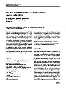
Our collection method: [Phase I] each node send its data to its upper cell; [Phase II] each node in the top row send its data to its right cell.

1 β/2 Notice that for i > 1, j > 1 and β > 2, ( i2 +j ≤ 2) 1 1 1 1 1 1 β/2 ≤ 2β ( iβ + j β ). Then we have ( 4 ( i2 + j 2 )) X ((iL − d)2 + (jL − 2d)2 )−β/2

In each phase, the data transmissions in all interference blocks are performed in parallel. C. Analysis of Delay Rate

Now we analysis the delay rate of our data collection scheme above. We define the time needed for the two phases 4(L − 2d) ( (i + j ) +2 i ) as T1 and T2 , respectively. (i≥1,j≥1) (i≥1,j=0) By Lemma 2, the number of nodes in each cell is at most X X 1 1 1 −β O(log n). Every node needs one time-slot t to send one packet ( + ) + 2 i ) 4(L − 2d)−β ( 2β iβ jβ to its neighbor in the next cell. To avoid interference, every (i≥1,j=0) (i≥1,j≥1) X X 1 X 1 interference block can only have one node send a packet to its 1 1 4(L − 2d)−β ( β + β +2 i−β ) upper neighbor in every time slot t during Phase I. In Fig. 3, β β 2 i 2 j i≥1 i≥1 j≥1 bold lines show the interference blocks. Remember that Ld is a X 1 constant α, thus the number of cells in the interference block i−β 4(L − 2d)−β ( β−1 + 2) 2 is ( Ld )2 = α2 . And the packet in the lowest row (i.e. cell i≥1 (0, k)) has to walk m cells to reach nodes in the highest cell X 1 i−2 4(L − 2d)−β ( β−1 + 2) in the rectangle. Hence, 2 (i,j)/(0,0)

≤ ≤ = = ≤ ≤

−β

X

2

2 −β/2

X

−β

i≥1

∞ X 2π π 1 i−2 = ). (L − 2d)−β ( β−1 + 2) (since 3 2 6 i=1

T1

1 −β 0 + 2) ≤ r η − BN Therefore, if 2π ( 2β−1 3 (L − 2d) P , we can sure that the SINR at the receiver in the center is at least η. This can be satisfied by setting −β

L≥(

r−β BN0 − β1 3 · 2(β−2) + 2d. · ( − )) π(1 + 2β ) η P

P Remember r ≤ ( B·N )1/β , this makes sure we can find 0 ·η (β−2)

3·2 r − such suitable L. We can further select L = ( π(1+2 β) · ( η √ 1 − BN0 β + 2d. Since r = 5d, P )) √ L 3 · 2(β−2) ( 5d)−β BN0 − β1 +2 = ( ·( − )) β −β d π(1 + 2 ) ηd P d−β 3 · 2(β−2) 5−β/2 BN0 dβ − β1 = ( + 2. · ( − )) π(1 + 2β ) η P −β

When n → ∞, this ratio goes to a constant, denoted by α. After having interference blocks, we can now present our collection algorithm which is quite simple and straightforward. It has two phases. In Phase I, every sensor sends its data up to the highest cell in its column (in the ath row) as shown in Fig. 3(a) and Fig. 3(b), and in Phase II, all data is sent via cells in the ath row to the sink as shown in Fig. 3(c) and Fig. 3(d).

L ≤ ( )2 × t × O(log n) × m d r

≤ O(t log n)m = O(t log n)

p n = O(t n log n). 3 log n

In the beginning of Phase II, all data are already at cells of the top row. The sink s lies on the same row with these cells. We now estimate T2 needed for sending all data to s. Each cell in the top row has at most mO(log n) nodes’ data and the number of cells in each interference block is Ld . Similarly, we can get L × t × mO(log n) × m ≤ m2 O(t log n) = O(nt). d Therefore, the total time needed to collect b-bits information from every sensor in the field to the sink is T1 + T2 = O(nt). Thus, the total delay ∆col for the sink to receive a complete snapshot is at most O(nt). Consequently, the total delay rate of this collection scheme is nb nb Γcol = = Ω( ) = Ω(W ). ∆col nt T2 ≤

It has been proved that the upper bound of delay rate or capacity of data collection is W [5], [6]. It is obvious that the sink cannot receive at rate faster than W since W is the fixed transmission rate of individual link. Therefore, the delay rate of our collection scheme achieves the order of the upper

(m,m)

(m,m)

bound, and the delay rate of data collection is Θ(W ). Notice that for each individual sensor the lowest achievable delay rate of our method is Θ(W/n) which also meets the upper bound. D. Capacity of Data Collection Next, we consider the situation with pipelining. It is clear the upper bound of capacity is still W . Since our above scheme already reaches the upper bound, the pipelining operation can only improve the capacity within a constant factor. With pipelining, in Phase I, the sensor can begin to transfer the data to its up-cell from next snapshot after sensors in its interference block finish their transmission of previous snapshot. Whenever the cells in the top row receive m · b data (every cell in the top row receives a data from its lower cell), Phase II can begin at the top row. We consider the improvements of pipelining on both phases. With the pipelining, the time T1′ for the highest cell to receive a new set of m · b data in Phase I is L T1′ ≤ ( )2 × t × O(log n) = O(t log n). d And the time in Phase II is

T2′

for the sink to receive a new set of a · b data

T2′ ≤

L × t × m = O(t d

r

n ). log n

Therefore, q the total time for sink to receive m · b data is T1′ + ′ T2 = O(t logn n ). Thus, the capacity of our method with pipelining is still Ccol =

m·b = Ω(W ). T1′ + T2′

This also meets the upper bound W in order. In summary, we have the following theorem: Theorem 1: Under physical interference model, the delay rate Γ and the capacity C of data collection in random sensor networks with a single sink are both Θ(W ). IV. DATA C OLLECTION WITH AGGREGATION In this section, we investigate a different data collection scenario where each sensor can aggregate its received data (multiple packets) into a single packet. For example, if the sink just wants to know the maximal temperature in the deployed field, then each sensor can send out the maximal sensing value towards the sink instead of all values which it receives from other sensors. Here, we study both delay rate and capacity of data aggregation with a single sink. The definitions of delay rate and capacity are similar to those of data collection in Section II. Notice that when the sink receives the maximal value (just b bits) of a snapshot of the field (n sensors), we still count the size of all values from that snapshot as the size nb of the received data. Thus, delay rate is nb ∆ and capacity is T . There is not much work on capacity of data aggregation in wireless sensor networks, except for [12] and [13]. Giridhar and Kumar [12] investigated a more general aggregation problem in random sensor network where a symmetric function of

0 L 11 1 0 1 1111 0000 0 00 1 0 1 0000 1111 00 11

(0, 0)

(0, 0)

(a) Phase II

(b) Phase III

Fig. 4. Our aggregation method: [Phase II] each selected node aggregates data to its upper cell; [Phase III] each selected node in the top row aggregates data to its right cell.

the sensor measurements is used for data aggregation. Moscibroda [13] then further studied the aggregation capacity for arbitrarily deployed networks under both protocol interference model and physical interference model. A. Analysis of Delay Rate We again assume that the sink s is located in cell (m, m). Our aggregation scheme has three phases and uses the same partition method in Section III. First, each micro cell chooses a sensor which collects data from all the other sensors in the same micro cell and aggregates into one packet. Based on Lemma 2, each micro cell has at most O(log n) nodes. Assume that T1′′ is the time needed to collect data inside each cell. Because of the interference distance R, T1′′ is at most ( Ld )2 · O(log n) · t. Second, every selected node waits for all data in the same snapshot from cells, which are below its own cell and within the same column, and then aggregates them with its value into a single packet and sends it to its upper cell. See Fig. 4(a). At the end of this phase, all value has been aggregated at the top row where the sink sits. The time needed for this q phase T2′′ is bounded from above by m × t × ( Ld ) = Θ( logn n t), since every Ld columns only one node can transmit due to interference, as shown in Fig. 4(a). Third, as shown in Fig. 4(b), the information is aggregated ′′ via cells one by one q in the top row. The time needed T3 is at n most m × t = Θ( log n t). Therefore, the total delay ∆agg ≤ T1′′ + T2′′ + T3′′ = q n O( log n t). The delay rate is Γagg =

p nb = Ω( n log n · W ). ∆agg

Next, we prove that this delay rate is order-optimal. Notice that for one snapshot the data aggregation is completed when the sink has the aggregated value of all data in the snapshot. Let Tcomplete denote the time that all data of one snapshot are aggregated in the sink and Tf arthest be the time needed for the value of the farthest node reaching the sink. Since to compute the aggregated value, all values from the snapshot are needed, Tf arthest ≤ Tcomplete . Based on the network model,

the farthest node from the sink locates on one corner of the field. We denote the distance between the farthest node and the sink √ as R. It is easy to show that the minimum value of R is √ 22a (when the sink is in the center of the field), i.e. R ≥ 22n . The data in the farthest node needs at least Rr time slots to reach the sink,for the transmission range is r. Hence, √ r 2n R b b b R n ·t= · ≥ 2 · = · . Tf arthest ≥ r r W r W 30 log n W Consequently, we have Tcomplete

≥ Tf arthest ≥

r

n b · . 30 log n W

Therefore, the delay rate of data aggregation is at most p nb nb ≤q = Θ( n log n · W ). n b Tcomplete 30 log n · W In summary, our data aggregation algorithm can achieve the √ upper bound of delay rate Θ( n log n · W ). B. Capacity of Data Aggregation We now describe our aggregation algorithm with pipelining. In the above algorithm, until the sink receives the aggregated value for all data in the previous snapshot, sensors begin to send data in the next snapshot. However, with pipelining, a sensor can start sending (or aggregating) data in the next snapshot before the aggregated value of the previous snapshot reaches the sink. Actually, it can initiate sending if the aggregated data of the previous snapshot are far away enough. Thus, all three phases in the algorithm can perform in pipelining. At the beginning of each snapshot, each micro cell will choose a node to collect data from all the other nodes in the same micro cell and aggregates into one packet. The time required is ( Ld )2 · O(log n) · t = O(t log n). For Phase II and Phase III if the aggregated values in previous snapshot are one interference block ahead (above or right in Fig. 4), the values from next snapshot can be sent or aggregated. The time difference between such two snapshots is bounded by ( Ld )2 ·t. This is much smaller than the time used for aggregation of data in a cell (O(t log n)). Thus, in a cell, when the aggregation of data from one snapshot finishes, the aggregation values of previous snapshot are already far away from this cell and can not cause any interference with current transmissions originated from this cell. Therefore, every O(t log n) the sink can collect one snapshot data with pipelining. Then the capacity of our data n aggregation method is O(tnb log n) = Ω( log n W ). Next, we prove that the upper bound of data aggregation with pipelining is O( logn n W ). In other words, our schemes achieves the order of the optimal. √Because n sensors are √ randomly distributed in the n × n square, √ if we divide the region into disks with radius L2 = α 3 log n/2, every 2 such disk has average 3πα 4log n sensors. Due to Pigeonhole principle, there exists some disks that have Θ(log n) sensors. Now let D be such a disk. When one sensor in D sends its data

packet to a destination, all of the other Θ(log n) sensors cannot send their data. The aggregation of these Θ(log n) sensors will cost at least Θ(log nt), i.e., Tagg ≥ Θ(log nt). Thus, the capacity Cagg is less than or equal to O( logn n W ) for sure. In summary, we have the following theorem for data aggregation. Theorem 2: Under physical interference model, the delay rate Γ and the capacity C of data aggregation in random √ sensor networks with a single sink are Θ( n log nW ) and Θ( logn n W ) respectively. Notice that for data collection the delay rate and the capacity are in the same order (Theorem 1), i.e., the pipelining can only improve constant factor of the data rate. However, for data aggregation, it is very interesting toqsee that pipelining can increase the data rate in order of Θ( logn3 n ). V. C ONCLUSION In this paper, we study the theoretical limitations of data collection in terms of delay and capacity for random sensor networks. For communication scenarios with or without aggregation, we prove that the asymptotical upper bound of delay rate and capacity, and propose a collection method to achieve the upper bound within a constant fact. These results can lead to better network planning and performance for data collection in wireless sensor network applications. For future work, it is interesting to study (1) data collection capacity with multiple sinks under physical inference model and (2) data collection capacity for arbitrary networks. R EFERENCES [1] P. Gupta and P.R. Kumar, “The capacity of wireless networks,” IEEE Trans. Inf. Theory, 46(2):388-404, 2000. [2] M. Grossglauser and D. Tse, “Mobility increases the capacity of ad-hoc wireless networks,” in Proc. of IEEE INFOCOM, 2001. [3] X.-Y. Li, S. Tang, and O. Frieder, “Multicast capacity for large scale wireless ad hoc networks,” in Proc. of ACM MobiCom, 2007. [4] A. Keshavarz-Haddad, V. Ribeiro, and R. Riedi, “Broadcast capacity in multihop wireless networks,” in Proc. of ACM MobiCom, 2006. [5] E. J. Duarte-Melo and M. Liu, “Data-gathering wireless sensor networks: Organization and capacity,” Computer Networks, 43:519-537, 2003. [6] M. Liu D. L. Neuhoff D. Marco, E. J. Duarte-Melo, “On the manyto-one transport capacity of a dense wireless sensor network and the compressibility of its data,” in Proc. of ACM IPSN, 2003. [7] S. Chen, Y. Wang, X.-Y. Li, and X. Shi, “Order-Optimal Data Collection in Wireless Sensor Networks: Delay and Capacity,” in Proc. of IEEE SECON, 2009. [8] B. Liu, D. Towsley, and A. Swami, “Data gathering capacity of large scale multihop wireless networks,” in Proc. of IEEE MASS, 2008. [9] H.E.Gamal, “On the scaling laws of dense wireless sensor networks: the data gathering channel,” IEEE Trans. IT, 51(3):1229-34, 2005. [10] R. Zheng and R.J. Barton, “Toward optimal data aggregation in random wireless sensor networks,” in Proc. of IEEE INFOCOM, 2007. [11] R.J. Barton and R. Zheng, “Order-optimal data aggregation in wireless sensor networks using cooperative time-reversal communication,” in Proc. of Annual Conf on Information Sciences and Systems, 2006. [12] A. Giridhar and P.R. Kumar, “Computing and communicating functions over sensor networks,” IEEE J. Sel. Areas in Com., 23(4):755-764,2005. [13] T. Moscibroda, “The worst-case capacity of wireless sensor networks,” in Proc. of ACM IPSN, 2007. [14] S.R.Kulkarni, P.Viswanath, “A deterministic approach to throughput scaling in wireless networks,” IEEE Trans. IT, 50(6):1041-9, 2004. [15] S. Rao, “The m balls and n bins problem,” Lecture Note for Lecture 11, CS270, Univ. of California, Berkeley, 2003.