(0) 8 pages © (0) Trans Tech Publications, Switzerland
Data dimension reduction and visualization with application to multidimensional gearbox diagnostics data: comparison of several methods Anna Bartkowiak 1, a, Radoslaw Zimroz 2,b * 1
Institute of Computer Science, University of Wroclaw, Joliot-Curie 15, Wroclaw 50-383, Poland
2
Diagnostics and Vibro-Acoustic Laboratory, Technical University of Wroclaw, Wroclaw, Poland a
[email protected],
[email protected],*corresponding author
Keywords: gearbox diagnostics, shape of multivariate data, outliers, graphical visualization, pseudo grand tour, principal component analysis, self-associative neural network
Abstract. In recent years we face the growing interest in building automated diagnosis systems detecting ‘normal’ or ‘abnormal’ functioning of a system. But little is known about the distribution of the data describing 'normal' functioning of a device. The geometrical shape of the gathered data – located in multivariate data space – is of paramount importance in determining a statistical model of the data, which might serve for the diagnosis. We got real industrial data by gathering vibration signals of a gearbox working in a mine excavator operating in time-varying conditions. The main considered problems are: what is the distribution of the recorded 15-dimensional data and what kind of outliers may be found in the recorded data. To answer these questions, we have used pseudo grand tour, principal component analysis and simple auto-associative neural network. The mentioned three methods proved to be very effective in answering our questions. Introduction Diagnostics of machines and their elements, which are often part of complex systems, is appearing in different branches of industry (automotive, energy, aerospace, naval, mining, mechanical systems, etc.) [1-5]. The systems are costly; a malfunctioning may result in enormous economical losses. The efforts in proper maintaining the systems and monitoring their condition seem to be growing. In many mechanical systems there is a need to process energy (for example from engine or electric motor to rotating blades, wheels, cutting tools etc) and it is done by gearboxes. Nowadays, gearboxes work everywhere in industrial mechanical devices. In many cases, the gearbox is the most sensitive-to-damage part of the drive system. So there is a need to monitor its condition and inform maintenance staff about initiation of the problem (damage). Recently, many mechanical systems are provided with autonomic monitoring and diagnostic systems so, in fact, one may consider them as mechatronic devices. Unfortunately, due to rapid development of electronic devices for monitoring systems, there is still a problem what to measure, how to process diagnostic data and how to make a diagnostic decision. In many cases, there is a need to consider many factors (symptoms, physical variables) and it leads to multidimensional data analysis. Such approach was introduced by Cempel in [6,7]. We also will follow this idea in this paper. We will use multidimensional data in order to describe condition of the machine. The source of multidimensionality of data can be related to: • Usage of multi-channel data acquisition system (Fig. 1) • Multidimensional representation of single channel data (spectral or time-frequency representation, polyspectra, spectral correlation density, etc [8-10]) The scenario of such data processing and analysis can be considered as multi-block procedure (Fig. 1). In this paper, we will consider mentioned above case no. 2, i.e. multidimensional parameterization of single channel signal.
All rights reserved. No part of contents of this paper may be reproduced or transmitted in any form or by any means without the written permission of TTP, www.ttp.net. (ID: 156.17.73.88-05/08/11,10:48:44)
2
Mechatronics Systems, Mechanics and Materials 2011
A rra y o f se nso rs
P re-p ro cess ing
F eatu re e xtractio n D ata ana lys is
C h a n ne l 1
C ha nne l 1
C h a n ne l 1
C h a n ne l 2 m a c h in e
...
...
...
F eatu re p ro cessing
D a ta d im e ns io n red u ctio n – i.e. P ro je ctio n to ne w featu res spa ce
A uto m at ic, u nsu p e rv is ed o b ject ive
D ec isio n M ak ing
G o o d /B ad c o nd it io n visu a lisa t io n
C ha nne l N C h a n ne l N
C h a n ne l N
Fig.1. A general multidimensional data analysis procedure in advanced condition monitoring However, to make a statement about 'normal' or 'abnormal' functioning of a device we need to have a clear idea what means the 'normal' state. This simple and seemingly easy to answer question is neither simple nor easy unless one has a good model for the data. In turn, to build a mathematical model of the data, we have to know something about their distribution, also about possible outliers hidden in the data. This is especially difficult to state when dealing with multivariate data. Additional difficulty is that the data usually contain the proper signal contaminated with noise coming from various sources. Our goal is to find a statistical model of good condition machine. Firstly, we will find lowerdimensional representation of the multivariate data. In next step, for significantly reduced dimension of data (with preserving reasonable amount of information) we will visualize the reduced data in order to see directly their distribution, specificities and singularities and to understand their structure. This will allow us in the future to propose models of data distribution that can be used in diagnostics. Many approaches for dimension reduction exist in the field, e.g. by feature selection using some objective criteria [18, 8,11]. We have chosen for our goal three methods permitting for immediate visualization: pseudo-grand tour, principal component analysis and simple selfassociative neural network of MLP type. Data description and aims of the elaboration It is widely accepted that for rotating machinery, including gearboxes, an efficient diagnostics should be based on vibration data. Our following considerations are based on some data gathered in the Diagnostics and Vibro-Acoustic Laboratory, Wroclaw Technical University [5]. Vibration signals from an excavator - known to be in good state - were recorded during some period of work of the excavator. The recorded time signal was cut into shorter intervals (segments, called also items) - to obtain more stationary parts. In such a way n=951 segments were obtained. Next, each of the segments was subjected to a discrete Fourier analysis (Matlab procedure PSD) yielding a power spectrum. From this power spectrum, 15 components were extracted. In such a way, each segment yielded 15 variables (characteristics) which constitute one data vector with 15 components. The experiment yielded n=951 such data vectors, which taken together constitute a data matrix of size (951 x 15). This data matrix (called in the following the good data set) contains as rows data vectors x = ( x1, ..., x15 ) , constituting a description of the state 'good' of the device and will be the subject of our further analysis. It is possible to use the “good condition” data set jointly with another set called “bad condition“ to make a diagnosis stating a good or bad state of the two devices; for instance, Bartelmus and Zimroz have used as their diagnostics an aggregate index of the 15 components of x computed as sum of the respective components; this permitted them to make a proper diagnosis for 80% of the investigated items [5]. In the following, we will use only the good data (we will refer to them as 'the data'). The reason to deal with ‘good condition’ data only is well founded. In many real cases, in industrial applications, investigated machines are unique and it is impossible to find data set acquired for the same machine (the same type, i.e. with the same design) being in bad condition. However, having ‘good’ data only, we may use them for designating decision boundaries for the ‘normal’ state, which also may serve for the diagnosis. It has been discussed deeply in [12]. This paper will be concerned with the following problems:
3
1. What is the shape of the multidimensional data cluster containing data points representing subsequent data vectors, 2. What is the dimensionality of the data, 3. Is it possible to visualize the data in a 2D plane or in a 3D space; if yes, how accurate is such visualization. It is obvious that dimension reduction works in favor for further processing. It is much easier to validate results, visualize data with reduced dimensions, classify them etc. In next sections, several approaches related to multidimensional data processing and analysis will be provided. It will be shown that results of these approaches provide a basis for effective diagnosis. Pseudo grand tour for visualizing the shape of a data cloud
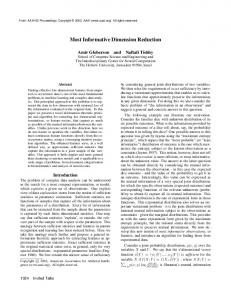
Humans are able to see objects only in 2 or 3 dimensions. However, thanks to mathematics, it is possible to design a kind of continuously evolving projections of a multivariate data cloud onto a plane. The idea was for the first time formulated by Asimov [13], who discussed the problem in extenso and proposed some algorithms how to do it in a reasonable way. The topic seemed to be attractive and was elaborated by other researchers. For the present analysis, we have chosen the method called pseudo grand tour (PGT) , which is implemented in Matlab [14,15]. Generally, the PGT method rotates the centered data cloud; after each rotation the data points are projected onto a plane with two predefined axes Z1 and Z2; and then we may observe projections of individual data points of the cloud in a scatter plot. The projections are make sequentially; after each succeeding rotation the content of the actual scatter plot is deleted and newly created points-projections are depicted. Fig. 2 shows some snapshots observed when running the PST for the considered (standardized) data set. 1
2
4
4
4
6
3
4
2
2
2
1 0 0
0
−1
−2
−2
−2 −3 −10
−5
0
5
−4 −5
0
5
5
−4 −5
0
7
8
3
4
4
2
3
3
2
2
1
1
0
0
−1
−1
−2
−2
1
5
0 −1 −2 −3 −5
0
5
−3 −5
0
5
−3 −5
0
5
Fig. 2. Snapshots from the pseudo grand tour using standardized data. Take notice that the data cloud contains two separate clusters, one smaller (group of outliers noticed for unloaded machine), the other bigger (for properly loaded machine) Fig. 2 shows clearly that the data consists of two distinct parts, which are visible in many snapshots. This fact will be explained in next section. It may be interpreted as data clusters for unloaded and loaded machine.
4
Mechatronics Systems, Mechanics and Materials 2011
Low dimensional visualization using PCA and self-associative neural network Principal component analysis (PCA)
PCA is a well established method used for reduction and low-dimensional visualization of data [16,17,4]. The dimensionality is estimated from eigenvalues of data correlation matrix using Kaiser's rule or inspecting the scree graph. Both rules indicated for our data that only the first three eigenvalues bear some relevant information, thus the dimension of the data may by reduced to dim=3. For analyzed data, the first 3 largest eigenvalues are equal to: λ1 = 6.11 , λ1 = 2.45 , λ3 = 1.02 and their sum constitutes 64% of total variance of the data. Thus, according to Kaiser's principle, the dimension of the analyzed data set is at most dim=3, and the remaining dimensions represent some noise. Each dimension is represented by a new variable called principal component. For 3 dimensions we obtain three principal components PC1, PC2, PC3 which may be displayed in the coordinate system designated by the eigenvectors associated with the first 3 largest eigenvalues λ1 , λ2 , λ3 of the data. To perform the PCA, we need an algorithm for computing eigenvalues and eigenvectors of the covariance or correlation matrix of the data vectors and specialized software performing the calculations (we have used Matlab for that purpose) [16]. Let us mention that PCA represents a purely linear approach which can locate only linear dependencies. It produces new features called principal components (PCs) which are mutually uncorrelated. Self-associative neural networks
Artificial neural networks (ANNs) are a nature inspired computing metaphor yielding another approach for solving various problems in regression and classification [18,19,4]. They are able to deal with non-linear dependencies. The basic principle for constructing an artificial neural network is simple: it builds layers of neurons, from input layer to output layer, and the input information is propagated - and reorganized - from the input through intermediate layers to the output layer which produces the desired result. Of course, this is the simplest idea describing a simple, feed forward ANN called multilayer perceptron; the ANNs may have much more complicated structure [18,19]. To get something what is similar to PCA (scores in reduced dimension of data containing compressed information on the entire data set and able to approximate the original data) we may use also ANNs. There are simple ands more sophisticated ANNs; for our investigation we have chosen a classical ANN called multi-layer perceptron (MLP) [18,19,4]. We have used a 3-layer neural network with the architecture: 15-2-15 or 15-3-15. This means that the network had input layer with 15 neurons, one intermediate layer with 2 (or 3) neurons, and output layer with 15 neurons. Let H denote the number of (hidden) neurons contained in the intermediate layer (we will consider H=2 and H=3 for a 2D and 3D visualization appropriately). During its work, the network receives at its input data vectors x = (x1, … , x15), transforms them to H scores (z1, … , zH) computed by the formula shown in eq. (1), using a system of weights {whj}:
15 z h = ϕ ∑ x j whj + wh 0 , h = 1, K , H , for hidden layer neurons, (1) j =1 with ϕ (.) denoting the tanh (tangens hyperbolicus) function. This is done by the intermediate layer of the network. The compressed values are analogues of the PC scores PC1, PC2, … , PCH obtained in PCA computations. To solve our problem, the target of the MLP (y) is defined as equal to the input data (x); therefore the number of input neurons and output neurons is the same (for our data equal to 15). To reproduce the data from the H scores, the output) layer of the network computes them from the scores z1, … , zH using another set of weights {vkh}, as shown below:
5
15 yk = ϕ ∑ z h vkh + vk 0 , k = 1, K , 15, for output layer neurons. (2) j =1 The squared difference between the input vector x and the output vector y is called squared error E: E = y − x 2 = ( y − x )T ( y − x ) (3) Obviously, the output vector y is a function of the weights {whj}, {vkh} and of the data (x) given as subsequent data vectors: y = y (x, {whj}, {vkh}) . During a process called training of the network, the weights of the neurons are accommodated to the data to make the error E as small as possible [19, 20]. Let us note that the used tanh function introduces some nonlinearity into the assumed model. 2
2D displays of the analyzed data
In first place, we will inspect the data viewed in 2 dimensions. Top left exhibit (subplot [1, 1]) in Fig. 3, subplot [1, 1], shows the scatter plot of the data obtained by PCA that is, displayed in the coordinate system of the first two principal components PC1 and PC2. The points visible in the scatter plot are in fact points-projections onto the PC plane spanned by the first two eigenvectors of the correlation matrix R of the data. They represent compressed version of all the data; it was proved that they contain the maximum amount of total variance possible to extract by two independent linear functions [16].
PCA mlp 15−2−15
6 0.6
4
0.4
0.2
0
0
Z2
PC2
2
−0.2
−2 −0.4
−4
−0.6
−6 −8
−6
−4
−2 PC1
0
2
−0.8 −0.8
4
−0.6
−0.4
−0.2
0
0.2
0.4
0.6
0.2
0.4
0.6
Z1
mlp 15−2−15
mlp 15−2−15
0.6
0.4
0.4
0.2
0.2
0
Z2
0.6
Z2
0.8
0
−0.2
−0.2
−0.4
−0.4
−0.6
−0.6 −0.8
−0.6
−0.4
−0.2
0 Z1
0.2
0.4
0.6
−0.8 −0.8
−0.6
−0.4
−0.2
0 Z1
Fig. 3. 2D displays of the analyzed data set. Top left: data points in the coordinate system of the first two principal components. Remaining exhibits: values of compressed variables Z1 and Z2 produced by a 3-layer self-associative neural network from 3 independent runs of the network
6
Mechatronics Systems, Mechanics and Materials 2011
Analogous scatter plots obtained by using scores {z1 , z 2 } produced by the self-associative neural network (MLP with the architecture 15-2-15) are shown in subplots [1,2], [2,1], and [2,2]; the exhibits show results of three independent runs of the described MLP. The results were obtained using the mlp function from the Matlab package Netlab [20]. It is amazing, how topologically similar are the displays produced by PCA and MLP. The principal components were forced to produce independent scores; the MLP was supposed to produce a pair of scores reproducing jointly as good as possible (in the assumed metric) the input data. After rotating and perhaps reflecting, the displays are nearly identical. So far all the visualization methods show clearly that the data may by subdivided into two clusters, one bigger, the other much smaller. Interpretation of data shape in reduced space
It was found that the particular shape of the data (group membership) depends on an external factor ZWE denoting load of the excavator. Fig. 3 shows a scatter plot displayed in the coordinate system of PC1 and PC2, with data vectors corresponding to small load marked in black. One may see that this is the factor responsible for the strange shape of the displayed data. PCA 6
4
PC2
2
0
−2
−4
−6 −8
−6
−4
−2 PC1
0
2
4
Fig. 4. Points-rows from the analyzed data set displayed in the coordinate system of the first two principal components. Small or no load condition is marked in black color. One may notice that the no/small load factor is determining the location of the data points. 3D visualization by PCA and MLP
Taking the first three principal components we may display them in a 3D scatter plot. This is shown in Fig. 5, subplots [1,1], [1,2] and [2,1]. All these subplots show the same data, however viewed in three different aspects. Comparing these 3D plots with the 2D plot shown in Fig. 3 one may notice that the third dimension is helpful in locating some details of the data clusters, which were not seen in the 2D plot. The main previous notice - that the data are composed from two parts - remains valid. Using the information yielded by the load factor we have marked points corresponding to small load as black points. And here again one can see clearly that just this factor separates the data into two groups: one bigger, working under charge, and the other smaller, corresponding to instances working under small or no load. Subplot [2,2] shows an analogous display obtained when using self-associative neural network (MLP) with the architecture 15-3-15.
7
Looking at that plot one may observe again the unusual shape of the analyzed data: it contains two scattered parts, which may be attributed to no/small load run (black dots) and under normal load (marked by green stars).
PCA good data
PCA good data
4
4 2
0
PC3
PC3
2
−2
−2
−4 10 5 0
PC2
−5 −10 −10 PCA good data
−10
−4 5
0 PC1
0
0 PC2
−5
PC1
−10 10 mlp 15−3−15
1
5
0.5
0
Z3
PC3
0
0
−5 5 0 PC2
−10 −5
0 −10 10
PC1
−0.5 1 1 0
0
Z2
Z1
−1 −1
Fig. 5. Some representative 3D displays of the n=951 data-points from the analyzed data set. The subplots [1,1], [1,2], [2,1] show scatter plots in the coordinate system designated by PC1, PC2 and PC3 and viewed under different aspects. Subplot [2,2] shows 3D representation yielded by the selfassociative neural network. Data points representing instances with small/no load are marked by black color.
Summary
We have considered a big real data set collected for making diagnosis of the condition of a planetary gearbox. As it was reported in previous work, diagnosis of such complex machines is difficult and require advanced both signal and data processing. In this paper, we propose to simplify the problem of multidimensional data analysis. By application of advanced data projection techniques we are able to significantly reduce observation space. In the paper different approaches have been used and for each case very similar results have been obtained. Dealing with smaller observation space it is much easier to analyze and interpret structure of data. Using multivariate visualization methods like pseudo grand tour, principal components and self-associative neural networks with 2 and 3 hidden neurons, we were able to discover an unusual shape of the distribution of the analyzed data points. The unusual shape was explained by an additional variable gathered in the experiment, which shows that the data appear as composed from two clusters, one of them being a big set of outliers. In this paper some powerful procedures have been tested for good condition data only. So, in fact, the purpose of this paper is not detailed diagnosis, but preparing data and understanding them, before proper diagnostic decision will be made. Acknowledgments
8
Mechatronics Systems, Mechanics and Materials 2011
Paper is financially supported by State Committee for Scientific Research in 2009- 2012 as research project
References
[1] [2]
[3] [4]
[5]
[6] [7]
[8] [9] [10] [11] [12]
[13] [14]
[15] [16] [17] [18]
[19] [20]
J. Antoni: Cyclostationarity by examples in Mechanical Systems and Signal Processing, 23/4, (2009), p. 987-1036 T. Barszcz, R.B. Randall: Application of spectral kurtosis for detection of a tooth crack in the planetary gear of a wind turbine in Mechanical Systems and Signal Processing, 23, (2009), p. 1352 -1365 A. Grzadziela: An analysis of possible assessment of hazards to ship shaft line, resulting from impulse load, in Polish Maritime Research, 14/3, (2007), p. 12-20 E.P. de Moura, C.R. Souto, A.A. Silva, M.A.S. Irmao: Evaluation of principal component analysis and neural network performance for bearing fault diagnosis from vibration signal processed by RS and DF analyses in Mechanical Systems and Signal Processing, 25, (2011), p. 1765 - 1772 W. Bartelmus, R. Zimroz: A new feature for monitoring the condition of gear- boxes in nonstationary operating systems in Mechanical Systems and Signal Processing, 23/5, (2009), p. 28-1534 Cz. Cempel: Multidimensional condition monitoring of mechanical systems in Operation, Mechanical Systems and Signal Processing, 17/6, (2003), p. 1291-1303 Cz. Cempel, M. Tabaszewski: Multidimensional condition monitoring of machines in nonstationary operation in Mechanical Systems and Signal Processing, 21/3, (2007), p. 12331241 W.J. Staszewski: Wavelet data compression and feature selection for vibration analysis Journal of Sound and Vibration, 211/5, (1998), p. 735-760 P.D. Samuel, D.J. Pines: A review of vibration-based techniques for helicopter transmission diagnostics in Journal of Sound and Vibration, 282/1-2, (2005), p. 475-508 R. Zimroz, W. Bartelmus: Gearbox condition estimation using cyclo-stationary properties of vibration signal in Key Engineering Materials, 413-414, (2009), p. 471-478 J. Dybala, S. Radkowski: Geometrical method of selection of features of diagnostic signals in Mechanical Systems and Signal Processing, 21/2, (2007), p. 761-779 A. Bartkowiak, R. Zimroz: Outliers in vibration signals of two planetary gearboxes working in non-stationary operating conditions - a case study 9th Int. Conf. DAMAS 2011, Univ. of Oxford, UK, in Journal of Physics: Conference Series (JPCS), (2011), in press D. Asimov: The grand tour: a tour for viewing multidimensional data in SIAM Journal of Scientific and Statistical Computing, 6, (1985), p. 128-143 E.J. Wegman, J. Shen: Three-dimensional Andrews plots and the grand tour, Proceedings of the 25th Symposium on the Interface, San Diego, Ca, in Computing Science and Statistcs, 25, (1993), p. 284-288 W. Martinez, A. Martinez: Exploratory Data Analysis with MATLAB. Chapman and Hall/CRC, Boca Raton, London (2004) I.T. Jolliffe: Principal Component Analysis. 2nd Edition, Springer, New York (2002) Q. He, R. Yan, F. Kong, R. Du: Machine condition monitoring using principal component representations in Mechanical Systems and Signal Processing, 23/2, (2009), p. 446-466 K. Worden, W.J. Staszewski, J.J. Hensman: Natural computing for mechanical system research: A tutorial overview in Mechanical Systems and Signal Processing, 25, (2011), p. 4111 C.M. Bishop: Neural Networks for Pattern Recognition. Clarendon Press, Oxford UK (1995) I.T. Nabney: Netlab, Algorithms for Pattern Recognition. 2nd printing, Springer, London (2003)