Data-Driven Depth Map Refinement via Multi-Scale Sparse ...
Recommend Documents
map especially for large depth discontinuities always cause annoying artifacts in disocclusion regions of the synthesized view. Pre-filtering approach and ...
Depth Map Fusion with Camera Position Refinement. Radim Tylecek and Radim Šára. Center for Machine Perception. Faculty of Electrical Engineering,.
a complete scene from image-based methods is a fundamental problem in ... multi-view stereo which provides rapid and accurate depth-. D. McKinnon is with ...
Wangmeng Zuo. Harbin Institute ... Zhenhua Guo, David Zhang. Hong Kong .... Zuo et al. [31] proposed a combined angular distance to combine the distances of ...
achieves higher verification accuracy than state-of-the-art palmprint recognition ..... can be efficiently done by solving one 1D minimization problem for each of its ...
Disparity Map Refinement and 3D Surface Smoothing via Directed Anisotropic Diffusion. Atsuhiko Banno. Institute of Industrial Science the University of Tokyo.
Jun 12, 2017 - [4] Bao-Di Liu, Yu-Xiong Wang, Bin Shen, Yu-Jin Zhang, and Martial Hebert. Self- ... [13] Jianchao Yang, Jiangping Wang, and Thomas Huang.
bounded by the Taormina Line (Ghisetti and Vezzani, 1982) to the southwest and by Tindari-Capo S. Alessio Alignment (Catalano et al.,. 1996) to the northeast.
Keywordsâ wavelet, adaptive filtering, SAR, speckle. I. Introduction. WITH the ... the radar backscattering coefficient cannot be derived from only one pixel ...
polarization switching device, and polarization-selective scattering screens. ..... Elements and their SoC Developments to Realize the Integrated Service System.
(a) Example of chess board image, (b) depth image of (a) without mapping of 2D image. 5. Conclusion. We have analyzed a PDDM which is useful in designing ...
The Ken Burns effect is a simple example that combines zooming and panning effects and is widely used in screen savers. For television and movie productions,.
on south and west facing windows, maintenance of heating/air conditioning ducts, replacing air filers and installing air
outlined by highly-mobile S3 twin boundary; this may provide an advantage in grain growth. Crystallo- graphic measurements have shown that the fine- grained ...
special program \E cient Algorithms for Discrete Problems and Their ... To ensure certain continuity properties of the sti ness matrix in the nite element method, .... From our algorithmic approach one can easily derive an exact algorithm as well, fo
no more possible to define the reduct of an algebra by .... Asn → As;. A is called the carrier set of the algebra. ..... booleana algebras (and for Heyting algebras).
Feb 23, 2011 - achieved at the shape signature extraction stage or after the ... binary CSS image, which is generated by the location and scale ...... Cem Direkoglu is a research fellow in Center for Digital Video Processing (School of ...
keywords (i.e., index terms) and defined a ranking function (or retrieval function) to associate a relevance degree for each document with its respective query [1,.
coding theorem, the MDC admissibility of the ( M + L)- tuple (RI.. . RM,~.. .O), (i.e., with arbitrary small error rate) depends only on the entropies hl = H(X), 1 = 1.
the existence of an integrable solution to the refinement equation is obtained by considering .... To see that (a) and (a') are equivalent, assume that P(γ0) = 0 but ... Then E is the boundary and exterior of the ellipse shown in Figure 1. We apply
the minimum grain size attainable by these meth- ods is frequently larger than 0.1 m [11,12] and thus the development of new, more effective approaches.
Apr 29, 2007 - âMathematics Department, Smith College, Northampton, MA 01063. Email: [email protected]. â Department of Computer Science, ...
then-dense pose alignment [2]. Thus, as a future step, we might consider to integrate DL-based pose estimation into our frame stitching module to decrease the ...
Data-Driven Depth Map Refinement via Multi-Scale Sparse ...
proach is to take advantage of a training set of high-quality depth data and .... [12] defined the neighbor term using an auto- .... 2: At the coarsest level, repair y0.
Abstract Depth maps captured by consumer-level depth cameras such as Kinect are usually degraded by noise, missing values, and quantization. In this paper, we present a datadriven approach for refining degraded RAW depth maps that are coupled with an RGB image. The key idea of our approach is to take advantage of a training set of high-quality depth data and transfer its information to the RAW depth map through multi-scale dictionary learning. Utilizing a sparse representation, our method learns a dictionary of geometric primitives which captures the correlation between high-quality mesh data, RAW depth maps and RGB images. The dictionary is learned and applied in a manner that accounts for various practical issues that arise in dictionarybased depth refinement. Compared to previous approaches that only utilize the correlation between RAW depth maps and RGB images, our method produces improved depth maps without over-smoothing. Since our approach is data driven, the refinement can be targeted to a specific class of objects by employing a corresponding training set. In our experiments, we show that this leads to additional improvements in recovering depth maps of human faces.
1. Introduction The recent popularity of consumer-level depth cameras such as Kinect has led to growing interest in using depth maps as auxiliary data for various computer vision tasks, such as pose recognition [1] and scene understanding [2]. The benefits of utilizing depth data, however, are limited by the relatively low resolution of depth maps as well as depth degradations due to noise, missing values, and quantization, which can significantly reduce data quality. To facilitate the use of depth data, most methods have focused on the depth upsampling problem, in which a higherresolution depth map is recovered from a lower-resolution input. This task is typically performed with the help of a corresponding high-resolution RGB image of the scene, which is jointly captured with the depth map by Kinect. These methods make use of the RGB image through the
statistical co-occurrence of its discontinuities with those in the depth map, as they both arise from common underlying 3D structure. Since the RGB image is at a higher resolution, its discontinuities are used to locate depth discontinuities at a higher resolution than the input depth map. Many successful results have been demonstrated with this approach, but the computed depth maps often exhibit distortions and over-smoothing due to the aforementioned degradations in depth measurements. In this paper, we present a data-driven approach for dealing with the problem of low-quality depth data. The key idea is to transfer high-quality depth map primitives to the RAW depth map through multi-scale dictionary learning. Dictionaries are formed through structure-guided sparse coding [3] of RGB images, RAW depth maps, and high-quality depth data constructed by Kinect Fusion [4]. Learning the statistical relationship between low- and highquality depth maps allows our method to account for the various degradations that can occur in depth map measurement. However, there exist three major issues that complicate this approach in practice, namely RGB textures uncorrelated with depth map discontinuities, large dictionary size, and differences in geometric features at different scales. We present adaptations of our dictionary-based framework to address these practical issues in the depth refinement process. The performance of our algorithm is evaluated and compared with state-of-the-art depth map refinement methods that also take a single RGB-D image as input. Our approach consistently outperforms previous techniques both quantitatively in synthetic examples and qualitatively in real-world instances. We additionally demonstrate that by learning a class-specific dictionary, the effectiveness of our datadriven approach can be further enhanced.
2. Related work Related works on depth map refinement are reviewed in this section. These techniques can be classified as either RGB-D based techniques that utilize an additional RGB image to guide the depth map refinement process, or reconstruction based techniques that merge multiple unaligned
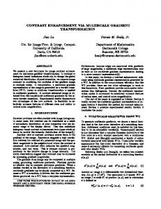
Low Quality Depth RGB
Depth High Quality Depth
(a) Slanted texture (b) 3D edge Figure 1. Practical issues. (a) Surface texture uncorrelated with depth discontinuities. (b) Variations in depth map degradation: (Top) missing depth values; (Bottom) blurred depth readings. Because of such variations, building a dictionary that couples the high- and low-quality depth map would lead to large dictionary size. (Figure adapted from [5].)
low-quality depth maps to reconstruct a high-quality depth surface. Our approach fits into the first category, which is the focus of the review presented here. RGB-D based techniques generally assume that there exists a joint occurrence between depth discontinuities and RGB image edges. Most early works make use of this assumption by adaptively filtering the depth map according to edges in the RGB image. In [6], an MRF formulation for depth map upsampling is introduced with the data term computed from the depth map and weights for the smoothness terms derived from the high-resolution RGB image. In [7, 8], a joint bilateral filter [9] is applied to fill holes and upsample a depth map with the weight of the range kernel defined by intensity differences in the RGB image. Favaro [10] introduced the nonlocal structure filter which demonstrates better structure preservation than the bilateral filter for depth map recovery. More recently, several methods have posed RGB-D depth refinement as a constrained optimization problem. Park et al. [11] formulated the depth map upsampling problem as a weighted least squares optimization with a neighbor term defined by structures in the RGB image. Yang et al. [12] defined the neighbor term using an autoregression model. Liu et al. [13] evaluated pixel dissimilarities based on geodesic distance instead of Euclidean distance to achieve sharper depth boundaries. Also, Yu et al. [14] and Han et al. [15] presented shape-from-shading based methods for depth map geometry refinement. Dictionary learning based methods have long been adopted for image restoration, in particular for denoising and hole filling [16], with high performance compared to filter-based techniques. For depth map upsampling, Kiechlel et al. [17] and Tosic and Drewes [5] presented dictionary-based methods that learn statistical dependencies between intensity and depth in a scene that naturally arise from their common underlying 3D features. With the learned dictionary, a high-resolution depth map consistent with the high-resolution image is then inferred from the low-resolution depth map. This approach, though effective with clean depth maps, can exhibit reduced performance
with depth maps containing typical measurement degradations, whose depth distortions unbalance the natural statistical dependencies. To address this problem, our method learns the statistical relationship between high-quality depth, low-quality depth and image intensity. By jointly accounting for highquality and low-quality depth, our work is able to capture and model the depth degradation, in contrast to [17, 5]. Dictionaries for these three quantities are also learned in [18]. However, the method in [18] does not address the practical issues described in the previous section. It does not include a mechanism to deal with RGB textures uncorrelated with depth discontinuities, which can mislead dictionary-based approaches. It also does not employ a technique for managing dictionary size, instead just using a fixed-size dictionary with limited performance. Our work additionally differs by learning scale-dependent and class-specific dictionaries which can elevate accuracy. Reconstruction based techniques directly estimate a higher-quality 3D model by merging multiple lower-quality depth maps captured from different viewpoints of the same scene. A state-of-the-art reconstruction-based method is Kinect Fusion [4], which aligns multi-view depth maps into a pre-allocated volumetric representation. It has been shown to be effective for modeling objects with a volume within a few cubic meters [19]. Although reconstruction based techniques generally produce higher-quality 3D data than RGB-D based methods, they are more practical for static scenes than for dynamic environments. Through this approach, several research groups have utilized Kinect to build RGB-D datasets [20, 21] of various scenes and objects for scene categorization, object recognition and segmentation. Since Kinect depth maps, as well as depth maps from other consumer-level depth cameras, often contain holes and other measurement degradations, depth map refinement is beneficial for downstream vision tasks.
3. Practical Issues In this section, we discuss the three major practical issues and how they can affect the quality of recovered depth maps. The first issue exists for all previous algorithms that utilize RGB edges to guide depth map refinement. The second and third issues affect methods based on dictionary learning. Uncorrelated texture and depth discontinuities. Although discontinuities in RGB images and depth maps often coincide due to common scene structure, this is frequently not the case because of surface textures whose intensity variations are independent of depth, as illustrated in Figure 1(a). Consequently, defining depth smoothness weights based on RGB image gradients can lead to texture copying artifacts in the resulting depth map. Even when RGB edges
and depth discontinuities co-occur, the gradient magnitudes of RGB edges depend on intensity differences between the two depth layers, not on depth differences. As a result, edge sharpness in the refined depth map may be affected by surface colors, such that a sharp boundary between two depth layers may exhibit edge sharpness variations due to textures. Large dictionary size. In image restoration, the degradation process is assumed to be uniform across the entire image. However, as illustrated in Figure 1(b), this assumption does not hold for the depth map recovery problem where a given local scene region can be measured as different lowquality depth patches due to different forms of degradation, such as missing values (e.g. from the disparity problem in Kinect), quantization, noise (e.g. depth-dependent ToF noise), and blur (e.g. from ToF imaging). To account for such variations in modeling the statistical relationship between low- and high-quality depth maps, the size of the dictionary would need to be expanded dramatically. In [18], the fixed-size dictionary limits the ability to model the various depth map degradations, hence curbing the performance of the method. Scale-dependent depth features. Dictionaries learned at a certain geometric scale may not be as suitable at another scale due to differences in geometric features. Taking human faces as an example, dictionary primitives may model the shapes of facial features such as the nose and cheeks at one level, but primitives that capture skin details such as wrinkles would be more useful at a finer scale. Thus, using a dictionary learned at one scale for refining depth maps at another can be less effective.
4. Proposed Algorithm As in other dictionary-based depth refinement methods, ours assumes that local patches in depth maps and RGB images can be represented by a sparse linear combination of basis functions [22]: y = Dα,
(1)
where y = {yh , yl , yc } denotes the high-quality depth map, low-quality RAW depth map, and aligned RGB image respectively, D = {Dh , Dl , Dc } denotes their corresponding dictionaries containing basis functions, and α = {αh , αl , αc } represents sparse vectors of basis function coefficients. Our goal in this work is to recover yh given yl and yc , by learning a joint dictionary of {Dh , Dl , Dc } such that αh = αl = αc : yh Dh arg min yl = Dl α + λ|α|1 , (2) D,α yc Dc where |α|1 is the L1 -norm of α, and λ is a parameter to control the sparsity of coefficients. Using the learnt joint
(a) RGB Image (b) Raw Image (c) Single scale (d) Multi-scale Figure 3. Results from single and multi-scale dictionary recovery, shown as RGB texture mapped onto a depth surface. The dark lines and regions result from depth quantization and missing data due to occlusion.
L0 -RGB Raw depth 1st level 2nd level 3rd level Figure 4. Multi-scale refinement of the depth map. 1st: coarsest level; 2nd: middle level; 3rd: finest level. For illustration, the depth maps in the 1st and 2nd levels are bicubic upsampled to the resolution of the 3rd level.
correlation in {Dh , Dl , Dc } from training data, we first estimate the α which minimizes yl = Dl α and yc = Dc α. We then use Dh and the estimated α to recover yh = Dh α. This framework follows standard procedures in dictionarybased image restoration [16] and super-resolution [23]. We refer readers to [23] for details on joint dictionary learning and sparse coefficient estimation [24]. In the following, we describe our main contributions on how to address the three practical issues within this dictionary-based framework. RGB-D structure similarity measure. To deal with the first issue of uncorrelated texture and depth discontinuities, we formulate a measure for predicting which RGB edges are most likely to coincide with depth discontinuities. To determine this reliably, we examine the consistency between local edge structures and depth layer boundaries, rather than simply taking the gradient magnitude of individual pixels. After upsampling the depth map by bicubic interpolation to the resolution of the RGB image, the similarity measure is computed as follows: κ(yl (x), yc (x)) =
where g(yl (x)) = {∂x yl (x0 ), ∂y yl (x0 )}, x0 ∈ N (x), is a concatenation of gradients in the x (∂x ) and y (∂y ) directions within a local neighborhood N (x) of x, < ·, · > denotes the dot product operation, | · | denotes the absolute value operator, and k·k2 is the Euclidian norm of a vector. In our implementation, N (x) is defined as a 3 × 3 local neighborhood, g(yc (x)) is defined using the maximum gradient magnitudes among the RGB channels, and κ(yl (x), yc (x)) is set to zero if either kg(yl (x))k2 or kg(yc (x))k2 is smaller
(a) Color (b) nAGDP (finest level) (c) without nAGDP (d) with nAGDP (e) Ground Truth Figure 2. The normalized Absolute Gradient Dot Product (nAGDP), which identifies RGB edges most likely to coincide with depth discontinuities (where the red end of the spectrum indicates higher values, and the blue end represents lower values). Dictionary-based depth map refinement based on Equation (5) using nAGDP exhibits improvements over refinement without it (κ = 1). In this example, the RAW depth map is upsampled by 8×.
than a threshold. We refer to this measure as the normalized Absolute Gradient Dot Product (nAGDP). Figure 2(b) shows an example of our nAGDP map, which effectively indicates RGB edges that coincide with depth discontinuities. We utilize the nAGDP map to guide the depth map refinement process as described later. The effect of κ on depth map refinement is illustrated by the comparison in Figure 2(c) and (d), which exhibit dictionary-based refinement without and with nAGDP, respectively. Multi-scale solution to address degradation variation. Since the variations in depth degradation lead to considerably more triples among low-quality depth, high-quality depth, and intensity, the number of dictionary primitives needed to model them would increase considerably. Representing this with only a fixed dictionary size as in [18] would result in inadequate performance. Our solution to this problem is to reduce the effects of degradation variation via a multi-scale solution where degradation effects are significantly reduced at coarser scales, and refinement solutions at coarser scales are used as a proxy for the low-quality depth patches at finer scales. By learning dictionaries using these proxies instead of the original low-quality depth map, we circumvent the issue of degradation variation on dictionary size. To train our dictionary, we downsample the training data by a factor of 8 using bicubic interpolation. The downsampling reduces degradation effects like noise, holes and quantization in yl , while yh and yc remain accurate after downsampling. If missing values exist after downsampling because of large holes, they are filled by using the method in [11]1 . The hole filling of [11] may produce texture copying artifacts and inaccurate depth boundaries due to irrelevant image gradients in the RGB image. To avoid this, we modify their smoothness term by setting its weight equal to (1 − κ) and use only the first order neighborhood for depth propagation within the hole regions. Applying the hole filling on the downsampled depth map rather than at the original resolution minimizes bias from the hole filling 1
Source code at http://rcv.kaist.ac.kr/˜jspark/ projects/high_quality_depthmap_upsampling/
Algorithm 1: Dictionary Learning Input: yh , yl , yc Output: Dh ,Dl ,Dc 1: Create Gaussian pyramid of yh , yl , yc 2: At the coarsest level, repair yl0 using [11] 3: Bicubic downsample repaired yl0 to get y ˜l0 4: For each i-th level, do: 5: Compute κ using Equation (3) 6: Learn {Dih ,Dil ,Dic } using Equation (4) 7: Reconstruct yhi using Equation (6) and (7). 8: Set y˜li+1 = yhi 9: Output Dh ,Dl ,Dc at each level Algorithm 2: Depth Map Refinement Input: yl , yc , Dh ,Dl ,Dc Output: yh 1: Create Gaussian pyramid of yl , yc 2: At the coarsest level, repair yl0 using [11] 3: Bicubic downsample repaired yl0 to get y ˜l0 4: For each i-th level, do: 5: Compute κ using Equation (3) 6: Reconstruct yhi using Equation (6) and (7). 7: Set y˜li+1 = yhi 8: Output reconstructed yh at the finest level method. After hole filling, we further downsample yl by 2× to obtain the proxy solution at the coarsest resolution, y˜l0 . Scale-dependent dictionaries. Using the proxy solution, y˜l0 , and the downsampled yh0 and yc0 , we can learn a dictionary and use it to reconstruct and upsample the depth map progressively up to the original resolution of the RGB image. However, this would ignore the differences in geometric features that occur at different scales. We therefore learn a dictionary at each level of the multi-scale solution. To learn the dictionary at a level i, we solve the following minimization problem: i i 2 y Dh h i i i y˜l − Dl α + λ|αi |. (4) arg min Di y´ci Dic
Instead of using yci directly, we filter yci with L0 -norm smoothing [25] to enhance sharp edges and reduce image noise. After that, we convert the filtered yci to a gradient image and keep only the maximum magnitude among the RGB channels. Within each image patch, gradients are then normalized by the maximum gradient magnitude to yield y´ci for training. These steps are taken because gradient magnitude and direction are uncorrelated with depth map discontinuities. In our implementation, we use patches of size 8×8 for yhi and yci , and size 4 × 4 for the lower-resolution y˜li . Depth patches are normalized to have zero mean before training. At each level, we randomly sample 100,000 patches from a training set with a higher probability for patches that contain a larger local sum of κ. After training, each Dih , Dil , Dic contains 1024 patches (basis functions) coupled among the dictionaries. The dictionary learning algorithm is summarized in Algorithm 1, and the effects of multi-scale dictionary learning and progressive refinements are demonstrated in Figure 3 and Figure 4 respectively. Depth map refinement. To refine the low-quality input depth map, we first estimate the sparse reconstruction coefficients of patches by minimizing the following function: arg min k˜ yli − Dil αi k2 + κk´ yci − Dic αi k2 + λ|αi |. (5) i α
In order to ensure consistent reconstruction between neighboring patches, we modify Equation (5) by considering overlapping patches. For each patch, the sparse coefficients are then estimated by minimizing arg min P(x)kyhi (x) − Dih αi (x)k2 + k˜ yli (x) − Dil αi (x)k2 i α (x)
+κ(x)k´ yci (x) − Dic αi (x)k2 + λ|αi (x)|,
(6)
where P(x) is a binary mask that indicates parts of the reconstructed depth map that lie within patch overlap areas. By incorporating the nAGDP map, κ, into Equation (6), we avoid irrelevant edges in the RGB image which can mislead coefficient estimation. In our implementation, the refined patches overlap by a 6-pixel margin. Depth patches are refined in descending order of the local sum of κ. For patches with the same κ sum, the ordering is determined based on the amount of overlap with patches that have a higher κ sum. This ordering allows reliable patches along depth discontinuities to be reconstructed before patches in interior regions [26]. Finally, using the estimated coefficients αi for patches over the entire image, we reconstruct the depth map by solving the following optimization function: X X i arg min ky (x) − w(x0 )Dih αi (x0 )k2 h i yh
x0
x
X +µ (1 − κ(x))|∇yhi (x)|, x
(7)
P where x (1 − κ(x))|∇yhi (x)| is the total variation regularization weighted by (1−κ(x)) which suppresses P noise in reconstruction, w(x0 ) is a blending function ( x0 w(x0 ) = 1) for overlapping patches which is defined according to distance from the patch center, and µ = 0.1 in our implementation. The refinement procedure is summarized in Algorithm 2.
5. Experiments We first compare our method with state-of-the-art techniques for depth map upsampling using the noisy Middlebury dataset from [27]. Then, we evaluate the performance of our method on depth map completion and enhancement using a public Kinect dataset [21] and a ToF dataset [27]. Finally, we demonstrate our data-driven recovery using class-specific dictionaries on face data. Additional results, including a computation time comparison, quantitative comparisons using a clean Middlebury dataset [29], qualitative comparisons with various Kinect scene datasets, and three videos each of recovered Kinect/ToF face depth and ToF scene depth mesh models are provided in the supplemental material. We assume that the training and testing data are captured at the same scale. For objects such as human faces, scale normalization can be done through a face detector.
5.1. Training data collection In collecting training data, we employ Kinect Fusion [4] to capture high-quality mesh data as shown in Figure 5. We also record camera poses, RAW depth maps, and corresponding RGB images. The high-quality and low-quality depth map pair is obtained through projection of the captured mesh data and RAW depth map after geometric alignment to the RGB image. In the training process, different levels of the multiscale dictionary learning are separated by a scale factor of dlog2 M e, where the magnification M is the ratio between the resolution of the RGB image and RAW depth map. The number of scales and patch sizes were set empirically based on the SNR of depth maps. In our experiments, we found that three levels are suitable for natural scenes, and two levels are sufficient for face data. We have tested the face data with a three-level multiscale dictionary, but the results were similar to that of two levels. Thus, we chose two levels to reduce computation time. As for patch size, a larger patch has a greater space of variation and thus requires a larger dictionary as well as more computation. A smaller size of patches in low-quality depth maps is preferable because the greater noise in a low-quality depth map would otherwise result in a large dictionary. As for the selection of training data, since we do not have any prior knowledge about the structures in a given scene, we gather training data that contains a rich variation in geometry.
(a)
(b)
(c)
(d)
Figure 5. Training data examples. Top row: a natural scene; Bottom row: a human face. (a) Kinect Fusion mesh, (b) High-quality depth map from projected mesh, (c) RAW depth map, (d) RGB image (after L0 -norm smoothing for natural scenes). Table 1. Upsampling of noisy Middlebury dataset
2× Park et al.[11] 3.76 Ferstl et al.[27] 3.19 Kiechle et al.[17] 2.82 3.02 Li et al. [18] Ours(w.o. nAGDP) 0.99 Ours(w. nAGDP) 0.87
Table 2. ×8 Upsampling of noisy Middlebury dataset Art Books Moebius Planar Dict. 5.34 Ours 2.05
1.19 1.14
2.44 1.37
5.2. Noisy Middlebury dataset We apply our algorithm to the depth map upsampling problem using the noisy Middlebury dataset provided by [27]2 . In this experiment, our multi-scale dictionary is trained from our Kinect examples for natural scenes. We progressively upsample and refine the recovered depth map by a factor of 2× until the depth map resolution reaches the target upsampling resolution. Table 1 reports quantitative comparisons to related methods in terms of RMSE, and Figure 6 shows a qualitative comparison of 8× upsampling for the Art example. The training data used for the state-of-theart learning-based approach [17]3 are identical to that used for our method. Comparisons are also presented for our approach without and with nAGDP . Our approach consistently outperforms the compared methods4 , indicating that 2 https://rvlab.icg.tugraz.at/project_page/ project_tofusion/project_tofsuperresolution.html 3 Source code from http://www.gol.ei.tum.de/index. php?id=6&L=1 4 q Note that the standard RMSE used in Table 1, e.g. RM SE(θ) = E((θˆ − θ)) where θˆ is the upsampled result and θ is ground-truth, is different from the metrics used in [27] and [17]. Comparisons with other
our dictionary representation learnt with Kinect data is effective and general enough for refinement of non-Kinect depth degradations. In Table 2, we show results for an additional experiment where the training data contains only large planar objects. Using training data with large planar objects is effective for scenes composed of planar surfaces, but results in larger error for scenes with curved surfaces and regions with small scale geometry.
5.3. Kinect natural scene data We also tested our algorithm on natural scene data in Figure 7, where the first two examples are from the NYU RGB-D dataset [21] and the last one is from Park et al. [30] which has ground truth depth from Kinect Fusion. More examples can be found in the supplemental material. We compare our results with those from Park et al. [11], Kiechle et al. [17], and Li et al. [18]. Our results exhibit higher-quality refinement especially for regions with ambiguities. In Figure 7(d), although our results are less sharp, our refined edge locations are more accurate due to the usage of nAGDP. For the third example, we provide RMSE values in addition to difference maps between ground truth and results, which indicate the effectiveness of our method quantitatively. The use of nAGDP helps our approach to avoid irrelevant RGB error metrics are presented in the supplemental material.
(a) RGB
(b) Input
(c) Park et al.[11] (d) Ferstl et al.[27](e) Kiechle et al.[17](f) Ours (w. nAGDP) Figure 6. Examples of 8× upsampling on the Art dataset.
100 90 80 70 60 50 40 30 20 10 0
(a) RGB
Grond-truth (b) RAW
RMSE: 7.16 (c) Park[11]
RMSE: 6.64 (d) Kiechle[17]
RMSE: 7.27 (e) Li [18]
RMSE: 5.76 (f) Ours
Figure 7. Comparisons on natural scene data captured by Kinect. More examples can be found in the supplemental material.
edges and bleeding of depth map values. The multi-scale processing also plays an important role in correctly refining the depth map at different scales.
5.4. ToF dataset We additionally tested our method on the real-world ToF dataset provided by [27], with ground truth depth maps obtained using a structured light scanner. An example of our results is shown in Figure 8, along with a quantitative comparison.
5.5. Kinect face data In Figure 9, we demonstrate our method on class-specific depth refinement using human faces. Our face dictionary is trained at multiple scales using six faces whose high-quality depth maps were captured with Kinect Fusion. The face areas are manually cropped and resized to the same scale for both training and testing. As shown in Figure 9, the RAW depth maps are full of quantization errors and have missing depth values around the nose due to occlusion. Our results are compared with those of Kiechle et
Books Devil Shark RMSE[mm] RMSE[mm] RMSE[mm] He et al.[28] 14.90 15.74 14.08 Ferstl et al.[27] 6.5 8.42 7.74 7.1 5.81 8.8 Ours(w.o. nAGDP) Ours(w. nAGDP) 4.02 3.56 5.5 Bold text indicates the best result.
Figure 8. Real-world ToF data upsampling. Left: Y-channel image, and upsampled depth map. The RAW low-resolution depth map is shown in the upper-left corner of the output depth map (relative resolution between the two images is preserved). Right: RMSE comparison.
Front view
(a) RGB
(b) RGB crop
(c) RAW
Side view
(d) Kiechle[17]
(e) Ours
Figure 9. 3D meshes of face testing examples. Side views are arranged in the same order as the front views.
al. [17], for which the aligned Kinect Fusion depth map is used to train their joint intensity and depth co-sparse dictionary. Different from our method, theirs does not include low-quality depth maps as training data, and their reconstruction is performed at a single scale. For better visualization, we also show side views of recovered depth maps. Note that our method does not over-smooth the sharp features of noses and mouths. We also note that the shape of the nose in the third example of our results is different from the actual nose shape. This is because the large quantization errors introduce ambiguities in dictionary matching, which cannot be resolved using only the given frontal view. The benefit of using multi-scale and data-dependent dictionary learning is illustrated in Figure 10. In (b), the results are generated using a generic multi-scale dictionary trained from natural scenes. In (c), the depth maps are computed using the same dictionary at each scale, which was learned from faces. Results of our proposed approach, with different dictionaries learned for different scales from face data, are exhibited in (d). Even though we applied the same multi-scale approach to each case, the outcomes are different according to the dictionaries used. The most severe case is the generic dictionary which results in over-smoothing across the entire facial structure. With the same face dictio-
(a)
(b)
(c)
(d)
Figure 10. Different dictionaries for face reconstruction with the multi-scale approach. (a) RGB; (b) Generic dictionaries; (c) Single dictionary for different levels; (d) Ours.
nary at each scale, critical facial features are over-smoothed, such as at the tip of the nose. These distortions indicate that a single dictionary does not adequately model face geometry at different scales. For experiments on ToF face data, please see the supplemental material.
6. Conclusion We presented a multi-scale dictionary-based depth map refinement method that addresses three important practical issues neglected in previous work. Through modifications of the dictionary learning and reconstruction framework to deal with these matters, significant improvements in performance are gained over state-of-the-art techniques.
References [1] J. Shotton, A. Fitzgibbon, M. Cook, T. Sharp, M. Finocchio, R. Moore, A. Kipman, and A. Blake. Real-time human pose recognition in parts from a single depth image. In CVPR, 2011. 1 [2] V. Vineet, C. Rother, and P. Torr. Higher order priors for joint intrinsic image, objects, and attributes estimation. In NIPS, 2013. 1 [3] H. Lee, A. Battle, R. Raina, and A. Y. Ng. Efficient sparse coding algorithms. NIPS, 19:801, 2007. 1 [4] S. Izadi, D. Kim, O. Hilliges, D. Molyneaux, R. Newcombe, P. Kohli, J. Shotton, S. Hodges, D. Freeman, A. Davison, and A. Fitzgibbon. Kinectfusion : Real-time 3d reconstruction and interaction using a moving depth camera. In 24th annual ACM symposium on User interface software and technology, ser. UIST ’11, pages 559–568, 2011. 1, 2, 5 [5] I. Tosic and S. Drewes. Learning joint intensity-depth sparse representations. IEEE Trans. on Image Processing, 23(5):2122–2132, 2014. 2 [6] J. Diebel and S. Thrun. An application of markov random fields to range sensing. In NIPS, 2005. 2 [7] Q. Yang, R. Yang, J. Davis, and D. Nistr. Spatial-depth super resolution for range images. CVPR, pages 1–8, 2007. 2 [8] J. Zhu, L. Wang, R. Yang, and J. Davis. Fusion of timeof-flight depth and stereo for high accuracy depth maps. In CVPR, 2008. 2 [9] J. Kopf, M. F. Cohen, D. Lischinski, and M. Uyttendaele. Joint bilateral upsampling. ACM Trans. on Graph., 26(3):96, 2007. 2 [10] P. Favaro. Recovering thin structures via nonlocal-means regularization with application to depth from defocus. In CVPR, 2010. 2 [11] J. Park, H. Kim, Y.-W. Tai, M.S. Brown, and I. Kweon. High quality depth map upsampling for 3d-tof cameras. ICCV, pages 1623–1630, 2011. 2, 4, 6, 7 [12] J. Yang, X. Ye, K. Li, and C. Hou. Depth recovery using an adaptive color-guided auto-regressive model. ECCV, pages 158–171, 2012. 2 [13] M.Y. Liu, O. Tuzel, and Y. Taguchi. Joint geodesic upsampling of depth images. CVPR, pages 169–176, 2013. 2 [14] L. F. Yu, S. K. Yeung, Y. W. Tai, and S. Lin. Shading-based shape refinement of rgb-d images. In CVPR, pages 1415– 1422, June 2013. 2 [15] Y. Han, J.-Y Lee, and I.S. Kweon. High quality shape from a single rgb-d image under uncalibrated natural illumination. In ICCV, 2013. 2 [16] M. Elad and M. Abaron. Image denoising via sparse and redundant representations over learned dictionaries. IEEE Trans. on Image Processing, 15(12):3736–3745, 2006. 2, 3 [17] M. Kiechle, S. Hawe, and M. Kleinsteuber. A joint intensity and depth co-sparse analysis model for depth map superresolution. ICCV, 2013. 2, 6, 7, 8
[18] Y. Li, T. Xue, L. Sun, and J. Liu. Joint example-based depth map super-resolution. ICME, pages 152–157, 2012. 2, 3, 4, 6, 7 [19] S. Meister, S. Izadi, P. Kohli, M. H¨ammerle, C. Rother, and D. Kondermann. When can we use kinectfusion for ground truth acquisition? In Workshop on Color-Depth Camera Fusion in Robotics, IROS, 2012. 2 [20] A. Janoch, S. Karayev, Y. Jia, J. T. Barron, M. Fritz, K. Saenko, and T. Darrell. A category-level 3-d object dataset: Putting the kinect to work. In ICCV, 2011. 2 [21] N. Silberman, D. Hoiem, P. Kohli, and R. Fergus. Indoor segmentation and support inference from rgbd images. In ECCV, 2012. 2, 5, 6 [22] D.L. Donoho. Compressed sensing. IEEE Trans. on Information Theory, 52(4):1289–1306, 2006. 3 [23] J. Yang, Z. Wang, Z. Lin, S. Cohen, and T. Huang. Coupled dictionary training for image super-resolution. IEEE Trans. on Image Processing, 21(8):3467–3478, 2012. 3 [24] J. Zheng, Z. Jiang, P. J. Phillips, and R. Chellappa. Crossview action recognition via a transferable dictionary pair. In bmvc, volume 1, page 7, 2012. 3 [25] L. Xu, C. Lu, Y. Xu, and J. Jia. Image smoothing via l0 gradient minimization. ACM Trans. on Graph., 30(6):174, 2011. 5 [26] J. Sun, L. Yuan, J. Jia, and H. Y. Shum. Image completion with structure propagation. ACM Trans. on Graph., 24(3):861–868, July 2005. 5 [27] D. Ferstl, C. Reinbacher, R. Ranftl, M. Rther, and H. Bischof. Image guided depth upsampling using anisotropic total generalized variation. ICCV, 2013. 5, 6, 7, 8 [28] K. He, J. Sun, and X. Tang. Guided image filtering. IEEE Trans. on PAMI, 35(6):1397–1409, 2013. 8 [29] D. Scharstein and R. Szeliski. High-accuracy stereo depth maps using structured light. In CVPR, pages 195–202, June 2003. 5 [30] J. Park, H. Kim, Y.-W. Tai, M. S. Brown, and I. Kweon. High quality depth map upsampling and completion for rgb-d cameras. IEEE Transactions on Image Processing, 23(12):5559–72, Dec 2014. 6