Data-Driven Modelling of Wind Turbines

2011 American Control Conference on O'Farrell Street, San Francisco, CA, USA June 29 - July 01, 2011

Data-Driven Modelling of Wind Turbines Gijs van der Veen, Jan-Willem van Wingerden and Michel Verhaegen

advantage. The proposed identification method basically involves a twostep procedure. In a first step, a theoretical prediction of the aerodynamic characteristics (such as the torque coefficient) is used to choose a suitable set of radial basis functions that can be used to describe it. In a second step, standard LTI system identification is performed to retrieve the linear, timeinvariant portion of the dynamics and the coefficients of the basis functions. First, the problem definition is introduced in section II. Then, in sections III and IV the method is described in more detail. In section V the method is applied to a simulation example. The paper ends with a number of conclusions and suggestions for future work.

Abstract— In this paper we present a novel approach that allows global modelling of the power control dynamics of a wind turbine based on measured data. The approach is based on the assumption that all the nonlinearities over the operating range arise from a static aerodynamic mapping, which is interconnected with linear, time-invariant dynamics. This socalled Hammerstein structure is exploited to simplify the model identification procedure. The global model is suited to control design methods such as model predictive control or can be used to extract local linear models. The approach is demonstrated on a benchmark example, the 5 MW NREL/Upwind reference turbine and is shown to work well. Tools from convex optimisation and the recently introduced nuclear norm techniques prove to be instrumental to the successful implementation of the algorithms.

I. INTRODUCTION

II. PROBLEM STATEMENT

Current controllers for power regulation in wind turbine applications are all based on PID feedback or related methods. It is common practice to design such controllers based on linear models [1], [2]. To deal with the timevarying dynamics of the system, gain scheduling is often employed on the controller gains by which the controller is tuned in several discrete operating points and the gains are interpolated during operation. In this paper we introduce a procedure to identify a globally valid model of the dynamics of a wind turbine involved in power production [3]. Such a model can be used to extract local-linear models in several operating points, but also to design a controller that deals intrinsically with the time-varying dynamics. Furthermore, such a model has value in fault detection applications and it results in an estimate of the true torque curve of a wind turbine. In the wind energy community, linear models are usually obtained from aeroelastic models or, more recently, derived from measurement data [4], [5], with the advantage of not having to rely on the theoretical approximations made in first-principles models. In recent years, advances have been made in identification of linear parameter-varying models of wind turbines [6]. Such methods, however, are still severely hampered by computational complexity issues. For this reason, we introduce a method to identify a global model of a wind turbine that can easily cope with large amounts of sampled data. Whereas pure LTI identification of wind turbines from operational data is made difficult by a constant need to maintain a steady operating point, this is no longer necessary for the proposed method, which is another

The power production control loop of a wind turbine is commonly designed around the dynamics governed by the pitch angle β, rotor speed Ω and generator torque Tg . This is shown schematically in Fig. 1. The rotor speed can be controlled by adjusting the demanded generator torque and by adjusting the pitch angles of the blades. R V λ

Ta Wind turbine (LTI)

Ω

Tg

Fig. 1. Schematic showing a typical model of a wind turbine between pitch angle β, generator torque Tg and rotor speed Ω.

CQ (λ, β)

λ

10 8

0.06

6

0.04

4

0.02

2 −5

This work was supported by Vestas Wind Systems A/S The authors are with the Delft Center for Systems and Control, Delft University of Technology, 2628 CD, The Netherlands {G.J.vanderVeen, J.W.vanWingerden, M.Verhaegen}@tudelft.nl

978-1-4577-0079-8/11/$26.00 ©2011 AACC

f (λ, β, V 2 )

β V

Fig. 2.

72

0

5 10 15 20 β, ◦

0

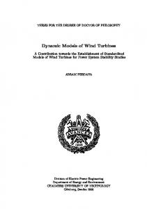
Typical shape of the torque coefficient CQ (λ, β).

Referring to Fig. 1, the aerodynamic torque Ta on a wind turbine under steady operating conditions can be described in terms of the torque coefficient CQ (λ, β) which appears in Eq. (1). 1 (1) Ta = f (λ, β, V 2 ) = ρπR3 CQ (λ, β)V 2 , 2 where Ta is the aerodynamic torque, λ is the tip speed ratio, β is the pitch angle, ρ is the air density, V is the wind speed, R is the rotor radius and CQ (λ, β) is a smooth surface (Fig. 2) depending on the pitch angle β and the tip-speed ratio λ = (ΩR)/V . The aerodynamic torque further depends on the wind speed V , the rotor radius R and the air density ρ. It is clear that the dynamics of the wind turbine subject to the aerodynamic torque in Eq. (1) are non-linear. We wish to identify a non-linear dynamic model of this system on the basis of input and output measurements obtained from the system operating in closed-loop, based on a set of measurements {uk , yk }N k=1 . The system to be identified is assumed to admit an innovation state-space representation given by: xk+1 = Axk + B1 f (wk ) + B2 uk + Kek , (2a) yk = Cxk + ek .

Then, a new input matrix can be defined as   B1 ≡ B1 α1 α2 · · · αnb ≡ B1 αT .

(4)

The over-parametrised input signals arising from the nonlinearity will serve as the linear inputs for the identification method. III. MODELLING THE STATIC TORQUE COEFFICIENT In this section, we start by considering the static model of the torque coefficient in Eq. (1). Once we succeed in approximating this nonlinear static mapping in terms of a set of 2-dimensional basis functions, we will proceed to the dynamic behaviour of the turbine. A. Selection of basis functions In general, the choice of suitable basis functions to model a nonlinear function is not at all trivial. A commonly used function is the Gaussian radial basis function: 1

2

ϕi (x) = e−kΣ 2 (x−ci )k2 ,

(5)

where x (here, a 2-vector) is the coordinate where the function is evaluated and ci is the i-th radial basis centre. The diagonal matrix Σ is used to control the shape of the basis functions in the different coordinate directions. The parameters to be designed a priori are the number of basis functions nb , their centres ci and the shape parameter Σ. Usually, an aeroelastic model of a wind turbine is available. Using such a model or a blade element momentum approach, one can usually obtain the theoretical surface CQ (λ, β). A typical CQ -surface is shown in Fig. 2. This theoretically obtained surface will now be used to determine a candidate set of basis functions to allow the modelling of the true surface. To determine the ranges of the inputs β and λ, data was acquired through simulations for typical operating conditions under varying wind speeds. In Fig. 3, a typical example of such a trajectory of β and λ is shown. The area spanned by the ranges of β and λ is then gridded using a uniform grid as also shown in Fig. 3. It is crucial that we end up with a limited number of basis functions to limit computational complexity and numerical ill-conditioning. A large number of N = 1000 random points within operating area was generated. Using the uniformly spaced set of basis functions a least-squares fit of the surface was obtained by solving the following least-squares problem:

(2b)

The vectors xk ∈ Rn , uk ∈ Rm , yk ∈ Rl and ek ∈ Rl are the state sequence, input, output and innovation, respectively. The matrices A, B1 , B2 and C are of compatible dimensions. K is a Kalman gain. The innovation sequence ek is an ergodic zero-mean white noise sequence with covariance matrix E{ej eTk } = W δjk , with W ≻ 0. The vector wk ∈ R3 represents the inputs affecting the aerodynamic torque Ta through a memoryless non-linear mapping f (·) : R3 → R (in this case λ, β and V ). We note that the nonlinearity is only determined up to a nonzero scalar multiplication without affecting the input/output behaviour of the system, that is, we may estimate fˆ(·) ≈ T −1 f (·) instead of fˆ(·) ≈ f (·). Further note that the linear and nonlinear inputs to the LTI system have been separated. A causal model is enforced by disallowing a direct feedthrough component. The non-linear mapping f (λ, β, V 2 ) defined in Eq. (1) will be parametrised in terms of basis functions ϕi (λ, β) : R × R → R, defined by nb X αi ϕi (λ, β)V 2 , f (λ, β, V 2 ) = i=1

where nb denotes the number of basis functions and αi ∈ R are scalar parameters. These parameters will be estimated, while the basis functions are chosen a priori. In fact, the parametrisation of the non-linearity in terms of basis functions can be viewed as an over-parametrisation of the input, that is, a higher dimensional input w ∈ Rnb can be defined according to   ϕ1 (λ, β)  ϕ2 (λ, β)    2 (3) w= V . ..   .

α

=

arg min α

N X

2

kCQ (λk , βk ) − αϕ(λk , βk )k2 ,

(6)

k=1

where N is the number of points available for fitting and CQ (λk , βk ) is the theoretical torque coefficient evaluated at (λk , βk ). Each vector ϕ(λk , βk ) contains the basis functions evaluated at the centres 1 through nb . At this point, the shape parameter Σ and the spacing of the basis functions are tuned to achieve a good accuracy of fit. That is, while the number of RBFs is kept fixed, the elements of Σ are adjusted until

ϕnb (λ, β)

73

IV. NONLINEAR SYSTEM IDENTIFICATION

the accuracy is highest. Note that this could also be solved as a nonlinear least-squares problem, as done in e.g. [7]. To achieve a compact basis, only basis functions close to the operational data were generated. An alternative way to reduce the size of the basis is to add the ℓ1 norm of the coefficients, κkαk1 , to the criterion in Eq. (6), see e.g. [8, Ch. 3]. Depending on the magnitude of κ, this will force some of the coefficients to zero, allowing the corresponding basis functions to be discarded. A reduced basis results in better conditioning and less sensitivity to variations in the data. Applying the procedure outlined here to torque curve data of the 5 MW NREL reference turbine resulted in the following parameters: nb = 21,

It is assumed that a set of input and output data {uk , wk , yk }N k=1 has been obtained through measurements. In this case the rotor speed Ω is considered as output: yk = Ωk . The inputs to the true system are λ, β, V and Tg . However, based on the expansion of the nonlinearity in the previous section, the inputs for identification are defined by the elements of wk = ϕ(λk , βk )Vk2 (Eq. 3) and Tg,k , so that   ϕ(λk , βk )Vk2 u ˜k = , Tg,k

Σ = diag(0.128, 0.016).

can be defined as the input for the system identification procedure, where the coefficients α have been absorbed into the system to be identified. This results in an input vector u ˜k ∈ Rnb +1 . In fact, the procedure in the previous section allows one to now consider a MIMO identification problem of a linear, time-invariant system. Here, we use the closed-loop MOESP subspace identification method [10], [11] to estimate the state-space system matrices. In fact, any LTI identification method suitable for MIMO closed-loop identification could be applied here. We favour the subspace identification method here for its numerical robustness and efficiency. Note that considering a closed-loop procedure is necessary, since the rotor-speed signal that determines the tip-speed ratio is also an output of the system. The system identification procedure will not be described here in more detail but we mention here that it results in a set of state-space matrices (A, B1 , B, C, K) defining the system as described above in Eqs. (2,4). The model class that can be identified using the CL-MOESP method encompasses all innovation state-space models. “Model selection” is effected by selecting a system order based on the order information that is typically conveyed by the class of subspace methods (in the singular value decomposition step) and the choice is verified on the basis of obtained VAF values.

On average, a variance-accounted-for[9] (VAF) of 97% was obtained. Here, the VAF1 is defined as 100% minus the relative mean-square error, which corresponds to the coefficient of determination (R2 ) in the literature on statistics. A more accurate fit could be obtained with a more dense basis, but this compact basis was favoured in view of computational complexity issues. The result is a compact basis, as shown in Fig. 3. Figure 4 shows the distribution of unit radial basis functions. Validation on an independent set of randomly generated points on the curve confirms that the surface can be modelled accurately using this set of basis functions. 10

λ

8 6 4 0

5

10 β, ◦

15

20

Fig. 3. Radial basis function centers. The dashed line indicates the convex hull of the operating points.

A. Recovering the nonlinearity After identification, an estimate of the matrix B1 (Eq. (4)) is available. Let W denote a matrix in which all available inputs wk (Eq. (3)) as function of time index k are stacked next to each other. Then the following product has rank 1 according to the definition in (Eqs. (3-4)):
(7) rank B1 W = 1.

1 0.5 0 10 5 λ Fig. 4. 1 VAF

tion.

An SVD can be performed on this product:      Σ 0 VT B1 W = U U ⊥ T . 0 0 V⊥

20 0 β,

0 −20

◦

The actual B1 matrix relating to the nonlinear input can then be retrieved as B1 ≈ U Σ, whereas the coefficients of the non+ + linearity are found to be α = V T W , where W denotes the pseudoinverse of W .

The distribution of radial basis functions.

n  = max 0, 1 −

var(yk −ˆ yk ) var(yk )



(8)

o × 100% , where yˆ is the predic-

74

1) Retrieving the physical signal Ta : It was already mentioned that the nonlinear function can only be estimated upto an unknown scaling, since such a scaling cancels in the input-output behaviour of the system. However, one can make use of some knowledge about the system to retrieve this scaling approximately. Based on a power balance during steady operation (constant speed), the following relation must hold:

V. IDENTIFYING THE POWER CONTROL LOOP OF THE 5 MW NREL REFERENCE TURBINE A. Identification design To be able to identify an accurate model from input-output data under turbulent wind conditions, the problem of identification design is important [14], [9]. The excitation signal should be such that it excites all the relevant modes of the system while observing the system’s limitations, yet it should provide sufficient excitation to result in a satisfactory signalto-noise ratio. Common identification signals are white noise signals, broadband multisine signals and pseudo-random binary sequences. The latter type has the advantage of being strictly limited in amplitude, while delivering maximal signal energy to the system within the amplitude constraints. Furthermore, its low-frequency content can be emphasised without violating amplitude constraints by simply modifying its sample rate. In the current example, excitations have been superimposed on the torque and pitch references. For the torque and pitch references, a binary signal of amplitude 1200 Nm with a sampling time of 0.1 s and a binary signal of amplitude 0.5 ◦ with a sampling time of 0.5 s were used, respectively. At this stage, a uniform time-varying wind field was used with a hub wind speed that varied between 5 and 23 m/s, see Fig. V-A. The wind speed consists of a step change every 60 seconds and a stochastic component. The stochastic component is represented by a zero-mean white noise with σ = 2.5 lowpass filtered at 0.05 Hz. Next steps will include a full 3D turbulent wind field.

G Ta = , Tg η

V,

m/s

where G is the gearbox ratio and η is the gearbox efficiency. Since in this steady condition the rotor speed does not change, this ratio determines the relative static gains of the inputs Ta and Tg to the linear part of the system. Thus, knowing the ratio, the system and nonlinearity can both be scaled such the magnitude of input Tg corresponds to the actual physical rotor torque. The accuracy is limited by how well the static gain of the true system has been estimated and the accuracy of the gearbox efficiency. A key result is that we can effectively estimate the torque curve of a turbine from measurement data. 2) Improving the rank condition: In general there is no guarantee that the low-rank condition Eq. (7) is satisfied in practice with a finite amount of data. Noise and model mismatch also contribute to this effect. In subspace identification methods, the system matrices and the initial state x0 are obtained from a least-squares problem. Here, the example of MOESP subspace identification is used, but in fact the procedure applies to most subspace methods. In order to enforce a low rank of the identified matrix B, the follow regularised least-squares regression is performed:

  2

vec(B1 )

vec(B2 )

 

+λkB1 k∗ . (9) arg min Y − S  vec(K)  B,B2 ,K,x0

x0 {z }2 |

0

nσ X

200

400

600

t, s Fig. 5.

The underbraced term represents the standard least-squares problem that is solved in MOESP subspace identification (for details consult [10]), where Y and S depend on the measured data. The additional term represents the nuclear norm [12] of B1 . The nuclear norm is defined as: kB1 k∗ ≡

20 15 10 5

Time history of the hub wind speed.

B. Practical aspects The procedure outlined in previous sections suggests that a data set encapsulating the entire operating range of the turbine should be available. In practice, this is not achievable in a single experiment due to unpredictable temporal variations in wind conditions. Therefore it is emphasized that the subspace identification framework used here can deal with multiple batches of measurement data in a straightforward way. Data sets can easily be concatenated, and the only technical implication is that for each data set a distinct corresponding initial condition must be identified.

σi (B1 ),

i=1

and can therefore be used as a heuristic for the rank [12] of B1 . Eq. (9) is a convex problem and can be solved using a tailored solver within the CVX framework [13]. Recently, we have been able to improve the result further by explicitly parameterizing the low-rank matrix product and performing a separable least-squares regression on B1 , using the nuclear norm solution as initial condition for the nonlinear optimisation. The main advantage is that, since the obtained solution B1 is already of low rank, the truncated SVD in Eq. (8) does not result in further loss of information.

C. Results To test the performance of the devised method, a model of the 5 MW NREL/UPWIND reference turbine implemented in R the aeroelastic environment of Bladed [15] was used. Based on the wind speed trajectory and a sampling frequency of 20 Hz, 12400 samples (≈ 10 min) of data 75

the simulated outputs on the training dataset in Fig. 6. A second way of validating the model is by linearising the nonlinear model in several operating points and comparing the local linear models to those obtained from the linearisation feature in Bladed. Based on the nonlinear model description (Eq. 2), we can linearise around some steadystate (x, w, u) = (x, λ, β, V , T g ) as follows:

were obtained. As a first step in the subspace identification approach, order detection was performed. Based on this order information and trying several model orders, the identification was carried out for an order of n = 8. The resulting prediction of the output is shown in Fig. 6. As a quality measure, the variance-accounted-for [9] (VAF) was again used, which gives a measure of how well the variability of the output signal is predicted by the model. A VAF of around 99% was obtained. Ideally, one would simulate the identified system with a fresh dataset to verify that the model has not been fitted to the noise realisation of the training data. However, since the system is marginally stable (an integrator is present which corresponds to the rigid-body mode of the drivetrain), any small deviations will accumulate and the simulations slowly diverge. Nevertheless, the signals did show the same dynamic behaviour when this was attempted. A solution is to use the obtained model as an observer for the true system.

xk+1 ≈ [Ax + Bf (u)] + A(xk − x) ∂f (wk − w) + B2 (uk − u) + Kek . + B1 ∂w w=w

If we redefine xk ← xk −x, wk ← wk −w and uk ← uk −u, we obtain the local linear model as: ∂f xk+1 = Axk + B1 wk + B2 uk + Kek ∂w w=w

yk = Cxk + ek .

To be able to evaluate the partial derivatives of the nonlinear function, we need to calculate the partial derivatives of the radial basis functions (Eq. 5). To this end, we have the following result:

rad/s

1

Ω,

1.2

0.8

n

b ∂ϕi (w) ∂f (w) X αi = , where ∂wj ∂wj i=1

0.6 100 200 300 400 500 t, s Fig. 6.

1 2 ∂ϕi (w) = −2e−kΣ 2 (w−ci )k2 |Σj,j (wj − ci,j )| × ∂wj × sgn (Σj,j (wj − ci,j )) .

600

The predicted output (blue) based on the identification data.

Note that based on the model structure in Fig. 1 there is in fact a feedback loop from the rotor speed to the nonlinearity via λ. This implies that for the the actual local linear model to be precise we should take this into account by calculating the closed-loop. In practice, however, no effect is observed when this step is skipped, due to the low-pass nature of this feedback path. It is also clear from the linearisation that the local dynamics are governed by the gradient of CQ . In Fig. 8 the LTI model of the demanded torque to rotor speed is shown, which is compared to the analytical R . The analytical models linearised models from Bladed demonstrate that the drive-train dynamics themselves are almost LTI. Further, a good correspondence is observed between the identified and analytical models. The small peak that is not fitted by the identification procedure corresponds to an interaction between the drivetrain and the tower modes. In these simulations no attempt was made to excite this mode and it turned out that it was almost invisible in the identification data, thus obscuring it in the result. A next step would possibly be to modify the excitation signals so as to excite this mode. In Figs. 9 and 10 the LTI models of the demanded pitch to rotor speed are compared. The models clearly show an increasing gain with windspeed. The identified and analytical models show very similar trends. Again, the small peak at 1.5 Hz was not observable in the data and hence not modelled. The zero around 0.3 Hz is believed to be an artifact of the linearisation. Overall, the above-rated transfer

Figure 7 shows the estimated nonlinear function. Comparing this figure with the theoretical curve in Fig. 2 a reasonable correspondence is observed. It is emphasised that the actual local behaviour of the system is characterised by the gradient of the torque curve, so the gradient in this case is more crucial to the model accuracy than the absolute value, which merely results in a static offset of the local equilibrium (operating point). fˆ(λ, β) 0.08 10

λ

8 0.04

6 4 2

0

10 β,

Fig. 7.

◦

20

0

ˆQ (λ, β). The estimated torque coefficient C

D. Validation As a means of validating the obtained nonlinear Hammerstein model of the wind turbine, we have already shown 76

−100 Magnitude dB

control strategy to control the power production of the wind turbine across the operational envelope using the nonlinear model. Alternatively, the methodologies sketched here could be developed into a monitoring tool to track changes in aerodynamic performance (e.g. the “power curve”) of the wind turbine. Goals for the near future will be to add a full 3D turbulent wind field and a nacelle displacement measurement. It is further hoped that we have the opportunity to apply the method to operational data from a real wind turbine to assess its practical feasibility.

−120

−140

−160 −180 10−1

100 Frequency, Hz

101

Fig. 8. The estimated transfer function from generator torque demand to rotor speed (black) compared to the analytical models in different operating points (V = {5, 7, . . . , 25 m/s}).

VII. ACKNOWLEDGMENTS The authors gratefully acknowledge the support of Vestas Wind Systems A/S and the help of Ivo Houtzager in setting up the simulation environment.

Magnitude dB

functions match very well, whereas the below-rated ones underestimate the damping of the main resonance mode and show some low-frequency mismatch.

R EFERENCES [1] E. Bossanyi, “The design of closed loop controllers for wind turbines,” Wind Energy, vol. 3, no. 3, pp. 149–163, 2000. [2] J. Laks, L. Pao, and A. Wright, “Control of wind turbines: Past, present, and future,” in Proc. of American Control Conference, 2009. ACC ’09., jun. 2009, pp. 2096 –2103. [3] E. van der Hooft, P. Schaak, and T. van Engelen, “Wind turbine control algorithms,” ECN, Tech. Rep. DOWEC-F1W1-EH-030094/0, 2003. [4] J. W. van Wingerden, A. W. Hulskamp, T. Barlas, I. Houtzager, H. E. N. Bersee, G. A. M. van Kuik, and M. Verhaegen, “Two-degreeof-freedom active vibration control of a prototyped “smart” rotor,” in IEEE Transactions on Control System Technology (submitted for publication), 2010. [5] M. Iribas and I.-D. Landau, “Identification of wind turbines in closedloop operation in the presence of three-dimensional turbulence wind speed: torque demand to measured generator speed loop,” Wind Energy, vol. 12, no. 7, pp. 660–675, 2009. [6] J. W. van Wingerden, I. Houtzager, F. Felici, and M. Verhaegen, “Closed-loop identification of the time-varying dynamics of variablespeed wind turbines,” International Journal of Robust and Nonlinear Control, special issue on Wind turbines: New challenges and advanced control solutions, vol. 19, no. 1, pp. 4–21, 2009. [7] J. Sj¨oberg and M. Viberg, “Separable non-linear least-squares minimization–possible improvements for neural net fitting,” in Neural Networks for Signal Processing [1997] VII. Proceedings of the 1997 IEEE Workshop, sep. 1997, pp. 345 –354. [8] C. M. Bishop, Pattern Recognition and Machine Learning (Information Science and Statistics), 1st ed. Springer, October 2007. [9] M. Verhaegen and V. Verdult, Filtering and System Identification; A Least Squares Approach, 1st ed. Cambridge, UK: Cambridge University Press, 2007. [10] G. J. van der Veen, J.-W. van Wingerden, and M. Verhaegen, “Closedloop MOESP subspace model identification with parametrisable disturbances,” in Proc. of the 49th IEEE Control Conference on Decision and Control, Atlanta, 2010. CDC 2010., dec. 2010. [11] ——, “Closed-loop system identification of wind turbines in the presence of periodic effects,” in Proc. of the 3rd conference, The Science of Making Torque from Wind, 2010. [12] Z. Liu and L. Vandenberghe, “Interior-point method for nuclear norm approximation with application to system identification,” SIAM Journal on Matrix Analysis and Applications, vol. 31, no. 3, pp. 1235– 1256, 2009. [13] M. Grant and S. Boyd, “CVX: Matlab software for disciplined convex programming, version 1.21,” May 2010. [Online]. Available: http://cvxr.com/cvx [14] L. Ljung, System Identification: Theory for the User (2nd Edition). Prentice Hall PTR, December 1998. [15] Bladed, Garrad Hassan and Partners Ltd., accessed: May 19, 2010. [Online]. Available: http://www.garradhassan.com

0

−20

−40 −60 10−1

100 Frequency, Hz

101

Magnitude dB

Fig. 9. The transfer functions from pitch angle demand to rotor speed R , V = {5, 7, . . . , 25 m/s}). (analytically obtained with Bladed

0

−20

−40 −60 10−1

100 Frequency, Hz

101

Fig. 10. The transfer functions from pitch angle demand to rotor speed (estimated, V = {5, 7, . . . , 25 m/s}).

VI. CONCLUSIONS AND FUTURE WORK This work has demonstrated that if the torque curve CQ (λ, β) of a wind turbine is properly parametrised, a Hammerstein model can be fitted to measured data. Thus, a global model describing the wind turbine can be obtained from data with a reasonable accuracy. The model can be used to extract local linear models as well as torque curve data. The model described in this paper can be extended with further inputs and outputs. In view of controlling power production using this model, a first logical choice is to include the rotor thrust curve CT (λ, β) together with a nacelle or tower displacement output to achieve load control. First attempts have already demonstrated that this is indeed feasible. Next steps will include the design of a model predictive 77