Reference: Wolfson and Pasachoff, Section 15-6. Some information on graphing
and using “solver” in Excel: Go to the class web site, and click on the link.
PHY-252 Laboratory #1, Jan 21, Jan 23, Jan 26 Assigned: Wed, Jan 21. Due: Fri, Jan 30.
Spring 2004
Complex data fitting by least squares analysis using Excel. Goal: This lab explores curve fitting procedures for data governed by mathematical exp ressions more complex than simple straight lines, simple exponential decays, etc. Equipment: Motion detectors; ULI’s and lab computers; Styrofoam pendulums with support stands and mounting brackets; meter sticks. Reference: Wolfson and Pasachoff, Section 15-6. Some information on graphing and using “solver” in Excel: Go to the class web site, and click on the link DOCS. See “Using Solver in Excel” and the accompanying and Excel file, which show how to use “solver” to fit experimental data to a general quadratic function. Some tips on graphing are also included in the document. Your application in this lab will not use a quadratic fit, but the technique described is the same. Experimental Measurements: To generate some reasonably complex experimental data, we measure the decaying oscillations of a pendulum subject to air resistance. By using a light-weight pendulum bob the decay time is short, allowing the amplitude to decrease significantly in only a couple of minutes. For small initial angular displacements, the horizontal displacement as measured with the Vernier motion detector should approximate fairly closely the motion of a damped simple harmonic oscillator (DSHO). See the referenced section in Wolfson and Pasachoff for a discussion. (1) Calibrate the motion detector by placing a white board or book at two different measured distances in front of the motion sensor. Use the software Logger Pro as studied in PHY 150-151. (Note: distances should be greater than 45 cm.) (2) Record some complex data for fitting. Using the Vernier motion detector, record the displacement of the Styrofoam pendulum ball as a function of time. Set the time resolution such that at least 20 data points are recorded per oscillation of the ball. Set the overall measurement time to record about an order of magnitude decay in the amplitude of oscillation. You should be able to produce a plot similar to that shown below and probably containing 2,000 - 3,000 data points. Carefully save this data file.
Curve Fitting: Pendulum Oscillating with Air Resistance
Horiz. Displacement of Pendulum Bob [m]
-0.50
-0.55
-0.60
-0.65
-0.70
Measured Data Fit to Data
-0.75 0
20
40
60 Time [s]
80
100
120
Curve Fitting: The curve fitting will be done using Excel. (1) Transfer the measured x(t) data for the pendulum to an Excel spreadsheet and plot the data as an xyscatter plot, points only. Be sure to label the axes and the plot itself in order to make it an understandable, self-contained unit. (2) Locate in Wolfson and Pasachoff the mathematical equation that governs the motion of a damped simple harmonic oscillator. Note that you will also need to include an additional “offset” parameter related to the distance between the motion sensor and the pendulum. This equation contains several parameters. Add to your spreadsheet places to store these parameters, which you will use as fitting parameters. This should be done in an organized fashion, labeling each parameter and giving its units as well as its value. For example, use three successive cells in the fashion decay const = 40 s Examine your plot to get some reasonable initial guesses for your fitting parameters. Now add a column to your spreadsheet to contain this mathematical expression for the pendulum’s displacement as a function of time. Enter the expression into the top row of this column, making reference to the cell containing the experimental time value where needed. Make absolute references (using dollar signs, $H$6) to the cells containing the fitting parameters where these are used in the expression. The references to the time variable of course should not use absolute references (i.e. no dollar signs) because they will depend on the particular row (time). Copy this expression down into all succeeding rows, checking that you have included all of the absolute references properly so that the expression copies correctly. Now copy this new series (fit vs. time) and add it to your data plot. It is useful to display this curve with connecting lines and either without “point protectors” or with those of a different size and color than the data points. Play around with the fitting parameters and see if you can achieve a reasonable fit to the data. (3) To see the “goodness of fit,” it is useful to display the “residuals,” namely the difference of each fitted value from its corresponding data value. This is easily done by adding yet another column to your spreadsheet. Do so and enter into the column an expression that computes this difference, referencing the fitted value and the data value in the preceding cells. Copy this expression into all rows and plot the residuals as a function of time, again labeling the axes and the plot so that it is comprehensible. Now observe the changes in the residuals as you alter your fitting parameters; the residuals provide a very graphic display of changes in the goodness of fit as you change the fitting parameters. (4) So far, so good. But how does one choose the “best” fit? Clearly a criterion is needed. This is generally taken to be the root-mean-square deviation of the fitted values from the corresponding data values. To compute this, add still another column to your spreadsheet. Enter into this (and copy down) an expression that squares the residuals. Now place in any convenient cell (labeled, just like the fitting parameters above) an expression to compute the square root of the average of these squared residuals , which I will call the “error signal.” This is the quantity that you wish to minimize by adjusting your parameters. The parameters may interact, so that the optimum value for one may change as you optimize another. The is the classic difficulty with a multi-dimensional least squares fit (which is exactly what you are now doing): trying to optimize all fitting parameters simultaneously! Try the Excel Solver to see if it can minimize each parameter individually (it may also just get stuck!) For the DSHO expression, the parameters should be almost independent as the optimum set is approached, allowing the Solver to find the optimum of each parameter individually. Finally, let solver vary all of the parameters simultaneously to minimize the error signal. Report: Document briefly your experimental set-up, equipment calibration, and data measurement. Present and discuss the mathematical expression that you employed to fit the data. Present the plots of your data with the fitted curve superimposed. List the parameter set that minimizes the root-mean square residual. Give this minimized RMS value and present a plot of the residuals for this optimum fit. Present a plot of the relevant first page(s) of your spreadsheet that contain the parameters and expressions. The mathematical
expressions should be shown explicitly in a neat, readable fashion. Provide any explanatory text needed to elucidate these plots, parameter sets, etc. Would you conclude the DSHO formula provides a good description of the pendulum motion? Support your answer quantitatively. Are there systematic deviations of the fit from the data? How might you modify your expression to improve the fit? Submission: Lab work is a team effort and only a single lab report is to be submitted by each team. However, every member of the team must preserve a copy of every lab report and all data and computer files that are part of the lab report. All of this, including files on floppy disk, must be saved by each student in a special lab binder. Specify the specific contributions of each team member to the lab work. These roles must change from week to week. The specific style and format of the lab report are up to the team, but the report must be neat, readable, and carefully organized. It must be self-contained, so that an intelligent reader is able to understand what was measured and why without additional information or insight. A copy of this lab handout is available in the class website on the majors computer (phy.asu.edu/phy252-kaufmann). All relevant original data must be included in the lab report as an appendix and preserved on floppy disk in the lab binders of each student. Most of any spreadsheet analysis can also go into appendices, with relevant data tables and graphs copied into the main report. Do not include pages of spreadsheet numbers, but rather a graphical presentation of the data and calculations along with any mathematical formulas used in the spreadsheet. Include sketches or schematic diagrams of the experimental apparatus to supplement any descriptions.