Parallel matrix algorithms are by no means new. Since the time of the ILLIAC IV, it has been recognized that many algorithms in numerical linear algebra have.
Applications: Engineering and the Sciences Edward Ng Editor
Data-Flow Algorithms for Parallel Matrix Computations
DIANNE P. O’LEARY and G.W. STEWART
ABSTRACT: In this article we develop some algorithms and tools for solving matrix problems on parallel processing computers. Operations are synchronized through data-flow alone, which makes global synchronization unnecessary and enables the algorithms to be implemented on machines with very simple operating systems and communication protocols. As examples, zve present algorithms that form the main modules for solving Liapounou matrix equations. We compare this approach to wave front array processors and systolic arrays, and note its advantages in handling missized problems, in evaluating variations of algorithms or architectures, in moving algorithms from system to system, and in debugging parallel algorithms on sequential machines. 1. INTRODUCTION In this article we shall be concerned with algorithms partitioned into computational processes, called nodes, whose computations are triggered by the flow of data from neighboring nodes. Each node proceeds independently through cycles of waiting for data, computing, and sending data to other nodes. Such data-flow algorithms are well suited for parallel implementation on networks of processors, since they require no global control: once ;j data-flow algorithm is started, it continues to completion without the need for external intervention. Our purpose is to describe how data-flow algorithms may be applied to the parallel solution of problems in numerical linear algebra. There are three reasons why such an article is timely. First. the data-flow paradigm places a large number of parallel matrix algorithms, 0 1985 ACMooo~-a782/a5/oaoo-oa40 75~.
840
Conlnlutlicafiorls of /he ACM
derived from different points of view, into a common framework. Second, these algorithms form a nontrivial test bed for general data-flow schemes. Here it is particularly important that most of the algorithms are adaptations of existing sequential algorithins with well established numerical properties, so that one can ignore rounding error analysis and concentrate on data-flow properties. Finally, a detailed consideration of how data-flow algorithms for matrix computations might be implemented suggests architectural features that would be desirable in a data-flow computer for matrix compu.tations. Because the term data-flow is used variously in the literature it is important that we specify at the outset what we mean by it. We shall essentially follow Treleaven, Brownbridge, and Hopkins [Zl] in regarding a data-flow algorithm as a collection of “instructions” in a directed graph that represents the flow of data between the instructions. Instructions execute only when the data they require have arrived. However, our “instructions” can be rather complex algorithm segments that can vary their input requirements and can direct their outputs to different instructions at different times.’ To avoid confusion with the low-level instructions assumed in much of the data-flow literature, we shall call our instructions computational nodes (or, for short, simply nodes) and the graphs in which they lie computational networks. Parallel matrix algorithms are by no means new. Since the time of the ILLIAC IV, it has been recognized that many algorithms in numerical linear algebra have ’ Formally. our model of computation is the same as the one described by Karp and Miller [YI. with the exception that an operation is allowed to change Ihe parameters r&led 10 the input queues and the quantity of the output.
August 1985 Volume 28 Number 8
Research Coutributiorrs
a great deal of arithmetic parallelism (see [16] for an example of an implementation of a parallel algorithm on the ILLIAC IV). Heller [8] has surveyed some of this early work. More recently, a number of researchers have devised parallel matrix algorithms for systolic arrays, which were introduced by H. T. Kung [12, 131. In closely related work, S. Y. Kung [14, 151 has designed parallel matrix algorithms using computational wave fronts, a notion introduced by Kuck, Muraoka, and Chen [lo]. Although all these algorithms have data-flow formulations, the operations in the algorithms are tightly synchronized: they march, at least conceptually, to the beat of a single drum. In our data-flow approach, we step back from global synchronization and ask only what each node needs to do its job and what it must pass on to other nodes. This separates the problem of scheduling computations from the problem of programming them and makes the latter far easier. In fact, we shall see that data-flow algorithms may be coded in ordinary sequential programming languages which have been augmented by a few communication primitives. The chief drawback to our approach is that it is also easy to design and code bad algorithms, as we shall see in Section 4. Our approach is not intended to replace systolic arrays and other highly synchronized schemes. In fact, the two approaches are complementary, with very different goals. The data-flow approach aims at the flexibility that a programmable parallel matrix machine would require, for which it sacrifices efficiency. Systolic arrays, on the other hand, are fine tuned for speed at a prespecified task. We shall also be concerned with the implementation of data-flow algorithms on multiple-instruction/multiple-data networks of processors. Briefly, we regard each node in a computational network as a process residing on a fixed member of a network of processors. We allow more than one node on a processor, which permits the solution of oversized problems. Since many nodes will be performing essentially the same functions, we allow nodes that share a processor to also share pieces of reentrant code, which we shall call node programs. Each processor has a resident operating system to receive and transmit messagesfrom other processors and to awaken nodes when their data have arrived; for details, see Section 5. From this description, it is seen that our implementation of data-flow algorithms differs considerably from the kind of data-flow machines proposed by Dennis [7] and others. There the basic operations are finer grained and are distributed to any of several processing elements whenever a control system determines that they are ready for execution. It is worth noting that the two approaches serve different ends: ours to realize the parallelism known to exist in certain high-level algorithms, theirs to extract parallelism automatically from the precedence graph of an algorithm. To keep this article accessible to those who are not specialists in numerical linear algebra, we shall first
August 1985
Volume 28
Number 8
illustrate the data-flow concepts with a relatively unsophisticated algorithm. In the next section we begin by describing the parallelization of a particularly simple algorithm for computing the Cholesky decomposition of a symmetric matrix. The ideas from this example are used in Section 3 to develop our general dataflow scheme for matrix computations. In Section 4, we consider less trivial examples that illustrate the features of our approach more fully. In Section 5. we describe the simple operating system that supports the data-flow algorithms described in this article. A version of this system is currently running on the ZMOB, a research parallel computer under development at the University of Maryland [18]. The article ends with a summary and conclusions. 2. THE CHOLESKY
DECOMPOSITION
In this section we shall consider an algorithm for factoring a symmetric positive definite matrix A of order n into the product LLT of a lower triangular matrix and its transpose. The sequential algorithm in Figure 1 overwrites the lower half of A with L and the upper half with LT (for a derivation see [19, Ch. 21). It is evident that this algorithm has a great deal of arithmetic parallelism. For fixed k, each of the operations in the statements labeled cdiv and rdiv can be performed in parallel, after which all the operations labeled elim can be performed in parallel. This is summarized in Figure 2, in which operations that can be performed in parallel for k = 1 are in regions separated by double bars. In general, at step k the (n - k)' eliminations can be performed in parallel, and likewise the 2(n - k) divisions. Since k ranges from 1 to n, this argument shows that the Cholesky algorithm can potentially be implemented in such a way that it requires only O(n) time. However, an argument from arithmetic parallelism is not in itself sufficient, since it fails to take into account the cost of bringing data together. Let us assume that it takes a unit of time to move a number from one block in Figure 2 to a neighboring block in the same row or for sqrt: cdiv :
k:=l to n loop := sqrt(a(k,kl ); a fk,kl to n loop for i:=k+l := ali,k]/a a Ii,kl fk,kl end for
rdiv:
elim:
loop
i
;
j:=k+l to n loop a fk,jl := a[k,j]/a (k,k) end loop; for i:=k+l to n loop for j:=k+l to n loop := a[i,j] a[i,jl a(i,kl*a(k,jl;
i
end loop; end loop; end loop; FIGURE1. The Cholesky Algorithm
Communications of the ACM
841
Research Confribufims
FIGURE2. Parallelism in the Cholesky Algorithm
column. As can be seen from Figure 2, to perform the cdiv and rdiv operations. the element a[l, l] must propagate down the first column and across the first row. Moreover, to perform the elimination operations, the elements a[i, I] must propagate across their rows and the elements a[l, j] down their columns. Since, under our assumptions, the time required to move data down a column or across a row is proportional to the length of the column or row, the computational scheme in Figure 2 will require O(n) time to implement; and the entire alg,orithm will require O(n’) time. The parallelism lost to data transfers can be restored by considering what would happen if each computational node in Figure 2 were to perform its calculation at the time that the necessary data became available. This is illustrated in Figure 3. The letters s, d, and e refer to a square root computation, a division step, and an elimination step. The number associated with each letter is the value of k in Figure 1. At the first step, the only computation that can be performed is the square root for k equal to 1. The result of this computation is passed along the first row and column to the (1,2) and (2,l) nodes, where divisions are performed. These nodes in turn pass information on to the (3,1), (2,2), and (1,3) nodes, where two divisions and one elimination are performed. It is thus seen that the computational scheme of Figure 2 can be implemented as a front of computations passing from the northwest corner to the southeast corner of the matrix. At first glance we do not appear to have accomplished much, since the front corresponding to k = 1 requires n steps to pass through the matrix. However, at step four, after the first front has passed the (2,2) node, a second front, corresponding to k = 2, can begin and follow the first front through the matrix. At step seven, the third front begins, and at step ten, the process ends with the execution of a degenerate fourth front. In general, it will require 2n - 2 steps for the first front to reach the (n, n) node. Since the algorithm terminates after n fronts have passed that node, the process requires a total of 3n - 2 steps, which is the linear time suggested by the arithmetic parallelism in the Cholesky algorithm. The notion of a wave front in parallel computaiions is due to Kuck, Muraoka, and, Chen [lo], although S. Y. Kung [14, 151 seems to be the first to have applied it systematically to derive parallel matrix algorithms. Kuhn [ll] has considered the computer-aided extraction of wave fronts from ordinary sequential algorithms. We have deliberately chosen a very simple example
842
Comn~unications of the ACM
to illustrate parallelism in a matrix algorithm, (Similar implementations of the Cholesky algorithm have appeared in [3] and [12].) In Section 4 we shall show by example that the approach illustrated here potentially covers a large part of the usual computations done with dense matrices. However, before we do this, we will describe our approach in general terms. 3. THE DATA-FLOW APPROACH In describing the parallel Cholesky algorithm, we have used the language of wave fronts, which are global con structs extending across the matrix. Let us now shift our point of view and ask what an element of the matrix A must do to transform itself into an element of the Cholesky factor. For definiteness we shall consider the element (3,4). 6. sl -
-
-
- 4
-
-
dl’ -
el _ -
dt -
_ -
-
-
-
dl
s2 el -
el -
dl -
-
-
-
-
-
d3
-
-
-
-
-
-
d3 d2
9.
4.
5.
e3
IO. ? -
d2 el
d2 el -
el -
‘-
s4
FIGURE3. Wave Front Implementation of the Cholesky Algorithm
August 1985
Volume 28
Number 8
Research Contributions
Before (3,4) can do anything, it must receive the results of the divisions performed by (3,1) and (1,4). Since (3,4) is not connected to (3.1), it must depend on (3.1). (3,2), and (3.3) to pass this information on to it; and in turn (3,4) will be responsible for passing this information to (3.5). Similarly, it must receive information from (1.4) via (2.4) and pass it on to (4.4). The following is a list of the operations that (3,4) must perform. The numbers preceding each item in the list refer to the wave fronts in Figure 3.
a := sqrt(a); send(a:south) fjnis; etsif' k=J then await(an:north); a := a/an; send(an:south) finis; elsif k=I then await(aw:west); a := a/aw; send(aw:east) finis; else await(an:north) a := a - an*aw; send(an:south) end if; end loop;
sqrt:
cdiv
:
1. Wait for numbers from (3.3) and (2,4). When they arrive, use them to perform an elimination step, and pass the numbers to (3.5) and (4.4). respectively. 2. Wait for numbers from (3,3) and (2,4). When they arrive, use them to perform an elimination step, and pass the numbers to (3,5) and (4,4), respectively. 3. Wait for a number from (3,3). When it arrives, use it to perform a division step. Pass the number from (3,3) to (3,5) and pass the result of the division step to (4,4). We see from this that the element (3,4) is in effect performing an ordinary sequential algorithm with input and output. From this point of view, the elements (3,3) and (2,4) are input devices which (3,4) interrogatesmuch as an interactive program might request input from a terminal. When the necessary data arrive, (3.4) performs a computation and passes data to the output devices, in this case the elements (3,5) and (4,4). This decomposition of a parallel algorithm into sequential algorithms that perform computations on the basis of input that they themselves have requested is the core of our approach. Formally, our model of computation is a variant of a model developed by Karp and Miller 191.’ Informally, our model is a directed graph, called a computational network, with queues on its arcs. At the vertices, which we shall call computational nodes, lie sequential algorithms which can request information from the queues on the entering arcs and send information to the queues on the outgoing arcs. We shall describe our algorithms in a sequential programming language, augmented by two communication primitives, send and await, that load and interrogate the queues. The send statement has the following syntax. send((datalist.l):(nodeid.l)) ((datalist.I):(nodeid.I));
. . .
The execution of this statement by a node ND causes the data specified by the data lists (datalist _i) to be sent to the queues lying on the arcs between ND and the nodes specified by the identifiers ( node id. i ). Each destination node must be.a neighbor of ND in the computational network. ZSpecifically. in the notation of that paper. we allow the parameters T,, and UP, which determine the amount of input and output. to vary as the result of an operation. We also take TP = W,. However. these modifications do not affect the detcrminacy of computations in the model: no matter what order the nodes execute ill. each individual node receives the same input and generates the same output in the same order. For details see 117).
August 1985
Volume 28
Number 8
rdiv:
elim:
(a:east);
(a:east);
(a:south); (aw:west); (aw:east);
FIGURE4. Cholesky Decomposition Node (I, J) The syntax of await
is
await((datalist.l):(nodeid.l)) ((datalist.I):(nodeid.I));
. . .
Its execution by a node ND causes the data locations specified in (datalist. i) to be filled with data from the beginning of the queue on the arc between (nodeid. i) and ND. If a nodeid appears more than once in an await command, the data lists are filled from the queue in the order in which they appear in the command. The await command blocks further execution of the node until all its requests are satisfied. To allow several computational networks to use another network as a subprogram, we shall allow the usage
await( where
the asterisk
(datalist)
indicates
,a)
that the node will
accept
a
message from any queue on its entering arcs. If there is more than one nonempty queue, the first data to arrive are used to satisfy the request.3 We shall also use a finis statement, which causes the node to stop computing. Although this statement could be simulated by causing the node to request input that will
never
arrive,
the ability
to say explicitly
where a node quits lends itself to clearer programming and more efficient implementation. The program in Figure 4 implements the computations of the ( I , J ) node in the Cholesky algorithm. The names north, east, south, and west refer to nodes
(I
-
l,J),
(1,J
+
I),
(I
+
l,J),and
a This convention should be used with great care. since it can destroy determinacy in the sense of Karp and Miller 191,
Communications
of the ACM
843
Research Contributions
( I , J - 1 ), respectively. In studying this program, the reader may find it helpful to compare its execution for the node (3,~) with the list of operations given above. There are four comments to make about this algorithm--two i.echnical points and two general observations. First, there is no exit from the control loop of the algorithm except through the finis statements in the sections labeled sqrt, cdiv, and rdiv. Every matrix node will take one of those three exits. The other technical point is that we have placed dummy nodes, called sinks, at the southern and eastern borders of the computational network. The progra:m for the sinks on the south might read loop end
await(an:north); loop;
with a similar program for the eastern sinks. They simplify the program by absorbing messages that are sent by the boundary nodes. Without them the elimination block would have to be coded elim:
await(an:north)(aw:west); a := a - an*aw; if I#n then send(an:south); if J#n then send(aw:east);
fi; fi;
with similar modifications for the other blocks. We shall use sinks throughout the programs in this article without providing explicit code for them. The two general observations are central to our approach to parallel matrix computations. First, the algorithm requires no external synchronization; the flow of data alone is enough to ensure that the computations get done in the proper order. This is of course the essence of Treleaven, Brownbridge, and Hopkins’ definition of a data-flow algorithm [21], and what we have shown with the Cholesky algorithm is that at least one matrix computation can be so implemented. In particular, one need not arrange for items required by a node to arrive at it synchronously, as one must do when designing systolic arrays. The second observation is that the algorithm could be coded directl;y from the network in Figure 2 without reference to fronts of computations as in Figure 3. This means that once the data-flow pattern has been determined an algorithm may be coded independently of the considerations that show it to be globally a good algorithm. Although a parallel algorithm must ultimately stand or fall on its ability to exploit the parallelism in a process, the sl?paration of coding from the analysis of the algorithm makes the former simpler (and sometimes the latter more difficult). The examples of the next section will illustrate this point. We shall di,scuss implementation issues more fully in Section 5. However, we wish to point out here that there are advantages to distinguishing between the computational nodes and the processors on which they
044
Communications of the ACM
reside. In our implementation, nodes are processes on a network of processors (assumed to be general-purpose, sequential processors of sufficient capacity to run programs like that in Figure 4). The arcs in the network represent communication channels between the processors, and two processors so connected are said to be adjacent.4 Nodes from the computational network may be assigned arbitrarily to processors, subject only to the restriction that connected nodes are assigned to adjacent processors. The fact that more than one computational node may be assigned to a processor gives us the flexibility to handle problems in which there are more nodes than processors. For example, consider the computational network associated with the Cholesky decomposition, and assume that a 6 X 6 network is to be implemented on a 4 x 4 grid of processors. One way to assign nodes to the processors is to partition the matrix in blocks. A typical partitioning is given in Figure 5. Another way is, to reflect the computational network off the southern and eastern boundaries of the grid of processors. This would lead to the assignments in Figure 6. If the north and south boundaries of the grid of processors are connected and likewise the east and west, so that the configuration becomes a torus, the assignments, in Figure 7 are possible. Other topologies of processors (e.g., a Klein’s bottle) will result in different node assignments. A very attractive feature of the data-flow approach is that through all these changes of topology and assignments, the node programs remain the same. There is another important consequence of our ability to assign nodes to processors in any way that assigns neighboring nodes to adjacent processors. Namely, it is possible to assign the nodes of an arbitrary network to a. single processor. This means that, given suitable systems support, preliminary debugging of data-flow algorithms can be done on an ordinary sequential computer. The Cholesky algorithm also illustrates the economies that can result from distinguishing between nodes and the programs that run them. It is evident that in the parallel Cholesky algorithm the state of the program is specified by the node identifier ( I, J ) and the current value of the variables a and k. If the program is compiled into reentrant code, this local information can be saved whenever the node executes an await statement, and other nodes can use the program. Thus, although some processors in the above figures contain as many as four nodes, no processor need contain more than one node program. 4. THREE EXAMPLES Data-flow techniques have wide applicability in matrix computations. H. T. Kung [13] cites systolic algorithms for matrix multiplication, the computation of LU and QR factorizations, and the solution of triangular systems (see also [z]). Recently, new data-flow algorithms ‘By convention a processor is adjacent to itself.
August 1985
Volume 28
Number 8
Research Contributions
(1,1H1,2) @,lM2,2)
(1,3H1,4)
(3,WG’)
(176)
63)(.W)
(13) cz5)
(4,1M4,2)
(3,3H3,4) (4,3N4,4)
(3,5) (495)
(396) (496)
(5,1M5,2)
(5,3N5,4)
(5s)
(fLlN62)
1’364
(6.5)
W) em
duced in Section 3, that north, east, south, and west, used in the node program for node ( I, J), are abbreviationsfornodes (I - l,J), (1,J + l), (I + l,J),and (1,J - l).Node (1,J) itselfwill be denoted by home. Comments in programs will be surrounded by the delimiters /* and */. In principle, a data-flow algorithm is represented by a single computational network. In practice, as we shall see in the first example, certain subnetworks may perform such diverse functions that it is convenient to regard them as separate networks, with distinct names, which are linked by send and await commands. We shall adopt the convention that a node in one such network may reference another in a different network by the notation (net. name). (nodeid).
GG)
FIGURE5. Assigment by Blocks
(13X1$1
(1,4X1!5)
(f,V
(12)
(ZV
Fv)
(2,3X2,6)
GYPS)
(3vll
(321
(3,3M3,6)
(3,4U3,5)
(691)
(62)
WXS,S)
6WS5)
(4,V (5.1)
(42) (5.21
WM46)
(4,4X4,5) (5.4X5.51
15.3N5.61
4.1 Solution of a Triangular Matrix Liapunov Equation In this example, we develop a data-flow solving the matrix equation
algorithm
for
FIGURE6. Assignment by Reflection AX + XB = C,
(l>lX1,5) (5,1X5,5)
(1,2X196) WYW
(1831 (593)
(1*4) (594)
P,w3 (6,WW
(2,2N2,6) GWW
(2,3) (6,3)
e4) (694)
(3,1M3,5)
KWW)
(393)
(3,4)
(4,vl4,5)
KW,6)
(4,3)
(4,4)
where A is a lower triangular matrix and B is an upper triangular matrix, both nonsingular of order n. The element Ci, computed from (1) is
Clj= Jk aikxkl+ i bljxil,
_
k=l
i-l ~1, xi,
have been developed for the solution of Toeplitz systems [5], the solution of the symmetric eigenvalue problem [4], and the computation of the singular value decomposition [6]. The purpose of this section is to give three other nontrivial examples of data-flow algorithms-algorithms for the solution of a triangular matrix Liapounov equation, the computation of a congruence transformation, and the iterative triangularization of a non-Hermitian matrix by Schur transformations. Taken together these algorithms furnish most of the wherewithal to implement a well-known, numerically stable method [l] for the solution of a general matrix Liapounov equation. Individually, the algorithms exemplify different aspects of data-flow methods in numerical linear algebra. The first algorithm illustrates the use of multiple networks and the delayed use of arriving data; the second, the use of communication networks to simulate missing connections between processors; the third, how computational nodes need not necessarily be associated with individual matrix elements. The computational networks for the first two examples will turn out to be square grids or toruses. As in Section 2, a node will be identified by its position ( I , J ) in the network. We adopt the convention, intro-
Number 8
(2)
I=1
from which it follows that
FIGURE7. TONS Assignments
August 1985 Volunle 28
(1)
zl
=
j-1 aikxkj
-
z,
bljxil
(3)
a;i + bj,
Because Xii depends only on Xkj(k < i) and Xi/ (I < j) the x’s can be computed sequentially from (3), say in the order x I,, x21. x127 x31, x22, x13. . . A data-flow algorithm implementing (3) may be derived by considering the information required by node ( I, J ) to compute xll. For I > J this is all!
. . , al,/-I:
alIs
h/,
. . , 4-w
b,\
Xl/, x11.
f 1 X/-l./,
X//Y
aJ./+l,
x/+1./*
, aJ,J-1,
all
(41
. . . 3 Xl-1.1
. . 9 q-1.
On the other hand if I j. The progress of the rotations away from the diagonal of the matrix is illustrated in Figure 12. In the first matrix, the rotations are generated in the 2 x 2 blocks labeled with a 1; in the second, the rotations are applied to the blocks adjacent to the diagonal; and in the third, to the blocks two elements farther out. At this point, it is possible to generate rotations in the even blocks; that is, blocks of the form (11) where k is even. These rotations, designated 2 in Figure 12 follow the first batch of rotations away from the diagonal of the matrix, until at the fifth step a third batch of rotations can be generated in the odd diagonal blocks. Note that there are places on the boundary where the single even rotations are applied to only two elements. A data-flow algorithm for this procedure is rather easy to write. It is natural to associate nodes with 2 x 2 blocks of the matrix as in Figure 13, where the elements of the matrix are denoted by X. To allow rota-
August 1985
Volume 28
Number 8
ResearchContributions
l.llxxxxxx llxxxxxx xxllxxxx xxllxxxx xxxxllxx xxxxllxx xxxxxxll xxxxxxll
4.~22~~~11 2xx22xll 2xx22xxx x22xx22x x22xx22x xxx22xx2 llx22xx2 llXXX22X
2.xxllxxxx xxtlxxxx Ilxxllxx lfxxllxx xxllxxll xxxxllxx xxxxllxx
5.33x22xXx 33~~x22~ ~~33x22~ 2x33~~~2 2~~x33~2 ~22x33~~ ~22~~x33 ~~~22x33
3. xxxxllxx x22xllxx x22xxxll xxx22xll 11x22xxx llxxx22x xxllx22x xxllxxxx
6. ~~33x22~ ~~33~~x2 33~x33~2 33xx33xx xx33xx33 2x33~~33 2~~x33~~ ~22x33~~
xxllxxll
the odd nodes. Code for an odd node is displayed in Figure 14. In it 1 * r * 1 is used as a generic symbol for a rotation, and ne, se, SW,and nw denote the nodes to the northeast, southeast, southwest, and northwest. The core of the computation is In the cases 1 I I < J < Nandll J < I < N. Herethenodewaitsfor matrix elements from the even nodes and rotations from its neighboring odd nodes, applies the rotations, and passes the matrix elements back to the odd nodes and the rotations on to the even nodes. The other cases take care of diagonal nodes, where rotations must be generated, or boundary nodes that must be treated specially. This example differs from its predecessors in several respects. In the first place, the algorithm requires a more highly (though still locally] connected network of nodes than the algorithms for the Liapounov equation and congruence transformations. The nodes are associated with a computation (the application of a rotation to a z x 2 block) rather than an element within a matrix. Finally, the computations are tightly synchronized-so much so that the algorithm could easily be implemented as a systolic array. 5. IMPLEMENTATION
One advantage of data-flow algorithms is that they require little systems support. The purpose of this section is to sketch a node communication and control system (NCC) that sequences the execution of nodes on a processor and mediates communications between nodes. A version of this system has been implemented on the ZMOB [18], a parallel computer under development at the University of Maryland. A copy of NCC resides on each processor of the network that implements the data-flow algorithm. The processors are assumed to be general purpose, sequential processors with their own, unshared memory (on the ZMOB a processor board contains a Z80 microprocessor, 64K bytes of memory, an Intel 8232 floatingpoint processor, and serial and parallel ports). As in
FIGURE12. Propagation of the Rotations
tions to pass from node to node, the nodes with even indices are connected in a grid, as are the nodes with odd indices. Even nodes are connected diagonally to odd nodes to allow the matrix element that is between them to pass back and forth. The data-flow algorithm consists of two computational networks, one for the odd nodes and another for the even nodes. It is assumed that initially the even nodes contain the matrix elements that surround them and start the computation by sending the elements to
(0,s) x
X
I
(0,6)
(0,4) x
X
I
x
X
I
x
FIGURE13. Computational Network for the Jacobi-Schur Algorithm
August 1985 Volume 28 Number 8
Communicationsof the ACM
049
Research Contributions
loop if
elsif J=N then awaft(anw:eyen.nw) (asw:eyen.sw) (rw:west); apply.the r~,tation; send(anw:ev&n.nw)
then await(ane:even.nej (ase:even.se) (asw:even.sw) (anw:even.nw) (rw: west) I,(I