Data Gathering in Wireless Sensor Networks Based on Reshuffling ...

Hindawi Publishing Corporation International Journal of Distributed Sensor Networks Volume 2015, Article ID 260913, 13 pages http://dx.doi.org/10.1155/2015/260913

Research Article Data Gathering in Wireless Sensor Networks Based on Reshuffling Cluster Compressed Sensing Lu Zhu,1 Baishan Ci,1 Yuanyuan Liu,1 and Zhizhang (David) Chen2 1

School of Information Engineering, East China Jiaotong University, Nanchang 330013, China Department of Electrical and Computer Engineering, Dalhousie University, Halifax, NS, Canada B3J 2X4

2

Correspondence should be addressed to Lu Zhu; [email protected] Received 26 May 2015; Revised 2 November 2015; Accepted 5 November 2015 Academic Editor: Gianluigi Ferrari Copyright © 2015 Lu Zhu et al. This is an open access article distributed under the Creative Commons Attribution License, which permits unrestricted use, distribution, and reproduction in any medium, provided the original work is properly cited. The existing compressed sensing (CS) based data gathering (CSDG) methods in wireless sensor networks (WSNs) usually assume that the sensed data are sparse or compressible. However, the sparsity of raw sensed data in some case is not straightforward. In this paper, we present reshuffling cluster compressed sensing based data gathering (RCCSDG) method to achieve both energy efficiency and reconstruction accuracy in WSNs. By incorporating CS into the cluster protocol, RCCSDG is able to reduce the energy consumption and support larger networks. Moreover, the sparsity of raw sensed data can be greatly improved by reshuffling pretreatment. A theoretical analysis to energy consumption of cluster head is performed, and the cost of the pretreatment is small enough to be neglected. Based on these natures, the raw sensed data can be recovered from fewer samples. Also, considering the sensed data to be of excellent temporal stability in a short time, we reshuffle them just one time in this stable period to further reduce the energy consumption of WSNs. In addition, the delay of RCCSDG is analyzed based on TDMA2 scheduling scheme. We carry out simulations on real sensor datasets. The results show that the RCCSDG can effectively compress the data transmission and decrease energy consumption of WSNs while ensuring the reconstruction accuracy.

1. Introduction With the development of wireless sensor networks (WSNs), a wide range of applications of WSNs are being used in many areas, such as climate monitoring, forest fire detection, and habitat and infrastructure monitoring [1]. Data gathering [2] is one of the most essential functions provided by WSNs, where the sensor nodes periodically collect the information of the monitoring area and transmit them to the sink. However, each sensor node of WSNs, being a microelectronic device, can only be equipped with a battery-powered source and cannot be recharged in most cases. The network lifetime is limited by the capacity of battery. A primary challenge of designing data gathering schemes lies in prolonging the network lifetime and not sacrificing the data accuracy. Because the main energy consumption of sensor nodes is contributed to the data transmission, data compression can extend the network lifetime effectively. Data aggregation techniques [3] deal with large volumes of raw sensed data

by some algorithms, and only a small amount of meaningful results is transmitted to the sink. Consequently, it can reduce the data transmission and prolong the lifetime of WSNs. Up to now, many data aggregation techniques have been heavily investigated to reduce the quantity of data to be transmitted. Madden et al. [4] adopt simple data aggregation methods, such as averaging, maximizing, or minimizing, to extract some statistics characteristics of sensed data and get rid of other unnecessary information. This method above is just suitable for the condition of low accuracy. In [5], Ciancio et al. proposed a data compression scheme based on distributed Wavelet transform. After transformation, only a fewer significant coefficients are needed to transmit to the sink and other insignificant coefficients are discarded. But it is not quite suitable to distributed processing because of its computational complexity. The data gathering on the basis of the distributed source coding scheme was put forward in [6, 7]. In this process, each node just needs to code separately and send the compressed information to the sink along the

2 shortest path. However, it requires nodes to know the global correlation structure which is difficult to be obtained in largescale WSNs. The emergence of compressed sensing (CS) theory [8–10] has opened up a new research approach for the in-network data aggregation [11–15]. According to CS theory, a sparse signal can be precisely recovered from far fewer samples than Nyquist criterion. This technique provides an effective way for reducing the data transmission by a simple compression at nodes in WSNs. At present, the applications of CS based data gathering (CSDG) in WSNs are mainly concentrated in planar route (linear structure) [16, 17]. And the basic idea of CSDG is illustrated in Figure 1. Using random measurement matrix, every node expands one sampling point into 𝑚dimensional information and sends the product to its parent node. The parent node also expands a sampling point into 𝑚dimensional vector, getting a new 𝑚-dimensional vector by adding the 𝑚-dimensional information from all its children nodes, and forwards the new vector to the next parent node. If the size of network nodes is 𝑛, the load of the entire network is 𝑛 ∗ 𝑚. CSDG requires that the sensor readings should be sparse or compressible enough while the real-world networks cannot always meet this requirement, resulting in significant errors when the sampling rate of sensed data is low [18, 19]. STCDG [18] makes use of both the low-rank matrix completion [19] and short term stability features to reduce the amount of traffic and improve the level of reconstruction accuracy, which is much more adaptable since it is independent of specific sensor networks. Although CSDG can solve the problem of network energy imbalance, its data volume of whole network is still high which will restrict the scale of networks. Hierarchical route (cluster) is able to solve the problem of limited scale of planar routing network, so it is available to support larger networks. CS based cluster method [20] integrates adjacent nodes to form a cluster, and then the cluster head (CH) will compress all the sensed data within cluster by linear compressed projection. Because the nodes in cluster only send the reading itself without the requirement of linearly expanding data, the CS based cluster can further compress the data. Existing CS based cluster methods are built on the hypothesis that the raw sensed data are sparse or compressible in some domains such as DCT, infinite difference, or Wavelet. However, such assumption is not entirely tenable for real sensed data. In many practical cases, the sparsity of raw sensed data is not straightforward, which will make the CS based cluster less practical. In this paper, we propose an efficient reshuffling cluster compressed sensing based data gathering (RCCSDG) scheme to solve the above challenges. Firstly, the LEACH (Low Energy Adaptive Clustering Hierarchy) [21] protocol is adopted to randomly select the cluster heads (CHs) among the whole network and balanced energy consumption for each sensor node. Secondly, we find that the sparsity of data can be greatly improved by the use of a simple pretreatment (reshuffling) on the raw sensed data. Here, the cost of pretreatment is small enough to be neglected. After receiving all the raw sensed data of the cluster, the CHs reshuffle them into ascending order and compress the preprocessing

International Journal of Distributed Sensor Networks signals by linear compressed projection, and the compressed information will be transmitted to the sink, because the CHs have a certain computational capacity, and the cost of linear compressed projection and pretreatment is not high. So the RCCSDG method can improve the compression ratio dramatically just sacrificing little computational resource. Considering most sensor signals to be of excellent temporal stability in a short time [19], we reshuffle the sensor data only one time and keep the order in this stable period. By this operation, the proposed RCCSDG method can further reduce the energy consumption but ensure the reconstruction accuracy. The main contributions of this paper are listed as follows: (1) We present an efficient data gathering scheme by introducing the CS theory on the basis of the clustering structure, which can substantially reduce communication overhead and balance the nodes energy consumption. The algorithm based on reshuffling, especially, is capable of improving the sparsity of the data and further reducing the amount of data transmission. (2) Due to the fact that many sensor signals such as temperature and humidity will not change dramatically in a short time period, in this period, the data will be reshuffled just one time and keep the order. This method can reduce the computation burden. We also carried out a theoretical analysis in regard to energy consumption and delay of RCCSDG. (3) RCCSDG is verified by utilizing the real sensed data. The results of simulation show that RCCSDG can effectively reduce the energy consumption and achieve better reconstruction accuracy. The rest of this paper is organized as follows. In Section 2, we present system model and motivation. Section 3 describes the details of the RCCSDG method we proposed and Section 4 presents the theoretical analysis on the energy consumption of CH and delay of the RCCSDG. The simulation results on both energy consumption and the accuracy of reconstruction are presented in Section 5. Finally, we conclude this paper and discuss future work in Section 6.

2. System Model and Motivations In the RCCSDG model, we assume that 𝑁 nodes have been randomly distributed in the sensing area and the proposed scheme implements a two-hop WSN (see Figure 2) that monitors a given physical scalar magnitude (e.g., temperature or humidity) [22]. In practical application, the topology of the WSNs can be abstracted as a weighted undirected graph 𝐺 = (𝑉, 𝐸), where 𝑉 = {𝑉𝑖 | 𝑖 = 1, 2, . . . , 𝑊} is the set of nodes, 𝑊 is the total number of nodes, and 𝐸 = {(𝑉𝑖 , 𝑉𝑗 ) | (𝑉𝑖 , 𝑉𝑗 ) ∈ 𝑉 ∗ 𝑉, 𝑖 ≠ 𝑗} as the set of edges between nodes. Assume that the network has the following characteristics: (1) This is a static network with high density. When the deployment of wireless sensor network is finished, all the sensor nodes and the sink are assumed to be stationary, unless the nodes fail or die.

International Journal of Distributed Sensor Networks

3 n

n ym = ∑ Φim,1 xi 1. ..

2 Φm,1 x2

1 ym = Φ1m,1 x1 .. . y21 = Φ12,1 x1

2 1 ym = ym + .. . 2 y22 = y21 + Φ2,1 x2

y11 = Φ11,1 x1

y12 = y11 + Φ1,1 x2

.. .

n

y2n = ∑ Φi2,1 xi 1

2

S2

S1

y1n ···

S3

n

= ∑ Φi1,1 xi 1

Sink

SW

Figure 1: Compressed data gathering through multihop. Sink

⌈ ⌊

y1 .. . ym𝑖 yi

⌉ ⌋

⌈ =

⌊

𝜙11

𝜙12

.. .

.. .

𝜙M1 𝜙M2

...

𝜙1N𝑖

i=1

d1󳰀

⌉ ⌉ ⌈ . ∗ .. ⌋ ⌊ 󳰀 ⌋ . . . 𝜙MN𝑖 dN𝑖

y1 y2

yi

···

d󳰀i

·

⌈ ⌊

yI

.. .

Φi

I

Final received y = ⋃ yi

y1 .. . yI

⌉

⌈ OOMP

⌋

⌊ M

̂󳰀 d 1 .. . ̂󳰀 d I

⌉ ⌋ W

··

Reshuffle d󳰀i = Z A ↑(di )

dN𝑖

di = [d1 , d2 , . . . , dN𝑖 ]T

d1

d2 dN𝑖 −1 ···

Sink CH Non-CH

Figure 2: System model of RCCSDG.

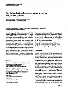
(2) Sensor network is a homogeneous network. In addition to the base station, the other nodes are considered to have equal status and initial energy. Here, it is worthy to notice that the energy of nodes cannot be added in the process of data gathering. (3) All nodes have some storage space and certain capability of data fusion and can take turns to be cluster heads. The system structure of the proposed RCCSDG method is depicted in Figure 2. In first phase, suppose that the 𝑊 nodes of whole networks would form 𝐼 clusters according to the clustering mechanisms, each cluster including one CH and (𝑁𝑖 − 1) noncluster head (non-CH) nodes. It should be noted here that 𝑁𝑖 is the number of nodes in cluster i. Let CH𝑖 denote the cluster head of cluster i and 𝑑𝑖 represent the sensor readings obtained by the 𝑖th node in cluster i. In transmit phase, all non-CH nodes transmit their readings to that corresponding cluster head CH𝑖 directly. Once these readings are received, the cluster head CH𝑖 gets 𝑁𝑖 readings which can be denoted as di = [𝑑1 , 𝑑2 , . . . , 𝑑𝑁𝑖 ], including 𝑁𝑖 − 1 readings from non-CH nodes and one reading from its own. Then, the raw readings [𝑑1 , 𝑑2 , . . . , 𝑑𝑁𝑖 ] are converted into ascending 󸀠 ] at order and form a new sequence d󸀠i = [𝑑1󸀠 , 𝑑2󸀠 , . . . , 𝑑𝑁 𝑖

󸀠 . After that, CH𝑖 CH𝑖 , where 𝑑1󸀠 < 𝑑2󸀠 < ⋅ ⋅ ⋅ < 𝑑𝑁 𝑖 󸀠 multiplies the new sequence di by a random matrix Φi and then sends the product yi to the sink. Notice that yi = Φi d󸀠i has 𝑚𝑖 measurements. Similarly, each CH transmits their information to the sink similar to the process above. Finally, the sink receives y = ∪Ii=1 yi , the compression information of all clusters. And the sum of the measurements sent to the sink is ∑I𝑖=1 𝑚𝑖 = 𝑀. At the sink, the original data can be reconstructed from yi by using reconstruction algorithm. The ̂󸀠. reconstructed data of cluster i is denoted by d i Under such design mode, all intracluster non-CH nodes only transmit their readings to their CH, and each CH transmits 𝑚𝑖 information to the sink. If each cluster contains the same number of nodes 𝑁𝑖 = 𝑁 and sends 𝑚 information to the sink, the communication load of whole network is 𝐼 ∗ (𝑁 − 1) + 𝐼 ∗ 𝑚 = 𝑊 + 𝐼 ∗ (𝑚 − 1). Because of 𝑚 ≪ 𝑁, the communication load of the RCCSDG method is far less than 𝑊∗𝑚. Therefore, the RCCSDG method can further compress the data by using simple linear operation. In order to reduce the delay, an improved (TDMA) scheme is adopted in our data gathering scheme. To make the delay of data gathering as short as possible, we adopt an improved TDMA2 (timedivision multiplexing access) scheduling scheme which is composed of three phases. Within cluster, each sensor at

4 regular time intervals generates a field value and transports it to its CH according to the TDMA scheme. And the CH of cluster can gather the sensed data from the sensors of the cluster simultaneously. It is well known that CSDG is able to recover the raw sensed data with high probability from few measurements when the data are sparse or compressible in some certain domains such as DCT, infinite difference, or Wavelet. However, the sparsity of most sensed signals in real world is not perfect. In some actual situations, the sensed data of adjacent nodes are not very uniform or vary greatly although they are close to each other on the physical position. When the sensed signals are not smooth enough, the sparsity of the data is not straightforward and even not sparse enough in transformed domains. As an example, Figure 3(a) shows a 72-dimensional out-of-order signal which has a great deal of volatility and worse smoothness. Obviously, it is not sparse itself. Figures 3(b), 3(c), and 3(d) give the corresponding sparse representation in three transformed domains, respectively. We set a threshold ℎ = 0.5; if the value of coefficients is lower than ℎ, they will be set as zero. Then the sparsity of signal is 57, 60, and 51 in TV, DCT, and DWT, respectively. Hence, the sparsity of the signal is also very poor in transformed domains. In this case, using current CS methods for data gathering usually cannot achieve good performance. As we know, the number of required measurements for reconstruction is in direct proportion to the sparsity of the signal. To guarantee the accuracy of data recovery, it needs to transmit more measurements in such situations. Therefore, if we can find a proper representation basis Ψ that obtains the sparsest representation or improves the sparsity by some simple preprocessing, it can effectively reduce the number of measurements using CS. Excitingly, we find that the signals are very smooth and have sparsest representation in TV domain when sorted into ascending order by their amplitudes; the results are shown in Figure 4. Figure 4(a) is the results by sorting the same original data of Figure 3(a) into ascending order; Figure 4(b) plots the sparse coefficients of this new signal in TV domain. One can see that most sparse coefficients are close to zero and only 5 values are relatively large; thus its sparsity is approximately 5. To check whether the other sensor data after reshuffling also have good sparsity, we compute the sparsity of light data, humidity data, and voltage data in different domains. In our tests, every type of sensor has 60 groups and every group contains 72 data items. We compute the sparsity of every group and the average sparsity of all groups as a result. The statistical results are presented in Table 1. We found that the sparsity of sensor data after reshuffling is always lower than the TV, DCT, and DWT in all the scenarios under investigation. These results indicate that the sensor data after sorting have a good sparsity in TV domain. Motivated by this investigation, we can improve the sparsity of the data signal through the use of a simple pretreatment on the raw sensed data. When the CH receives the raw sensed data d, which are sorted into ascending order through a simple preprocessing (namely, reshuffling operation) by CH firstly, then the result after preprocessing will be compressed by linear compressed

International Journal of Distributed Sensor Networks Table 1: Statistical average sparsity of sensor data in different domains.

TV DCT DWT Reshuffling + TV

Light data

Humidity data

Voltage data

23.5833 69.2167

68.03 67.85

68.383 68.83

46 8.13

66.93 22.9167

71.95 24.05

projection and the compression information will be transmitted to the sink. Through the reshuffling operation and linear compressed projection, each cluster can effectively reduce the communication cost. And such process is reasonable because the CH has a certain ability of data processing and the additional computing power is so small that it can be ignored. For the monitoring applications, the change of sensed data usually varies slowly within short time intervals. In other words, the sensed data have excellent temporal stability in a short time. So, in this short period, it can be assumed that the sparsity of this signal will not change and the sensed data can be arranged in the same order. Utilizing this feature, we just reorder data periodically according to empirical knowledge, which can further reduce energy consumption of the network.

3. Reshuffling Clustering Compressed Sensing Based Data Gathering Method In this section, we will describe the details of our proposed RCCSDG scheme and its implementation. It consists of three parts: (1) sensing part, (2) data compressed on CH, and (3) data recovery. 3.1. Sensing Part. As we know, the cluster route is capable of supporting the large-scale WSNs. In this subsection, we choose the LEACH to solve the problem of limited network scale of planar route. Here, the LEACH is a self-adaptive clustering algorithm whose execution process is cyclical, and each cycle is divided into two stages, namely, the establishment of cluster and data communication. (1) According to LEACH, the whole network is divided into 𝐼 clusters and each cluster has one cluster head. The non-CH nodes will independently join the corresponding cluster according to distance and then send the joined message to the CH. (2) When the cluster is set up, all non-CH nodes send the readings to their own CH. And the non-CH nodes only communicate with their own CH directly. The topology of cluster is useful to the application of distributed algorithms, because it is suitable for the largescale network. In addition, the clustering algorithm that uses periodic selection of cluster head can effectively balance the network energy consumption and prolong the lifetime of the network.

International Journal of Distributed Sensor Networks 20 13 7

0

10

20

30

40

50

60

5

70

8 0 −8

0

10

(a) Original signal

8 0 −8

0

10

20

30

40

20

30

40

50

60

70

60

70

60

70

(b) Representation in TV domain

50

60

70

8 0 −8

0

10

(c) Representation in DCT domain

20

30

40

50

(d) Representation in DWT domain

Figure 3: An out-of-order signal in transformed domains. 20

8

10

0

0

−8

0

10

20

30

40

50

60

70

(a) Sensor readings sorted into ascending order

0

10

20

30

40

50

(b) Representation in TV domain

Figure 4: An ascending order signal in TV domain.

3.2. Data Compression on CH. Due to all the sensed data in the cluster being collected by the CH, these received signals can be compressed by the CH using CS theory. The premise of CS theory is that the signal is 𝐾-sparse in a certain domain, and the amount of measurements 𝑀 is proportional to sparsity 𝐾. CS can turn an 𝑁-dimensional signal into 𝑀-dimensional (𝑀 ≪ 𝑁) while still keeping the information capacity. If we need to decrease the amount of data transmission, the sparsity 𝐾 of sensor readings should be reduced. However, how to exploit the sparsity of sensor readings is not straightforward in actual situation. It is well known that the smoother the sensed data is, the sparser those signals will be, and it is the most sparsest when the sensed data are sorted into ascending order. In light of this investigation, we proposed a new compressed sensing data aggregation algorithm based on reshuffling, which can decrease the data transmission of the cluster. And this data aggregation algorithm consists of two parts. The first is the reshuffling algorithm that aims to improve the sparsity. And the second is the linear compressed projection which can reduce the amount of data sampling by using compressed sensing technology. 3.2.1. Reshuffling Algorithm. Assume that di = [𝑑1 , 𝑑2 , . . . , 𝑑𝑁𝑖 ]𝑇 is the original sensors data sequence received by the CH, where 𝑑𝑖 denotes the reading of node 𝑖. We set 𝑑𝑗 representing the 𝑗th element of sequence d and compare all adjacent data from 1 to 𝑁𝑖 in turn, such as 𝑑𝑗 and 𝑑𝑗+1 . If 𝑑𝑗 > 𝑑𝑗+1 , exchange the elements in the 𝑗th and (𝑗 + 1)th position; then compare with the next data in the same way. Otherwise, keep the data unchanged in the 𝑗th and the (𝑗 + 1)th position, and directly compare with the data in next position. It will generate a new sequence d󸀠i when the comparison is finished, and then repeat the previous operations for every new d󸀠i until the elements of data are in an ascending sort order 𝑑1󸀠 < 𝑑2󸀠 < 󸀠 󸀠 ⋅ ⋅ ⋅ < 𝑑𝑁 < 𝑑𝑁 . The elements of initial data can be sorted 𝑖 −1 𝑖 into ascending order through such operations as that shown

in Algorithm 1. And the new data vector can be represented by 𝑍 ↑ (di ) , d󸀠i = 𝐴

(1)

𝑍 where 𝐴 ↑(a) is the reshuffling operation for sorting the elements of vector a in ascending order. It is easy to show that the algorithm needs 𝑁𝑖 ∗ (𝑁𝑖 − 1)/2 comparisons and 𝑁𝑖 ∗ (𝑁𝑖 − 1)/2 shift operations to transfer di into d󸀠i for the worst-case scenario when the original data sequence is in a reverse order.

3.2.2. Linear Compressed Projection. Compressing the signals of sensors is the principal aim of data aggregation for WSNs. Each CH of the network utilizes the linear compressed projection to realize data compression. After getting the reshuffling preprocessing data d󸀠i , each CH synchronously generates a Gaussian random matrix Φi , and then the CH multiplies the Gaussian random matrix Φi by the data vector d󸀠i to produce the projection yi , where d󸀠i is an ascending sequence. By the linear compressed projection, the dimensions of the data are reduced to 𝑀 (𝑀 ≪ 𝑁) dimensions from 𝑁 dimensions. Thereby it can decrease the communication overhead. Linear compressed projection model for whole network can be represented as y1 y2

(.)=( .. yI ⏟⏟⏟⏟⏟⏟⏟⏟⏟⏟⏟⏟⏟⏟⏟⏟⏟ y:𝑀×1

d󸀠1

Φ1

d󸀠2

Φ2 d

)( . ) . ..

(2)

ΦI ⏟⏟⏟⏟⏟⏟⏟⏟⏟⏟⏟⏟⏟⏟⏟⏟⏟⏟⏟⏟⏟⏟⏟⏟⏟⏟⏟⏟⏟⏟⏟⏟⏟⏟⏟⏟⏟⏟⏟⏟⏟ d󸀠I ) ⏟⏟⏟⏟⏟⏟⏟⏟⏟⏟⏟⏟⏟⏟⏟⏟⏟ ( Φ:𝑀×𝑊 d󸀠 :𝑊×1

Through the data aggregation, each CH just needs to transmit the measurement vector yi , but not all sensor data, to the sink. It can be concluded from (2) that the compression

6


collect the intra-cluster readings di = [𝑑1 , 𝑑2 , . . . , 𝑑𝑁𝑖 ]𝑇 for 𝐾 = 1 to end do (𝐾 is the comparison round) for 𝑗 = 1, 𝑗 ∈ (1, 𝑁𝑖 ) do compare the data on the adjacent location 𝑑𝑗 , 𝑑𝑗+1 if 𝑑𝑗 ≤ 𝑑𝑗+1 then exchange the elements of 𝑗th and (𝑗 + 1)th. else keep the data in 𝑗th and (𝑗 + 1)th position. end if end for end for 󸀠 𝑇 ] output ascending sequence d󸀠i = [𝑑1󸀠 , 𝑑2󸀠 , . . . , 𝑑𝑁 𝑖 Algorithm 1: Reshuffling data into ascending order.

for i = 1 to 𝐼 do collect the intra-cluster readings di (𝑡0 ) = [𝑑1 , 𝑑2 , . . . , 𝑑𝑁𝑖 ]𝑇 at t 0 . for 𝑡 = 𝑡0 to end do if (𝑡 − 𝑡0 ) %𝑇 = 0 󸀠 𝑇 using Reshuffling Algorithm get sequence d󸀠i (𝑡) = [𝑑1󸀠 , 𝑑2󸀠 , . . . , 𝑑𝑁 ] 𝑖 else collect readings according to the data structure of d󸀠i (𝑡 − Δ𝑡) as di (𝑡). end if linear projection yi (𝑡) = Φi di (𝑡) or Φi d󸀠i (𝑡) then transmit yi (𝑡) to the sink. end for end for Algorithm 2: Linear compressed projection.

information y has 𝑀 measurements, far less than the number of original data 𝑊. Beyond that, data sorted into ascending order through reshuffling algorithm can effectively reduce the data sparseness and thus decrease the total number of measurements to 𝑀. And using this way in data compression, we can reconstruct the raw data of all nodes in the sink through numerical methods. Since many sensed signals such as temperature and humidity have excellent temporal stability in a short time and the data sorted into ascending order is more sparse than the original order, as a result, the sensed data collected at next interval can also be considered to be sparse when organized in the same order. But as we know, with the monitoring time growing, the signals will change and the sparsity of them may degrade. When sparsity is poor, more measurements will be needed for accurate reconstruction; otherwise the reconstruction will fail. Meanwhile, reordering the elements of data signal every time to obtain optimal measurements for exact reconstruction will increase extra complexity and energy consumption. To cope with this situation, we update the ordering periodically. We set an updated cycle 𝑇 according to the prior knowledge firstly. During the updated cycle 𝑇, the sensed data will be reshuffled just one time and keep the order. When the time interval between the current acquisition and first order is integer times of 𝑇, the CH will update the ordering of di (𝑡) and use

the new arrangement for data compression in the following 𝑇. The main process is shown in Algorithm 2. 3.3. Data Recovery. CS theory points out that when the number of measurements 𝑀 satisfies (3), a 𝐾-sparse signal may be exactly reconstructed: 𝑀 ≥ 𝑐 ⋅ 𝐾 ⋅ log (

𝑁 ), 𝐾

(3)

where 𝑐 is a positive constant and 𝑁 is the length of signal here. Equation (3) also indicates that the smaller the 𝐾 is, the fewer the measurements are needed for accurate reconstruction. In practice, 𝑀 = 3K∼4K can usually satisfy the condition of (3). The sink gathers all measurements y from every CH ̂󸀠 and takes a responsibility for recovering the sensor data d from these measurements. Because the measurements yi are obtained by linear compressed projection on the sensors data, it contains enough information for exact reconstruction, since the compression information y is an 𝑀-dimensional vector and the sensor data sequence d󸀠 is an 𝑁-dimensional vector, and 𝑀 ≪ 𝑁. Thus, (2) is an underdetermined equation and cannot recover the original signal directly. We have investigated in this paper that the sensors data after reshuffling have a better sparsity in TV domain. Putting this


7

Input: observation matrix Φ, sparse matrix Ψ, observation vector 𝑦, the number of iterations 𝐾, terminating condition 𝛿; Output: sparse coefficients 𝑥 ̃ 0 = 𝑦, 𝛾𝑛 = 𝛼𝑛 (𝑛 = 1, . . . , 𝑁), 𝑑𝑛 = 1 (𝑛 = 1, . . . , 𝑁), Initially set: 𝑘 = 1, set of indexes Λ 0 = ⌀, 𝑅 ̃ 1 ‖2 = ‖𝑅 ̃ 0 ‖2 − |𝑥1 |2 , set of indexes Λ 1 = Λ 0 ∪ {𝑙1 }. 𝑙1 = arg max | > |, 𝜓1 = 𝛼𝑙1 = 𝛽1 , 𝑥1 = ⟨𝛼𝑙1 , 𝑦⟩, ‖𝑅 Looping execution steps: Step 1. for 𝑛 = 1, . . . , 𝑁, compute: 𝛾𝑛 = 𝛾𝑛 − 𝜓𝑘 ⟨𝜓𝑘 , 𝛼𝑛 ⟩, 𝑏𝑛 = ⟨𝛾𝑛 , 𝑦⟩, 𝑑𝑛 = 𝑑𝑛 − |⟨𝜓𝑘 , 𝛼𝑛 ⟩|2 (or 𝑑𝑛 = ‖𝛾𝑛 ‖2 ) if |𝑏𝑛 | < 𝜀, 𝑒𝑛 = 0, otherwise 𝑒𝑛 = |𝑏𝑛 |2 /𝑑𝑛 . Step 2. 𝑘 = 𝑘 + 1, set 𝑙𝑘 = arg max 𝑒𝑛 , ̃ 𝑘 ‖2 = ‖𝑅 ̃ 𝑘−1 ‖ − 𝑒𝑙𝑘 , update Λ 𝑘 = Λ 𝑘−1 ∪ 𝑙𝑘 , ‖𝑅 assign 𝜓𝑘 = 𝛾𝑙𝑘 /√𝑑𝑙𝑘 , 𝛽𝑘 = 𝛾𝑙𝑘 /𝑑𝑙𝑘 , compute 𝑥𝑘 = ⟨𝛽𝑘 , 𝑦⟩. Step 3. for 𝑛 = 1, . . . , 𝑘 − 1, compute: 𝛽𝑛 = 𝛽𝑛 − 𝛽𝑘 ⟨𝛼𝑙𝑘 , 𝛽𝑛 ⟩, 𝑥𝑛 = 𝑥𝑛 − ⟨𝛽𝑛 , 𝑥𝑙𝑘 ⟩𝑥𝑘 . ̃ 𝑘 ‖2 ≤ 𝛿. Step 4. repeat Step 1, Step 2, Step 3, until 𝑘 > 𝐾, or ‖𝑅 Algorithm 3: OOMP algorithm.

prior knowledge into the signal model, the sink can reconstruct the raw sensed data via solving the 𝑙0 -minimization problem [23, 24]: min s.t.

‖x‖𝑙0 y = Φd󸀠 = ΦΨ−1 x = Φ󸀠 x,

(4)

where Ψ is the sparse matrix and x is the sparse coefficients. Solving 𝑙0 -minimization problem can achieve precise reconstruction, but it is a NP problem. The Optimized Orthogonal Matching Pursuit (OOMP) [25] approach improved on the basis of the Matching Pursuit (MP) [26] and Orthogonal Matching Pursuit (OMP) [27] has a good convergence and high reconstruction accuracy. Given this, we choose OOMP algorithm to reconstruct the compressed data and the algorithm is summarized asin Algorithm 3, where 𝛼𝑛 is the ̃ 𝑘 is the 𝑘th order residue, and 𝑙𝑘 is the index dictionary atom, 𝑅 ̃ 𝑘 ⟩| takes the maximal value, where ⟨⋅, ⋅⟩ for 𝛼𝑙𝑘 when |⟨𝛼𝑛 , 𝑅 represents the inner product.

4. Energy Consumption and Delay Analysis of RCCSDG Method 4.1. Energy Consumption Analysis of RCCSDG. The previous section has described how to collect and recover the sensed data in RCCSDG scheme, and this section will investigate the energy consumption of RCCSDG. In the process of data gathering, non-CH nodes transmit their sensed data to the CH that they belong to, and the CH is responsible for aggregating the data and sending the results to the sink. Since the CH nodes are the main contribution to energy consumption in WSNs, thus here we only analyze the energy consumption of the CH. The total energy consumption of the CH is comprised of two main components: data processing energy consumption-𝐸DP and data transmission energy consumption-𝐸TR .

Therefore, the energy consumption of the CH can be formed as 𝐸CH = (𝐸DP + 𝐸TR ) .

(5)

For simplicity, we only consider the situation of one cluster in the following analysis. 4.1.1. Analysis of 𝐸DP . The energy consumption of CPU is determined by the number of operations for signal processing. In other words, energy consumption of the data processing is scaled with the operation during the process of signal processing. In RCCSDG scheme that we proposed, all sensed data within cluster are sorted into ascending order through reshuffling algorithm first and then acquire 𝑚 measurements through linear compressed projections on CH. So the energy consumption of CH for data processing also includes reshuffling cost (𝐸DP-RS ) and data compression cost (𝐸DP-CS ) except that of data reading and writing. For reshuffling algorithm, it requires no more than 𝑁 ∗ (𝑁 − 1)/2 comparisons and 𝑁 ∗ (𝑁 − 1)/2 shift operations for the reverse order, as mentioned in Section 3. And the complexity of reshuffling algorithm is 𝑂(𝑁2 ). The 𝑚 random measurements are acquired through a linear compressed projection on 𝑁 sensor data. It is noted that the linear compressed projection is a matrix multiplication operation in essence. And matrix multiplication is the process of multiplying the 𝑚×𝑁 measurement matrix by an 𝑁-dimensional data vector to get an 𝑚-dimensional vector. It needs to execute 𝑚 ∗ 𝑁(𝑁 − 1) additions and 𝑚 ∗ 𝑁 multiplications. So the total energy consumption of cluster head for data processing can be expressed as a sum: 𝐸DP = 𝑁𝜉mrd +

𝑁 (𝑁 − 1) (𝜉cmp + 𝜉sft ) ⏟⏟⏟⏟⏟⏟⏟⏟⏟⏟⏟⏟⏟⏟⏟⏟⏟⏟⏟⏟⏟⏟⏟⏟⏟⏟⏟⏟⏟⏟⏟⏟⏟⏟⏟⏟⏟⏟⏟⏟⏟⏟⏟ 2 𝐸DP-RS

+ 𝑚𝑁𝜉 ⏟⏟⏟⏟⏟⏟⏟⏟⏟⏟⏟⏟⏟⏟⏟⏟⏟⏟⏟⏟⏟⏟⏟⏟⏟⏟⏟⏟⏟⏟⏟⏟⏟⏟⏟⏟⏟⏟⏟⏟⏟⏟⏟⏟⏟⏟⏟ add + 𝑚 (𝑁 − 1) 𝜉mul + 𝑚𝜉mwr , 𝐸DP-CS

(6)

8


where 𝜉mrd = 9.90 nJ, 𝜉cmp = 3.30 nJ, 𝜉sft = 3.30 nJ, 𝜉add = 3.30 nJ, 𝜉mul = 9.90 nJ, and 𝜉mwr = 9.90 nJ are the energy consumption values for memory reading, comparison, shift operation, addition operation, multiplication, and memory writing in CPU of sensor node [28]. If the cluster head refreshes the ordering of data every 𝑇, the computation energy can be further reduced (reduce (𝑇 − 1) ∗ 𝐸DP-RS ) and represented by 𝐸DP (𝑇) =

𝑁 (𝑁 − 1) (𝜉cmp + 𝜉sft ) 2

(7)

+ 𝑇 (𝑁𝜉mrd + 𝑚𝑁𝜉add + 𝑚 (𝑁 − 1) 𝜉mul + 𝑚𝜉mwr ) . 4.1.2. Analysis of 𝐸𝑇𝑅 . In the process of data communication, the CH receives the sensed data from all non-CH nodes and transmits the compression information to the sink. Thus the energy consumption of 𝐸TR includes sending message (𝐸TR-SD ) and receiving message (𝐸TR-RE ). Here, we adopt wireless transmission energy consumption model proposed in [21] for analysis of 𝐸TR . Depending on distance between the transmitter and the receiver, free space model and the multipath fading model are utilized, respectively. When the transmission distance 𝑑 is less than the threshold 𝑑0 , we choose the free space model. Otherwise, the multipath fading model is adopted. To send 𝑙-bit data for a distance of 𝑑, the energy consumption model of wireless transmission can be presented as follows: 2 {𝑙 ∗ 𝐸elec + 𝑙 ∗ 𝜀fs ∗ 𝑑 , 𝑑 ≤ 𝑑0 𝐸TR-SD = { 𝑙 ∗ 𝐸elec + 𝑙 ∗ 𝜀mp ∗ 𝑑4 , 𝑑 > 𝑑0 . {

(8)

Also, in order to receive 𝑙-bit data, the sensor expends 𝐸TR-RE = 𝑙 ∗ 𝐸elec ,

(9)

where 𝐸elec is the energy consumption of transmission circuit to send or receive 1-bit data. The 𝜀fs and 𝜀mp are represented as the power consumption of the launch amplifier to transmit 1-bit data in different model. In RCCSDG scheme, we assume that there are 𝑁 nodes in cluster (one CH node and (𝑁 − 1) non-CH nodes) and the size of each data packet is 𝐿 bytes. The CH receives (𝑁 − 1) ∗ 𝐿-byte data from all nonCH nodes within cluster and sends 𝑚-byte measurements to the sink. According to (8) and (9), the transmission energy consumption of CH in each data gathering cycle can be formulated as 𝐸TR = 𝐸TR-RE + 𝐸TR-SD 2 {8𝐿 ∗ ((𝑁 − 1) 𝐸elec + 𝑚𝐸elec + 𝑚𝜀fs 𝑑 ) , 𝑑 ≤ 𝑑0 (10) ={ 8𝐿 ∗ ((𝑁 − 1) 𝐸elec + 𝑚𝐸elec + 𝑚𝜀mp 𝑑4 ) , 𝑑 > 𝑑0 . {

From (10), we can conclude that the energy consumption for transmission, 𝐸TR , only depends on the number of measurements 𝑚 when the distance 𝑑 and the size of cluster 𝑁 are fixed. We have proved that the RCCSDG method can

improve the sparsity of data by a simple pretreatment on original data and greatly reduce the number of measurements. Therefore, although the RCCSDG scheme increases some extra computation, the energy consumption of data transmission can be greatly reduced. In the next section, we will verify the theory analysis of energy consumption of CH by simulation. 4.2. Delay Analysis of RCCSDG. In this section, we analyze the delay of RCCSDG. The analysis can be done in a way similar to [29]. Recall that the proposed model implements two-hop WSNs based on TDMA2 scheduling scheme. In this scheme, each node within the same cluster sends data to cluster by TDMA-1 and the cluster headers compress the signals and transmit the random projections to sink by TDMA-2. The processing schedule in one round is shown in Figure 5. To make the delay of data gathering as short as possible, we adopt a pipeline TDMA2 scheduling scheme composed of three phases. First Phase. The sink finds cluster 𝐶𝑚 containing the maximum number of nodes and the cluster head can firstly forward the random compressed data to sink. Second Phase. Each node of cluster sends the data to the cluster head by TDMA scheduling method. After receiving the data of all nodes in this cluster, the cluster head compresses these data by random projection and the cluster head of 𝐶𝑚 firstly forwards their compressed information to the sink. Third Phase. After the cluster head of the 𝐶𝑚 forwards their compressed information to the sink. Other cluster heads forward their randomly compressed information to the sink by TDMA2 scheduling method. Definition 1. The delay of data gathering 𝐷 is the time when the last random measurement reaches the sink. The delay of RCCSDG based on pipeline TDMA2 scheduling scheme is 𝑚

𝐼

𝑖=1

𝑖=1

𝐷 = ∑ 𝑇𝐶𝑚 ∗𝑖 + 𝑇DP∗𝑚 + ∑ 𝑇Ch∗𝑖 ,

(11)

where 𝑇𝐶∗𝑖 is the 𝑖 node time slot of cluster 𝐶𝑚 , 𝑇DP∗𝑚 is processing time of cluster 𝐶𝑚 including reshuffling time and compressing time, and 𝑇Ch∗𝑖 is forwarding time of cluster 𝐶𝑖 . Let 𝑡sen be the time of sending one bit and 𝑡proc is the time of processing one bit. Assume that the compressing ratio is 𝑐 ratio and equal to all clusters. If we choose the quick sort method as reshuffling algorithm, its worst-case performance is 𝑂(𝑁2 ), while this is rare. In practice choosing a random pivot almost certainly yields 𝑂(𝑁 ∗ log 𝑁) performance, and the complexity of reshuffling algorithm is 𝑂(𝑁∗log 𝑁). Based on these conditions, (11) can be rewritten as 𝐷 = 𝑁𝑚 ∗ 𝑡sen + 𝑂 (𝑁𝑚 ∗ log 𝑁𝑚 ) ∗ 𝑡proc + 𝑐 ratio ∗ 𝑁 ∗ 𝑡sen = (𝑁𝑚 + 𝑀) ∗ 𝑡sen + 𝑂 (𝑁𝑚 ∗ log 𝑁𝑚 ) ∗ 𝑡proc .

(12)


9

TDMA-1 TC(𝐼−1) ∗1

TC(𝐼−1) ∗2

···

TDMA-2 TC(𝐼−1) ∗N(𝐼−1)

TCh∗(I−1)

TDP∗(I−1) ···

.. . TC1 ∗1

TC1 ∗2

···

TC1 ∗N1

TDP∗1

TC𝑚 ∗1

TC𝑚 ∗2

···

TC𝑚 ∗N𝑚

TDP∗m

TCh∗1 TCh∗m

Time slot 2

Figure 5: The pipeline TDMA scheduling scheme.

Table 2: Simulation parameters. Parameter Radio dissipation (𝐸elec ) Distance threshold (𝑑0 ) Data packet size (𝐿) 𝜀f h 𝜀mp Size of cluster (𝑁)

Default value 50 nJ/bit 80 m 128 bytes 100 pJ/bit/m2 0.015 pJ/bit/m4 200

From (12), we can conclude that the worst delay case is partitioned to one cluster only and the best delay case is divided into 𝐼 uniform clusters. So the delay 𝐷 of RCCSDG is (𝑁 + 𝑀) ∗ 𝑡sen + 𝑂 (𝑁 ∗ log 𝑁) ∗ 𝑡proc ≤ 𝐷 ≤(

𝑂 (𝑁 ∗ log 𝑁) 𝑁 + 𝑀) ∗ 𝑡sen + ( ) ∗ 𝑡proc . 𝐼 𝐼

(13)

5. Simulation Results In the following subsection, we first verify the efficiency of the RCCSDG scheme by energy consumption simulation and then evaluate reconstruction accuracy over real sensed data. The numerical results show that the RCCSDG method is effective in reducing energy consumption in deed. Furthermore, the reconstruction results also demonstrate the better performance of the RCCSDG method. 5.1. Energy Consumption Simulation. The RCCSDG method can effectively reduce the energy consumption by sacrificing a small amount of computing resource. And during the data gathering, the CH, which plays an important role in data processing and data transmission, is the main aspect of network energy consumption. In this subsection, we will give the simulation results of CH energy consumption and verify the efficiency of the RCCSDG method. Table 2 lists the main parameters used in the simulations. To reduce the energy consumption of CH, we need to know the factors which influence the energy consumption of CH. Here, we have conducted a numerical analysis to the

factors that may influence energy consumption of the CH in terms of data transmission and data processing, and the results are shown in Figure 6. From (10), it indicates that the energy consumption of data transmission is determined by the transmission distance and the number of measurements when the size of cluster is fixed. And this is also shown in Figure 6(a). The energy consumption of data transmission is proportional to the amount of measurements when the distance is constant. And the closer the distance between node and CH is, the faster the energy is consumed. In particular, when the distance is greater than threshold 𝑑0 (here 𝑑0 = 80 m), the energy consumption will quicken significantly. Differently from transmission cost, the energy consumption of data processing is only determined by the number of measurements and the size of cluster. As shown in Figure 6(b), it is easy to note that the energy consumption of CH computation increases with the increase of the cluster size and measurements. Therefore, we can conclude that more energy can be saved with further decreasing the measurements when the distance and the size of cluster are fixed. Luckily, the RCCSDG scheme can recover the data signals with fewer measurements. By using a pretreatment on original data at CH, the RCCSDG we proposed can decrease the measurements to be transmitted, but it introduces some computation cost. To validate the validity of this scheme, we need to demonstrate that the added computation is far smaller than the reduced transmission. For this, we plot in Figure 7 the energy consumption of transmission and computation of RCCSDG and conventional CS scheme when we set 𝑑 = 80, 𝑁 = 200. The black line is the transmission cost, the red line depicts the computation consumption of RCCSDG, and the pink line represents the computation energy consumption of conventional CS scheme. Obviously, as the compression ratio grows, both transmission cost and computation cost increase, and the transmission cost is always far larger than computation cost. Here, compression ratio is defined as the ratio of the number of measurements to the number of original data. The RCCSDG method can yield the same results as the conventional CS scheme with a lower compression ratio, which will be validated in next subsection. During our experiments, we suppose that RCCSDG has the same performance at ratio = 0.1 while the ratio of conventional

10

International Journal of Distributed Sensor Networks ×105 7 Energy consumption of computation (/nJ)

Energy consumption of transmission (/nJ)

×107 15

10

5

6 5 4 3 2 1

0 100

80

60 40 Dist 20 ance (/m)

0

0

100 80 60 40 ts 20 suremen r of mea Numbe

0 200

150 100 50 Size o f clus ter

(a)

0

0

200 150 100 ts 50 suremen r of mea Numbe

(b)

Figure 6: Transmission energy consumption and computation energy consumption of CH.

×108

Energy consumption (nJ)

1.5

1.0 0.5

E1

0.004 0.002

E2

0.0 0.0

0.2

0.4 0.6 Compression ratio

0.8

Transmission power consumption Computation for RCCSDG Average computation for RCCSDG every T Computation for conventional CS

Figure 7: Energy consumption of RCCSDG and conventional CS scheme.

CS scheme is 0.5. Compared to conventional CS scheme, the reduced transmission consumption and the added computation cost of the RCCSDG method are expressed as 𝐸1 and 𝐸2 (the difference between red line and pink line), respectively, as marked in Figure 7. It is clear that 𝐸1 (5.652 ∗ 107 nJ) is far larger than 𝐸2 (1.313 ∗ 105 nJ), which make it evident that the added computation cost is far smaller than the reduced transmission consumption in RCCSDG scheme. Therefore, the RCCSDG method can significantly decrease the energy consumption of CH eventually and is superior to conventional CS scheme. Since most signals have excellent temporal stability in a short time, the ordering of data is refreshed periodically. Note that ordering process takes place at CH and only

affects the energy consumption of computation. The blue line in Figure 7 represents the average computation dissipation when refreshing the ordering every 𝑇 (here 𝑇 = 10). Through refreshing the order periodically, the computation consumption of RCCSDG goes down from the red line to the blue line in Figure 7. The blue line is close to the pink line, and the difference between RCCSDG and conventional CS method will decrease as the 𝑇 increases. Thus it can indicate that updating the ordering of data in a stable period can further reduce the computational burden. The results of simulation above show that the energy consumption of CH is mainly contributed to the data transmission, and the energy consumption for signal processing is so small that it can be neglected. So the RCCSDG method can be used to reduce the energy consumption although it increases a little computational complexity. 5.2. Reconstruction Performance Simulation. In order to verify the reconstruction performance of the RCCSDG method we proposed, we use the following two evaluation criterions (RMSE and PSNR) in this paper. Formally, the RMSE (rootmean-square error) is defined as (14), and the PSNR (peak signal-to-noise ratio) is defined as (15): RMSE = √

1 𝑁 ̂ 2, ∑ (𝑑 − 𝑑) 𝑁 𝑖=1 𝑖

PSNR = 10 ∗ log10 (

2 𝑑pp

RMSE

(14)

),

(15)

where 𝑁 is the length of the data signal, 𝑑𝑖 is the original sensor data of node 𝑖, 𝑑̂ represents the reconstructed value of the 𝑖th node, and 𝑑pp represents the peak-to-peak value of signal. In our paper, we carry out simulation on real sensed datasets. The datasets contain 2666 humidity readings from 31 sensor nodes and they are collected by the Department of


11

20

RMSE

15

10

5

0 0.1

0.2

0.3

0.4

0.5

0.6

0.7

0.8

Dumping ratio (1 − sampling ratio)

RCCSDG CSDG-OOMP CSDG-TV

Figure 8: Comparing reconstruction RMSE of RCCSDG, CSDGOOMP, and CSDG-TV at moment 𝑡0 . 42 40 Reconstruction PSNR

38 36 34 X: 0.7 Y: 30.49

32 30 28 26 24 22 20 0.1

0.2

0.3

0.4 0.5 Sampling ratio

0.6

0.7

0.8


Figure 9: Comparing reconstruction PSNR of RCCSDG, CSDGOOMP, and CSDG-TV at moment 𝑡0 .

Information Engineering (DEI) of the University of Padova on March 24th, 2009. According to CS theory, the original data can be recovered at the sink by some algorithms. Firstly, we compare the recovery performance of RCCSDG with other data collection schemes at moment 𝑡0 . Figure 8 shows the reconstruction RMSE of RCCSDG, CSDG-OOMP, and CSDG-TV under different dumping ratio and Figure 9 gives the results of PSNR under different sampling ratio. Paper [19] points out that sampling rate is inversely linked to the packet loss rate. This means that the low sampling rate of sensor data is equivalent to the case of high packet loss rate. In this paper, the dumping ratio is defined as (1 − sampling ratio). In order to avoid fluctuation, the reconstructions are repeated 100 times. From the results of Figure 8, we can see that the RMSE of RCCSDG is the lowest one. Figure 9 apparently indicates that the recovery

performance by the three schemes increases as the sampling ratio 𝑟 increases. Nevertheless, the growth rate of PSNR by the RCCSDG scheme is faster than the other two schemes and the value is always larger than them at the same ratio. For example, the RCCSDG method outperforms conventional CS scheme reconstruction by up to about 9 dB at ratio 𝑟 = 0.4 in PSNR. And given the target PSNR, the ratio of RCCDG is lower than the other two schemes. For instance, to get the same PSNR = 30.49, the ratios of RCCDG, CSDG-OOMP, and CSDG-TV are 0.1, 0.7, and 0.8, respectively. The reason is that the sensor readings after reshuffling become piecewise smooth and more sparse. This means that, to achieve the same effect of reconstruction, the number of measurements required by the RCCSDG method is far less than CSDGOOMP and CSDG-TV scheme. In other words, the RCCSDG method can achieve better recovery performance under a lower compression ratio. Since the humidity data are not varied much in a short time and smooth when collected in the same order at next collecting moment, as shown in Figure 10, the sparsity of data can be regarded as not changed at this moment when data are arranged in the same order. But as monitoring time increases, the smoothness of the data will become worse, thus impacting the precision of data reconstruction. To handle this problem, the RCCSDG method rearranges the data ordering periodically based on the a priori knowledge. During this period, sensor data are reshuffled just one time and keep the order. By reordering data periodically, the RCCSDG method can make the sparsity of data always stay in a proper range, which can ensure achievement of accurate reconstruction with a small number of measurements. This is depicted by the simulation results in Figure 11. It shows the PSNR of data recovery with compression ratio 𝑟 = 0.4 and the reordered period 𝑇 = 20. From the results we can see that the average reconstruction PSNR is 34 and far better than the conventional CS scheme without ordering. Therefore, the RCCSDG method can effectively reduce the amount of data transmission and guarantee the reconstruction accuracy at the same time.

6. Conclusion This paper describes an energy-efficient data gathering scheme for WSNs by reshuffling cluster compressed sensing as described. We have found that the sensed data arranged into ascending order have better sparsity. Based on this principle, the cluster heads just adopt a simple preprocessing on original data to reshuffle the data into ascending order, which can greatly improve the sparsity and effectively minimize the amount of data transmission. We have investigated that the additional computation for preprocessing is small enough to be neglected. Besides, most sensor signals have excellent temporal stability in WSNs; we only update the ascending order of data periodically. By incorporating the temporal correlation, the energy consumption can be further reduced while guaranteeing the data reconstruction accuracy. Also we have demonstrated the theoretical analysis of the energy consumption and delay in detail when adopting the RCCSDG scheme. The simulation results based on real sensor data that

12

International Journal of Distributed Sensor Networks 40 35 30 20

10

5

15

20

40 35 30 20

30

25

5

(a) Sensor readings at time 𝑡

50 40 30 20

10

15

20

25

30

(b) Sensor readings at time 𝑡 + 10

10

5

15

20

25

30

(c) Sensor readings at time 𝑡 + 20

Figure 10: Sensor readings first ordered at time 𝑡 and sensor readings at 𝑡 + 10 and 𝑡 + 20.

References

36 35 Reconstruction PSNR

34 33 32 31 30 29 28 27 26 25

0

10

20

30

40 50 60 Monitoring time

70

80


Figure 11: The comparison of reconstruction results in a period of time at ratio = 0.4.

validate the energy efficacy and reconstruction accuracy of the RCCSDG scheme have been proposed. Considering the fact that the sensor data also contains low-rank structure information, our future work will investigate matrix completion to further improve the reconstruction accuracy and reduce the computational complexity so as to conserve the energy and ulteriorly extend the lifetime of network.

Conflict of Interests The authors declare that there is no conflict of interests regarding the publication of this paper.

Acknowledgment The work was supported by the National Nature Science Foundation of China (no. 61162015 and no. 31101081) and the Science and Technology Supported Project of Jiangxi Provincial (no. 20151BBE50095).

[1] C. W. Chen and Y. Wang, “Chain-type wireless sensor network for monitoring long range infrastructures: architecture and protocols,” International Journal of Distributed Sensor Networks, vol. 4, no. 4, pp. 287–314, 2008. [2] C. Wang, H. Ma, Y. He, and S. Xiong, “Adaptive approximate data collection for wireless sensor networks,” IEEE Transactions on Parallel and Distributed Systems, vol. 23, no. 6, pp. 1004–1016, 2012. [3] P. Kasirajan, C. Larsen, and S. Jagannathan, “A new data aggregation scheme via adaptive compression for wireless sensor networks,” ACM Transactions on Sensor Networks, vol. 9, no. 1, article 5, 26 pages, 2012. [4] S. Madden, M. J. Franklin, J. M. Hellerstein, and W. Hong, “TAG: a tiny aggregation service for ad-hoc sensor networks,” ACM SIGOPS Operating Systems Review, vol. 36, pp. 131–146, 2002. [5] A. Ciancio, S. Pattem, A. Ortega, and B. Krishnamachari, “Energy-efficient data representation and routing for wireless sensor networks based on a distributed wavelet compression algorithm,” in Proceedings of the 5th International Conference on Information Processing in Sensor Networks, pp. 309–316, ACM, Nashville, Tenn, USA, 2006. [6] K. Yuen, B. Liang, and B. Li, “A distributed framework for correlated data gathering in sensor networks,” IEEE Transactions on Vehicular Technology, vol. 57, no. 1, pp. 578–593, 2008. [7] G. Hua and C. W. Chen, “Correlated data gathering in wireless sensor networks based on distributed source coding,” International Journal of Sensor Networks, vol. 4, no. 1-2, pp. 13–22, 2008. [8] D. L. Donoho, “Compressed sensing,” IEEE Transactions on Information Theory, vol. 52, no. 4, pp. 1289–1306, 2006. [9] E. J. Candès, J. Romberg, and T. Tao, “Robust uncertainty principles: exact signal reconstruction from highly incomplete frequency information,” IEEE Transactions on Information Theory, vol. 52, no. 2, pp. 489–509, 2006. [10] E. J. Candès and M. B. Wakin, “An introduction to compressive sampling,” IEEE Signal Processing Magazine, vol. 25, no. 2, pp. 21–30, 2008. [11] S. Lee, S. Pattem, M. Sathiamoorthy, B. Krishnamachari, and A. Ortega, “Spatially-localized compressed sensing and routing in multi-hop sensor networks,” in Geosensor Networks, pp. 11–20, Springer, Berlin, Germany, 2009. [12] L. Xiang, J. Luo, and C. Rosenberg, “Compressed data aggregation: energy-efficient and high-fidelity data collection,” IEEE/ACM Transactions on Networking, vol. 21, no. 6, pp. 1722– 1735, 2013.

International Journal of Distributed Sensor Networks [13] J. Wang, S. Tang, B. Yin, and X.-Y. Li, “Data gathering in wireless sensor networks through intelligent compressive sensing,” in Proceedings of the IEEE Conference on Computer Communications (INFOCOM ’12), pp. 603–611, Orlando, Fla, USA, March 2012. [14] M. T. Nguyen and K. A. Teague, “Tree-based energy-efficient data gathering in wireless sensor networks deploying compressive sensing,” in Proceedings of the 23rd Wireless and Optical Communication Conference (WOCC ’14), pp. 1–6, IEEE, Newark, NJ, USA, May 2014. [15] W. Wang, M. Garofalakis, and K. Ramchandran, “Distributed sparse random projections for refinable approximation,” in Proceedings of the 6th International Conference on Information Processing in Sensor Networks (IPSN ’07), pp. 331–339, ACM, Cambridge, Mass, USA, April 2007. [16] C. Luo, F. Wu, J. Sun, and C. W. Chen, “Compressive data gathering for large-scale wireless sensor networks,” in Proceedings of the 15th Annual ACM International Conference on Mobile Computing and Networking (MobiCom ’09), pp. 145–156, ACM, Beijing, China, September 2009. [17] C. Luo, F. Wu, J. Sun, and C. W. Chen, “Efficient measurement generation and pervasive sparsity for compressive data gathering,” IEEE Transactions on Wireless Communications, vol. 9, no. 12, pp. 3728–3738, 2010. [18] J. Cheng, H. Jiang, X. Ma et al., “Efficient data collection with sampling in WSNs: making use of matrix completion techniques,” in Proceedings of the 53rd IEEE Global Communications Conference (GLOBECOM ’10), pp. 1–5, IEEE, Miami, Fla, USA, December 2010. [19] J. Cheng, Q. Ye, H. Jiang, D. Wang, and C. Wang, “STCDG: an efficient data gathering algorithm based on matrix completion for wireless sensor networks,” IEEE Transactions on Wireless Communications, vol. 12, no. 2, pp. 850–861, 2013. [20] Y. Y. Liu, L. Zhu, and W. L. Tang, “The data aggregation of wireless sensor networks based on compressed sensing and cluster,” Journal of Computational Information Systems, vol. 9, no. 9, pp. 3399–3406, 2013. [21] W. B. Heinzelman, A. P. Chandrakasan, and H. Balakrishnan, “An application-specific protocol architecture for wireless microsensor networks,” IEEE Transactions on Wireless Communications, vol. 1, no. 4, pp. 660–670, 2002. [22] J. E. Barcelo-Llado, A. Morell, and G. Seco-Granados, “Amplifyand-forward compressed sensing as an energy-efficient solution in wireless sensor networks,” IEEE Sensors Journal, vol. 14, no. 5, pp. 1710–1719, 2014. [23] E. J. Candès, J. K. Romberg, and T. Tao, “Stable signal recovery from incomplete and inaccurate measurements,” Communications on Pure and Applied Mathematics, vol. 59, no. 8, pp. 1207– 1223, 2006. [24] M. A. Iwen, “Simple deterministically constructible rip matrices with sublinear fourier sampling requirements,” in Proceedings of the 43rd Annual Conference on Information Sciences and Systems (CISS ’09), pp. 870–875, IEEE, Baltimore, Md, USA, March 2009. [25] L. Rebollo-Neira and D. Lowe, “Optimized orthogonal matching pursuit approach,” IEEE Signal Processing Letters, vol. 9, no. 4, pp. 137–140, 2002. [26] S. G. Mallat and Z. Zhang, “Matching pursuits with timefrequency dictionaries,” IEEE Transactions on Signal Processing, vol. 41, no. 12, pp. 3397–3415, 1993.

13 [27] T. T. Cai and L. Wang, “Orthogonal matching pursuit for sparse signal recovery with noise,” IEEE Transactions on Information Theory, vol. 57, no. 7, pp. 4680–4688, 2011. [28] C. Karakus, A. C. Gurbuz, and B. Tavli, “Analysis of energy efficiency of compressive sensing in wireless sensor networks,” IEEE Sensors Journal, vol. 13, no. 5, pp. 1999–2008, 2013. [29] H. Zheng, S. Xiao, X. Wang, X. Tian, and M. Guizani, “Capacity and delay analysis for data gathering with compressive sensing in wireless sensor networks,” IEEE Transactions on Wireless Communications, vol. 12, no. 2, pp. 917–927, 2013.

International Journal of

Rotating Machinery

Engineering Journal of

Hindawi Publishing Corporation http://www.hindawi.com

Volume 2014

The Scientific World Journal Hindawi Publishing Corporation http://www.hindawi.com

Volume 2014


Distributed Sensor Networks

Journal of

Sensors Hindawi Publishing Corporation http://www.hindawi.com

Volume 2014


Volume 2014


Volume 2014

Journal of

Control Science and Engineering

Advances in

Civil Engineering Hindawi Publishing Corporation http://www.hindawi.com


Volume 2014

Volume 2014

Submit your manuscripts at http://www.hindawi.com Journal of

Journal of

Electrical and Computer Engineering

Robotics Hindawi Publishing Corporation http://www.hindawi.com


Volume 2014

Volume 2014

VLSI Design Advances in OptoElectronics


Navigation and Observation Hindawi Publishing Corporation http://www.hindawi.com

Volume 2014



Chemical Engineering Hindawi Publishing Corporation http://www.hindawi.com

Volume 2014

Volume 2014

Active and Passive Electronic Components

Antennas and Propagation Hindawi Publishing Corporation http://www.hindawi.com

Aerospace Engineering


Volume 2014


Volume 2014

Volume 2014




Modelling & Simulation in Engineering

Volume 2014


Volume 2014

Shock and Vibration Hindawi Publishing Corporation http://www.hindawi.com

Volume 2014

Advances in

Acoustics and Vibration Hindawi Publishing Corporation http://www.hindawi.com

Volume 2014