1Department of Computer Science, University of California Santa Cruz, 1156 High Street, Santa .... After the initial discovery that Ethernet traffic is self-similar [9], a high degree of ..... ALGORITHM: A stack is used to keep track of the data points.
Data Mining Meets Performance Evaluation: Fast Algorithms for Modeling Bursty Traffic Mengzhi Wang Tara Madhyastha1 Ngai Hang Chan2 Spiros Papadimitriou Christos Faloutsos April, 2001 CMU-CS-01-101
School of Computer Science Carnegie Mellon University Pittsburgh, PA 15213
To be submitted to the 18th Internal Conference on Data Engineering, 2002.
Abstract Network, web, and disk I/O traffic are usually bursty, self-similar [9, 3, 5, 6] and therefore can not be modeled adequately with Poisson arrivals[9]. However, we do want to model these types of traffic and to generate realistic traces, because of obvious applications for disk scheduling, network management, web server design. Previous models (like fractional Brownian motion, ARFIMA etc) tried to capture the ‘burstiness’. However the proposed models either require too many parameters to fit and/or require prohibitively large (quadratic) time to generate large traces. We propose a simple, parsimonious method, the b-model , which solves both problems: It requires just one parameter ( b), and it can easily generate large traces. In addition, it has many more attractive properties: (a) With our proposed estimation algorithm, it requires just a single pass over the actual trace to estimate b. For example, a one-day-long disk trace in milliseconds contains about 86Mb data points and requires about 3 minutes for model fitting and 5 minutes for generation. (b) The resulting synthetic traces are very realistic: our experiments on real disk and web traces show that our synthetic traces match the real ones very well in terms of queuing behavior.
1 Department 2 Department
of Computer Science, University of California Santa Cruz, 1156 High Street, Santa Cruz, CA 95064 of Statistics, Carnegie Mellon University, 5000 Forbes Avenue, Pittsburgh, PA 15213
This material is based upon work supported by the National Science Foundation under Grants No. DMS-9873442, IIS-9817496, IIS-9910606, IIS-9988876, LIS 9720374, IIS-0083148, IIS-0113089, and by the Defense Advanced Research Projects Agency under Contracts No. N66001-97-C-8517 and N66001-00-1-8936. Additional funding was provided by donations from Intel. Any opinions, findings, and conclusions or recommendations expressed in this material are those of the author(s) and do not necessarily reflect the views of the National Science Foundation, DARPA, or other funding parties.
Keywords: data mining, bursty traffic modeling, trace generation
1 Introduction A number of different types of traffic (e.g. Ethernet [9], web [3], video [5] and disk [6] traffic) are self-similar for a wide range of time scales. Such traffic also typically exhibits significant burstiness. Given these relatively recent observations, many standard methods for traffic generation are fundamentally flawed, since they do not incorporate these basic facts. Of these standard methods, the Poisson arrival model is by far the most commonly and widely used. It has the highly desirable properties of being relatively straighforward and easy to grasp. It is also very concise, since it relies on very few parameters that can be easily estimated from real data. Unfortunately, the traffic it generates is neither self-similar, nor bursty. A number of other methods have been proposed recently, such as the multiple ON/OFF source aggregation process. Many others draw from and combine self-similar processes from statistics. However, many of these methods are quite complicated or ad-hoc and they employ models that are fine-tuned only to particular classes of traffic. Others suffer from a very large number of parameters. As a result, the parameter estimation and traffic generation processes often require significant computational effort. We propose a simple and elegant model which has the same desirable properties as the Poisson model. Namely, it is based on a simple and straightforward fundamental process. It relies on very few parameters, which can be easily estimated from actual data. However, although simple, it is powerful enough to succesfully characterize self-similar, bursty traffic for a wide range of time scales. It is general enough to be applicable to a wide range of domains. The main goal of the present paper is to describe our model and demonstrate its usefulness in a variety of domains. An important problem we chose to demonstrate our method is I/O traffic modelling, which is a very difficult problem [4]. Besides being useful for accurate evaluation of disk subsystem performance, a good model is crucial in the very design of such a system. If a scheduling algorithm is to be succesful, an understanding of the common traffic patterns is necessary. Furthermore, a simple and fast model could be incorporated directly in access prediction and prefetching subsystems and we are currently working towards that goal. Furthermore, previous work seldom used domain-specific metrics for evaluation. Most comparisons are based on intrinsic statistical properties of the traces themselves (such as variance, autocorrelation, etc.). Although these are important properties, what matters in the end is how a real system behaves under any given workload. Choosing a particular application domain allows us to compare the real and synthetic traces using detailed simulation. Based on these simulations, we show how the synthetic traces match the real ones in terms of queueing delay and interarrival time distributions. Our model has only one parameter. Compared to other models, the algorithms involved in our model are extremely efficient. Model fitting is linear and our implementation gives an accurate estimation in less than 3 minutes for a one day-long disk trace in millisecond resolution (more than 86Mb data points). Generation of synthetic traces requires is also linear and it generates a realistic one-day-long disk trace in 5 minutes. The b-model is closely related to the well-known “80/20 law” in databases: 80% of the queries access 20% of the data. In fact, most of the distributions in the real world follow the “80/20 law” [7], even in other domains (such as ore and population distributions, highway traffic patterns, or photon distributions in electromagnetic cavity radiation). The paper is organized as follows. We give a brief overview of related work in the next section. Section 3 provides some background information on self-similarity. The b-model is introduced in section 4, which also presents the model fitting algorithm and its derivation, as well as the trace generation algorithm. We evaluate the model using several real data sets in section 5. Section 6 presents our conclusions.
2 Survey Modelling of bursty time sequences has recently received considerable attention in the literature. Most real-world traffic is self-similar and bursty (e.g. Ethernet [9], web [3], video [5] and disk [6] traffic). This renders many standard methods (such as Poisson arrivals) useless.
1
60
number of disk requests
number of disk requests
90
60
30
0 0
1.2e+06 2.4e+06 time (in milliseconds)
30
0 1.3e+06
3.6e+06
1.5e+06 time (in milliseconds)
(b) Part of the trace, from t = 1300 se , length 200 se .
(a) A one-hour disk trace collected on a Unix workstation
Figure 1: Self-similarity of disk traffic [14]. Shown in (b) is a portion of the trace in (a) (total number of disk requests per millisecond). Note that is is very similar to the original trace. Self-similar sequences have this property across all (or, in practice, a very wide range) of time scales. Each disk request is 1 Kbyte. A number of models that use self-similar processes have been proposed. For example, Gartett and Willinger [5] used a fractional ARIMA process to generate synthetic Variable Bit Rate (VBR) video traces. Since the model itself is not intrinsically bursty, it is fed with the logarithm of the data in order to create the requisite burstiness. Barford and Crovella [1] took another approach in the SURGE web trace generator. They aggregate a large number of ON/OFF heavy tailed distributions to synthesize self-similar web traffic. Gomez [6] employed a similar method to synthesize I/O access traces. All the models mentioned above require the estimation of a large number of parameters from the original traces. This usually results in high computational costs for model fitting and synthetic trace generation. Also, the evaluation done in this previous work focuses on intrinsic, statistical properties of the real and synthesized workloads. Another approach similar to ours is taken by Ribeiro et al. [10]. Their Multifractal Wavelets used a similar multiplicative cascading process to generate web traces. Their evaluation is based on the queuing behavior from a simulator. However, their model requires fitting more parameters than ours. The b-model presented here is very concise; only one parameter is enough to describe the entire trace. The model is accurate in terms of domain-specific properties such as interarrival time distribution and queuing behavior. Furthermore, the model fitting and trace generation algorithms are linear and require only a single pass on the data. It would therefore be possible to integrate them in network or disk devices (which typically have constrained resources) and use them to collect data on the fly and “learn” the traffic characteristics in real-time.
3 Background: Self-Similarity After the initial discovery that Ethernet traffic is self-similar [9], a high degree of self-similarity has been observed in many other types of traffic (e.g. TCP [11], video [5], web [3], file system [8], and disk I/O [6] traffic). In this section we give a brief overview of self-similar processes. Informally, self-similarity means invariance with respect to scaling across all time scales. “Invariance” may mean exact
2
identity, in which case we speak of deterministic self-similarity. However, it may imply identical statistical properties, in which case we have statistical self-similarity. Figure 1 shows the self-similarity in the disk traces from [12]. The particular trace records the activities on 8 disks and the figure shows an hour-long trace from disk 2. The number (or volume) of disk requests is plotted against time in millisecond resolution in (a) and portion of it in (b); the enlarged portion in a finer scale is statistically similar to the entire trace viewed in a larger time scale. For these bursty I/O workloads, the traditional Poisson arrival assumption fails horribly because it generates smooth traffic and fails to capture the peaks and troughs of the real data. If we assume the arrival process is Poisson with the same total volume of disk requests, the traffic is very smooth with just 1 or 2 disk requests occuring most of the time. Symbol
Yt Yt(n) H l n N b E (n) E (b) lg x
Definition
P
value at time t (e.g., no. of disk requests) l=2n aggregated values at level n (i.e., it+ =i Yt ) Hurst exponent length of Yt (i.e., number of time ticks) aggregation level (l = 2 n ) total volume of Y t (i.e., tl =01 Yt —e.g., total number of disk requests) b-model bias entropy at aggregation level n b lg b (1 b) lg(1 b), estimated from the slope of the entropy plot base-2 logarithm
P
Table 1: Symbol definitions. A common measure of self-similarity in the literature is the Hurst exponent H (see appendix A for the definition). A value of H between 12 and 1 indicates the degree of self-similarity. It is also used as a global 1 index for burstiness [9]. There are several exploratory analytic tools to estimate H , such as R/S plots, variance plots, autocorrelation functions, and periodograms [2]. We will very briefly explain the R/S and variance plots, since we will use them to detect self-similarity in the real traces. The R/S plot shows the average rescaled range against the window size in log-log scale by aggregating the original data set into equal-sized windows. The variance plot show the variance of the data against the window size in log-log scale. The points should approximate a line for a self-similar signals and the slope of both plots can be used to estimate the Hurst exponent. However, self-similar processes don’t always generate bursty time sequences. The parameter H focuses more on the behavior across large time scales. In the next section, we will introduce the b-model , which is intrinsically bursty and matches the irregularity of the original data at fine time scales.
4 Proposed Method: Modeling I/O Workloads with the b-model We introduce the b-model in this section. The model involves one parameter, the bias b, which is directly related to the burstiness of the data. The proposed method has two main advantages. First, the model is concise; it requires only one parameter (bias b) to characterize the entire trace. More importantly, model fitting and synthetic trace generation are very efficient and scale linearly with respect to the data set size. 1 Other quantities, such as the H¨ older exponent (also known as the irregularity index), are used to characterize the burstiness around a particular point in a signal.
3
9
Y_t(x)
entropy value
80
1 p
40
"test.enp" 0.881*x
6
3
p^2 0 0
1
1/2
1
1/2
200
400
1
(a) Multiplicative cascading generation of bmodel
600
800
1000
0
time
(b) A sample data generated with bias 0.7, length 1024, and volume 4096
5 aggregation level
10
(c) Entropy plot for the data
Figure 2: B-model. The sample data of bias 0.7 shows a slope of 0.881 in entropy plot. In the following sections we first introduce the b-model and then present our main theoretical results. The derivation of the model fitting and synthetic trace generation algorithms is presented last.
4.1 The b-model The b-model is closely related to the “80=20 law” in databases[7]: 80% of the queries involve 20% of the data. In the b-model , a ‘bias’ parameter b = 0:8 means that, within a given time interval, 80% of the accesses happen in one half (and the remaining 20% in the other half) and this continues recursively. More specifically, the whole construction begins with a uniform interval and recursively subdivides the number of accesses to each half, quarter, eighth, etc. according to the bias b. Thus, step n + 1 ends with a total of 2 n+1 time intervals, which are obtained by splitting each of the 2 n points from step n according to the formula:
Y2(tn+1)
+1) Y2(tn+1
=
(1
b)Yt(n)
bYt(n) (i)
=
(n)
for i = 0; 1; : : : ; 2n 1 and b 2 [0:5; 1). The superscript of Y t indicates the current step and is also called the aggregation level. The above formulae are for the deterministic version of the model, where the split is always done in the same direction. (n) Thus, the value of Y t after step n is
Yt(n) = bj (1
b)n j ;
t = 0; : : : ; 2n
1
(1)
where j is the number of times the data point falls into the upper half of the split. Figure 2 (a) gives the first 3 steps of the construction process and (b) shows a sample trace with b = 0:7 of length 1024 with total volume of 4096 with b always on the left. In real trace generation, we let b go randomly to left or right to create some randomness in the synthetic trace. Note that all the data points always sum up to 1 (or, in general, the total volume N —we omit this factor for simplicity
4
here):
n 1 2X
=0
i
Y (n) (i)
n 1 2X
=
t
bj (1
=0
i =
((1
=
1:
b)k
j
b) + b)n
Due to the multiplicative cascading process during the construction, the b-model generates a self-similar trace with high local irregularity, which depends on b. The closer b is to 1, the higher the irregularity and b = 0:5 gives a uniform trace.
4.2 Theoretical Results We will now discuss our main theoretical results. The central relation we derive is between entropy and the bias b. This is a fundamental result and the basis for our model fitting algorithm. We also present the relationship of our model to previous work, and in particular to the Hurst exponent. 4.2.1 Entropy and Bias
P
First, we briefly re-introduce the concept of entropy. A zero-memory information source S is a source that emits symbols from an alphabet fs 1 ; s2 ; � � � ; sl g with probabilities fp1 ; p2 ; � � � ; pl g, respectively ( pi = 1). Each symbol is emitted independently of any others. The average amount of information we obtain by observing the output of S is called entropy [13] and is defined as
E (p1 ; � � � ; pl ) =
Xp l
=1
i
i log
1
pi
When there are only two symbols in the alphabet, the entropy is reduced to
E (p) = p log p
(1
p) log(1
p):
(2)
where p and 1 p are the probabilities for each of the two symbols. In this case, the entropy value is an indication of the “difference” between p and 1 p. When the two symbols occur with the same chance, the entropy is 1. If one of the symbols dominates the output, the entropy approaches. Thus, the entropy indicates the degree of “unevenness” in the distribution of the information source. Intuitively, since both entropy and the bias b measure the degree of the “irregularity” in the data distribution, we might expect a relation between them. Consider a synthetic trace generated using the b-model . The generated data are inherently self-similar, because of the recursive construction process. The construction also guarantees that the entropy increases linearly with respect to the aggregation level. Intuitively, the “unevenness” of the values Y t remains the same at different time scales. Since Yt = 1 at any aggregation level 2 , we can view Yt itself as the distribution of an information source and compute its entropy (note that this is not the same as computing the entropy of the distribution of Y t values). The entropy in this case is n
P
E (n) =
2X1 =0
i
Yt(n) (i) lg Yt(n) (i)
The superscript in E (n) indicates, once again, the aggregation level. 2 In
general,
PY
t
= N , the total volume, in which case we can simply take Yt =N .
5
1
15
Pr(interarrival time>= x)
"sample.enp" 0.73*x-0.24 "sample.poisson.enp" 0.95*x+0.30
10
5
0.1
"sample.int" "poisson.int" "b-model with bias 0.795"
0.1 0.01 0.001 0.0001 1e-05
5
10
15
20
25
(a) Entropy plot
0.0001 1e-05
1e-07 1
0
0.001
1e-06
1e-06 0
"sample.queue" "poisson.queue" "b-model with bias 0.795"
0.01 Pr(queue length >= x)
20
10 100 1000 10000 100000 1e+06 1e+07 interarrival time (in 100 microseonds)
(b) Interarrival time distribution
1
10
100 1000 queue length
10000
100000
(c) Queuing length distribution
Figure 3: We compare the b-model with Poisson arrival using the entropy plot, interarrival time distribution, and queuing behavior. Poisson arrival generates very smooth traffic, giving a slope close to 1 in the entropy plot. It also shows very different behavior in interarrival time and queuing behavior. The b-model data, on the other hand, can imitate the behavior of the original data very well. The interarrival time and queuing length distributions are in negative cumulative form and log-log scale. Theorem 1 The entropy of the 2 n data points at aggregation level n generated by the b-model with bias b is
E (n) = nE (b): where E (b) � E (1)
=
b lg b
(1
b) lg(1
b) is the entropy at aggregation level 1.
Proof: See appendix B. We can draw E (n) versus the aggregation level n. This is called the entropy plot. For a synthetic trace generated by the b-model , the entropy plot is linear with slope E (b). Figure 2(c) shows the entropy plot for the synthetic trace in Figure 2(b). The points are on a line with slope 0.881, which corresponds to bias 0.7 according to Equation 2. 4.2.2 Hurst Exponent There is previous work on self-similar processes, both in computer science and in a number of other fields (e.g., physics, hydrology, etc.). In this section we present the relationship of the Hurst exponent to the parameters of the b-model . Theorem 2 The Hurst exponent H (as estimated from the variance plot) of a trace generated with the b-model using bias b follows the following approximate relation: ^ (b) � H
1
1
2
2
2
lg(b + (1
b)2 ):
(3)
Proof: See appendix A. This provides yet another possibility for estimating the bias b, using the Hurst exponent. However, the entropy-based method we introduced performs significantly better, especially for lower degrees of burstiness (i.e., b significantly smaller than 1).
6
Algorithm 1 Efficient b-model Data Generation INPUT: Bias b, aggregation level n, total volume N OUTPUT: Yt with 2n points following the b-model ALGORITHM: A stack is used to keep track of the data points. 1. Initialize the stack and push pair (0, N ) onto the stack. 2. If the stack is empty, all the 2 n data points have been generated and the process ends. 3. Pop a pair (k , v ) from the stack. If k back to Step 2.
=
n, output v as the next data point and go
4. Flip a coin. If heads, push pairs (k + 1; v � b) and (k + 1; v � (1 b)) onto the stack. Otherwise, push pairs (k + 1; v � (1 b)) and (k + 1; v � b) onto the stack. Go back to Step 2. Figure 4: Data generation using the b-model
4.3 Model Fitting Now we begin to investigate the real traces. Do they show similar linear scaling behavior in the entropy plots? If so, we can fit the b-model , using the entropy plots. Suppose that the original trace has 2 n data points (for simplicity, we truncate the traces so their length is a power of 2). We can aggregate it into 2, 4, 8, etc. buckets (corresponding to aggregation levels 1, 2, 3, etc.) and calculate the entropy for each number of buckets. Once again, E (n) is the entropy for at aggregation level n (i.e., for 2 n buckets). Based on these values, we can draw the entropy plot for the original traces. A naive implementation needs one scan for each aggregation level. However, note that all the passes are independent. Thus, they can be integrated into one and E (1) ; E (2) ; : : : ; E (n) can be calculated simultaneously, in a single pass. In Figure 3 (a), we show the entropy plot for the sample data shown from Figure 1(a). We should note that the entropy plot tail is flat because we are using integer values for Y t . The entropy plot shows a perfect fit for a line with slope 0.73. This indicates that the irregularity of the data stays the same for all aggregation levels. Otherwise, the slope would change at each aggregation level. Given the Theorem 1, we can use the slope to estimate the bias b. The bias turns out to be 0.795 for the sample trace. In contrast, a Poisson arrival process with the same total volume of data works like the b-model with bias 0.5, since it generates smooth traffic. The entropy value scales linearly in this case as well, but with a slope close to 1, which corresponds to a bias close to 0.5. This in turn means an essentially uniform trace. We compare the Poisson arrival process to the b-model using several different tools in Figure 3. The synthetic trace is generated using the b-model with bias 0.795. The interarrival time distribution and queuing behavior of the synthetic data is similar to the original trace, while the Poisson arrival gives really smooth traffic, thus, exhibiting markedly different behavior in both the interarrival time and queuing. In fact, the Poisson process could be viewed as a “special case” of the b-model . When we use bias close to 0.5, the generated data is very close to Poisson arrivals, particularly in terms of burstiness.
7
4.4 Trace Generation Although the b-model requires estimation of only one parameter ( b), two more parameters are needed to generate the traces: total volume N and aggregation level n. N is simply the total number of requests in the output trace. The aggregation level n determines the number of data points that will be generated, that is l = 2 n . In practice, we can easily extend the algorithm to generate traces of arbitrary length. A straightforward implementation is to build the model by exactly following the construction in subsection 4.1, stepby-step for each aggregation level. In this case, the time required, expressed in terms of multiplication operations, is
Tnaive(l) = 1 + 2 + � � � + lg l = O(l): To output 2 n data points, we need to keep track of the 2 n space is at least is at least 2n 1 , i.e.
1 data points in the next-to-last aggregation level.
Thus, the
Pnaive (l) = l=2 = O(l):
A more efficient way is to use a stack, as described in Figure 4. Initially, the total volume N (which is the value of the trace at aggregation level 0) is pushed onto the stack. At each step, the algorithm examines the value at the top of the stack. Conceptually, each point is associated with an aggregation level (although, in practice, that can be deduced from the size of the stack and does not need to be stored). The algorithm outputs the data point, if its aggregation level is n. Otherwise, the top data point is split according to the bias b and replaced by the two new points of a higher aggregation level. At any time during the process, the aggregation level of the data points in the stack is 1, 2, etc., from the bottom up. The size of the stack reaches its maximum when the aggregation level of the top data point is n. Therefore, the maximum size of the stack is n. Lemma 1 The time and space requirements of the efficient generation algorithm are
TeÆ ient(l) = l=2 = O(l) PeÆ ient (l) = n = O(lg l) Proof: Follows from the previous observations. Although the time requirements are the same, the space requirements are just logarithmic with respect to the data set size.
5 Experiments In this section, we evaluate our model on two kinds of data sets: disk and web traces. All show high degrees of selfsimilarity and burstiness [4]. We use the entropy plot to estimate b and compare the generated traces to real ones in terms of domain-specific properties: interarrival time and queue length distribution. The disk traces were captured on an HP-UX workstation with 8 drives [12]. All traces are one day long. From these we use the following (see Table 2): Disk-a aggregates all accesses on all disks. Disk-r aggregates only reads-accesses and Disk-w only write-accesses. Disk0, Disk2, Disk7 are the activities on three individual disks (the remaining 5 disks are almost always idle and thus not particularly interesting). The disk traces are in resolution of milliseconds, so all the traces have about 86M data points in it. We use the number of requests in the experiment. Each request is for a 1 Kbyte block. The resolution of milliseconds for disk I/O workloads is good enough, since the service time is usually a couple of milliseconds. The web traffic is from public Internet traces available on http://repository.cs.vt.edu/ named lblconn-7. It contains thirty days’ worth of all wide-area TCP connections between the Lawrence Berkeley Laboratory (LBL) and the rest of the world. Four web traces are used(Table 2) and they are in millisecond resolution as well. 8
Name
Description
N (in 1Kb blocks)
b^
Disk-a Disk-r Disk-w Disk0 Disk2 Disk7
all disks aggregated reads on all disks writes on all disks requests on disk 0 requests on disk 2 requests on disk 7
4,575,798 1,822,781 3,300,628 1,101,416 1,396,649 371,320
0.837 0.748 0.763 0.800 0.726 0.837
(a) Disk trace summary (length 86,400,000) Name
Description
N (in Kb)
b^
lbl-all lbl-nntp lbl-smtp lbl-ftp
All activities nntp activities smtp activities ftp activities
28,678,088,807 11,564,204,118 989,984,211 10,268,918,659
0.705 0.619 0.747 0.789
(b) Web trace summary (length 2,592,000,000) Table 2: Description of the data sets.
The main questions for our experimental investigation are the following: To what extent are the real traces self-similar and bursty? How realistic are the traces generated by the b-model ? How efficient is the b-model in generating the traces based on the real data? We proceed to answer these questions in each of the following sections.
5.1 Self-similarity and Model Fitting All the data sets show strong self-similarity and are very bursty. This can be easily verified by simply looking at the data sets. Figure 5 (a) and (b) show Disk-a and lbl-a. The linear behavior of R/S plots and variance plots gives an estimated Hurst exponent around 0.75 to 0.85, confirming strong self-similarity. We only show the R/S plots and variance plots for the two traces due to space limitations—all the data sets and their R/S and variance plots are very similar. We use the entropy plot to fit our model. In all the data sets, the points in the entropy plots approximate a line very well (Figure 6). The slope of the entropy plots and the estimated bias b are listed in Table 2. All the traces have bias ranging from 0.63 to 0.8. The traditional Poisson arrival is not able to deal with these traces. The entropy plots show a plateau at the tail part for LBL web traces. To simulate this, we can use the truncated b-model : beyond certain aggregation level, we set b to 1 to force no further splitting on the value of the data points.
5.2 Domain-specific evaluation We further evaluate the model by generating synthetic traces using the bias b estimated from the entropy and comparing them with the real workloads. We are interested in whether our model performs well in terms of domain specific properties, such as queuing behavior and interarrival time distribution. This is more important than the statistical properties, because the ultimate goal of modeling is to help to develop better systems. Therefore, what matters in the end is how such a system would perform under any given trace. For the these workloads, interarrival time distribution and queuing behavior are critical to the throughput of the disk subsystems and networks. Bursty workloads often cause unusually long queues, requiring larger buffer pools and making the end users suffer long response times. 9
In Figure 7 and 8, we compare the interarrival time and queuing length distributions in negative cumulative format and in log-log scale for disk traces. The synthetic traces are generated using the b-model with bias estimated from the entropy plots. We estimate the queuing length distribution using a simple disk model assuming that each request takes a uniform service time of 10 mse . We didn’t use a real disk simulator because we only have the times for each disk request and not the block addresses. Overall, the interarrival time distributions (Figure 7) of the synthetic traces and the original ones agree very well. For the real workloads, about 90 per cent of the disk requests have interarrival time of 0, which means they are sent to the disk within 1 millisecond after the previous ones. Here 1 millisecond is the resolution of the data set. Another 10 per cent of the disk requests have different interarrival times, ranging from 1 mse to 1000 se . The synthetic traces capture this irregularity very well. In Figure 8, we compare the queuing behavior. Most of disk requests can be served immediately without waiting in the queue. But sometimes, there are so many disk requests in a short period of time that the queue becomes extremely long. A few disk requests experience a queue length of about 1 million disk requests. This is caused by the burstiness of workloads. The synthetic data capture the bad queuing behavior and exhibit similarly bad queuing behavior. We did similar experiments on the web traces. For web traces, we have different sizes for different requests. We assume that the service time is the transmission time and is proportional to the request size — in particular, we assume 100 �se for every 1 Kbytes. The queue length is the number of bytes waiting to be sent. The comparison of interarrival time and queuing length distributions is shown in Figure 9 and 10. While the interarrival time distributions are not so close, the queue length distributions agree very well, giving a good approximation of the mean response for the end users.
5.3 Computation Effort We are also concerned about the efficiency of the algorithms and how well they scale up, since we are dealing with very large data sets. We would also be potentially interested in incorporating the b-model in the scheduling subsystem. In subsection 4.4, we have already discussed the time and space needed for synthetic trace generation. Requirements of time and space are O(l) and O(lg l) respectively. We now show that all the other tools require only one scan of the dataset, thus, offering good scalability, too. It is straightforward to show that tools like interarrival time distribution and queuing behavior need one pass on the data. A naive implementation for the entropy plot needs one scan for each aggregation level. However, note that all the passes are independent. Thus, they can be integrated into one and E (1) ; E (2) ; : : : ; E (n) can be calculated simultaneously. All the experiment results are calculated using one-pass algorithms. This is extremely important when for very large data sets. The actual processing time also depends significantly on the total volume of requests. In practice, all the data points have integer values instead of real values. When the volume is small, some of the data points will become zero before the required aggregation level is met, thus, no further computation is needed on them. In fact, in our experiments, generating a one-day-long disk trace in millisecond resolution usually takes less than 5 minutes and the entropy plot requires less than 3 minutes when implemented in Perl. We expect that a C implementation will perform much faster. Figure 11 shows the actual wall-clock time for the entropy plot and trace generation. Both scale well with respect to the data set size. We test our tools using traces of different length with the same density. That is, the 1M long trace has 1 million disk requests and 10M long trace has 10 million disk requests. We use a bias of 0.7. Both the algorithms show linear scalability.
6 Conclusions Our proposed method is very general in the sense that such self-similar, bursty time sequences arise very often in real-world data. This was recently observed in numerous settings, like TCP [11], video [5], web [3], file system [8], and disk I/O [6] traffic.
10
The main contribution of this work is the introduction of the b-model as an effective tool for finding and characterizing patterns in real, bursty time sequences. The model is extremely compact, as it effectively needs only one parameter, the bias b. Additional contributions include the following:
� � � �
Introduction of the entropy plot to accurately estimate b. Fast, single pass, novel algorithms to estimate b and synthesize traces. A fast algorithm to generate synthetic and realistic bursty time sequences. The algorithms are extremely efficient: less than 5 minutes for one hour-long disk traces in millisecond resolution and less than 3 minutes for model fitting (implemented in Perl). Experiments on real sequences, that showed (a) they are self-similar and (b) they are approximated well by our synthetic traces, both in terms of instrinsic measures, as well as in terms of queue length behavior.
We are currently working on expanding the model to incorporate spatial information (eg. disk block number), besides temporal information. Another possible direction for future work is the analysis of co-evolving, bursty time sequences, like disk traffic on units of a RAID box (or automobile traffic from multiple, nearby highway lanes).
References [1] Paul Bardord and Mark Crovella. Generating representative web workloads for network and server performance evaluation. In SIGMETRICS’98, pages 151–160, 1998. [2] Jan Beran. Statistics for Long-Memory Processes. Chapman & Hall, New York, NY, 1994. [3] Mark E. Crovella and Azer Bestavros. Self-similarity in world wide web traffic evidence and possible causes. In Proc. of the 1996 ACM SIGMETRICS Intl. Conf. on Measurement and Modeling of Computer Systems, May 1996. [4] Gregory R. Ganger. Generating representative synthetic workloads: An unsolved problem. In Proceedings of Computer Measurement Group, pages 1263–1269, 1995. [5] Mark W. Garrett and Walter Willinger. Analysis, modeling and generation of self-similar VBR video traffic. In SIGCOMM’94, 1994. [6] Mar´ia E. G´omez and Vicente Santonja. Self-similiarity in i/o workload: Analysis and modeling. In Workshop on Workload Characterization, 1998. [7] Jim Gray, Prakash Sundaresan, Susanne Englert, Ken Baclawski, and Peter J. Weinberger. Quickly generating billionrecord synthetic databases. In SIGMOD ’94, 1994. [8] Steven D. Gribble, Gurmeet Singh Manku, Drew Roselli, Eric A. Brewer, Timothy J. Gibson, and Ethan L. Miller. Self-similarity in file systems. In SIGMETRICS’98, 1998. [9] W. E. Leland, M. S. Taqqu, W. Willinger, and D. V. Wilson. On the self-similar nature of ethernet traffic (extended version). IEEE Transactions on Networking, pages 1–15, 1994. [10] V. J. Ribeiro, R. H. Riedi, M. S. Crouse, and R.G.Baraniuk. Simulation of nongaussian long-range-dependent traffic using wavelets, 1999. [11] Rudolf H. Riedi and Jacques L´evy V´ehel. TCP traffic is multifractal: A numerical study. IEEE Transaction of Networking, 1997.
11
[12] Chris Ruemmler and John Wilkes. Unix disk access patterns. In Proc. of the Winter’93 USENIX Conference, pages 405–420, 1993. [13] Claude E. Shannon and Warren Weaver. Mathematical Theory of Communication. University of Illinois Press, 1963. [14] D. Wilkes. Data compression for randomly addressed files. Msc. thesis, Department of Computer Science, University of Toronto, 1985.
12
1.2e+06
9000
6000
800000
number of Kb
number of blocks
1e+06
3000
600000 400000 200000
0 0
30000 60000 time, in minutes
0
90000
0
2e+06
(a) Disk-a
6 5 log(rescaled range)
log(rescaled range)
1e+07
(b) Part of lbl-all
9
6
3
4 3 2
0 2
5 8 log(window size)
1
11
2
4
(c) R/S plot for Disk-a
6 log(window size)
8
(d) R/S plot for lbl-all
32
log(variance)
10.5
log(variance)
4e+06 6e+06 8e+06 time (in milliseconds)
8.5
6.5 0
4 8 log(window size)
28
24
12
0
2
4 log(window size)
13 (e) Variance plot for Disk-a
(f) Variance plot for lbl-all
6
8
16
"all.enp" "read.enp" "write.enp" "disk0.enp" "disk2.enp" "disk7.enp"
12
entopy value E(n)
Entropy value E(n)
18
6
0
12
8
4
all nntp smtp ftp
0 0
5
10 aggregation level n
15
20
10
(a) Entropy plot for disk traces
20 aggregation level n
30
(b) Entropy plot for web traces
Figure 6: Entropy plots
1
1
"real" "synthetic" 0.1
0.0001
1e-05
"real" "synthetic"
0.1 Pr(interarrival time >= x)
Pr(interarrival time >= x)
Pr(t>x)
0.01
0.001
1
"real" "synthetic"
0.1 0.01 0.001 0.0001 1e-05 1e-06
0.01 0.001 0.0001 1e-05 1e-06
1e-06
1e-07 10
1
100 1000 interarrival time in milliseconds
10000
100000
10
100 1000 10000 100000 1e+06 interarrival time
1
"real" "synthetic" Pr(interarrival time >= x)
0.1 0.01 0.001 0.0001 1e-05 1e-06
1
"real" "synthetic"
0.1 0.01 0.001 0.0001 1e-05 1e-06
1
100 10000 interarrival time
1e+06
1
Pr(interarrival time >= x)
1
Pr(interarrival time >= x)
1e-07 1
1e-07
100 10000 interarrival time
1e+06
"real" "synthetic"
0.1 0.01 0.001 0.0001 1e-05 1e-06
1
100
10000 interarrival time
1e+06
1
Figure 7: Interarrival time distribution in negative cumulative form.
14
100 10000 interarrival time
1e+06
1
1
0.1
1
"real" "synthetic Pr(queuing length >= x)
Pr(queuing length >= x)
Pr(l>x)
"real" "synthetic"
0.1
0.01
0.001
0.0001 1
10
100
1000 10000 queuing length
100000
1e+06
0.1
0.01
0.001
0.0001 1
0.01
"real" "synthetic"
100 10000 queuing length
1e+07
1e+06
1
100 10000 queuing length
1e+06
1
0.1
"real" "synthetic"
Pr(queueing length >= x)
"real" "synthetic"
0.1 0.1 Pr(l>x)
Pr(queuing length >= x)
1
0.01
0.01
0.001
0.0001
"real" "synthetic"
0.01
0.001
0.0001 1
100 10000 queuing length
1e+06
1
0.001 1
10
100
1000 queue length
10000
100000
1e+06
Figure 8: Queuing length distribution in negative cumulative form.
15
10
100 1000 queueing length
10000
100000
1
real synthetic
0.1
Pr(interarrival time >= x)
Pr(interarrival time >= x)
1
0.01 0.001 0.0001 1e-05
real synthetic
0.1 0.01 0.001 0.0001 1e-05 1e-06
1
100 10000 interarrival time
1e+06
1
(a) lbl-all
1e+06
(b) lbl-nntp
1
real synthetic
0.1
Pr(interarrival time >= x)
Pr(interarrival time >= x)
1
100 10000 interarrival time
0.01 0.001 0.0001 1e-05 1e-06
real synthetic
0.1 0.01 0.001 0.0001 1e-05
1
100
10000 interarrival time
1e+06
1
(c) lbl-smtp
100
10000 interarrival time
(d) lbl-ftp
Figure 9: Interarrival time distribution for lbl network traces
16
1e+06
1
real synthetic
real synthetic
0.1
0.1
Pr(queue length >= x)
Pr(queue length >= x)
1
0.01 0.001 0.0001
0.01 0.001 0.0001 1e-05
1e-05
1e-06 1
100
10000 1e+06 queue length (in Kb)
1e+08
1
(a) lbl-all
0.01
1
Pr(queue length >= x)
Pr(queue length >= x)
1e+06
(b) lbl-nntp
real synthetic
0.001
100 10000 queue length (in Kb)
0.0001 1e-05 1e-06 1e-07
real synthetic
0.1 0.01 0.001 0.0001
1e-08 1e-09
1e-05 1
100 10000 queue length (in Kb)
1e+06
1
(c) lbl-smtp
100
10000 1e+06 queue length (in Kb)
(d) lbl-ftp
Figure 10: Queuing length distribution for the LBL network traces
17
1e+08
20 18
"entropy plot" "generation"
Size
Entropy plot
Generation
1M 20.50 13.54 2M 40.52 26.40 4M 80.51 51.62 8M 167.49 100.34 16 M 262.12 140.75 (a) Computation time (in seconds)
normalized computation time
16 14 12 10 8 6 4 2 0 2
4
6
8 10 dataset size (in million)
(b) Normalized time against data set size Figure 11: Computation time against data set size for various tools
18
12
14
16
A
Relation between Hurst Exponent and Bias
The variance plot is a tool to estimate the Hurst exponent from the dataset. It plots the variance of the data against the window size in log-log scale. That is, it plots the logarithm of the variance of Y t s against the logarithm of the window size, which is lg l = n. For a self-similar process, the points should approximate a line well with slope , 1 < < 0, which gives an estimation for the Hurst exponent H [2], ^ H
= 1 + =2:
(4)
For a b-model data, the average of Y t at aggregation level n is
avg (n) (Yt )
=
P2n=01 Y ( ) k =
=
1:
t
k
n
( ) 2 n
2n
Here, the values of the data points are divided by the length of the intervals they are covering. Assume the length of the whole time interval is 1, a data point at aggregation level n covers a time interval of length 2 n . Thus, the variance of Y t at aggregation level n + 1 is
var(n+1) (Yt )
P2=0n P2n=0 1
1 (Y (n+1) (k)=2 (n+1))2 t 2 1 2n+1 (n) (n) ((Yt (k ) � b=2 (n+1) )2 + (Yt (k ) � (1 b)=2 (n+1) )2 ) k 2n+1 P 2n 1 (Y (n) (k)=2 n)2 2 1 2(b + (1 b)2 ) k=0 t n 2 2 2(b + (1 b)2 )(var(n) (Yt ) + 1) 1: ( +1)
= = = =
k
1
Thus, the slope of the variance plot is given by
( +1) (Yt ) lg var(n) (Yt )) lg(l=2n+1 ) lg(l=2n ) (n) (Yt ) lg var(n+1) (Yt ) = lg var � lg 2(b2 + (1 b)2 ):
=
H^
lg var n
=
�
1 + =2 1
1
2
2
2
lg(b + (1
b)2 )
B Entropy Value for Different Aggregation Levels The entropy value at aggregation level n for a b-model data is given by the follow equation
E (n) = nE (b) 19
(5)
Rewrite the entropy value as
E (n+1)
2nX 1 +1
=
k
=
=
n 1 2X
bYt(n) (k ) lg(bYt(n) (k ))
(
bYt(n) (k ) lg Yt(n) (k )
=0 n 1 2X
=0 n 1 2X
(
k
=
k
=
with E (1)
=
=0
t
(
k=0 n 1 2X k
=0
(n+1) (k) lg(Y (n+1) (k))
(Yt
(
bYt(n) (k ) lg b
(1
Yt(n) (k )) + E (b)
E (n) + E (b)
E (b). Thus, E (n) = nE (b).
20
(1
(1
b)Yt(n) (k ) lg((1
b)Yt(n) (k )))
b)Yt(n) (k ) lg Yt(n) (k ))
b)Yt(n) (k ) lg(1
b))