Data Mining Methods for Long-Term Forecasting of. Market Demand for Industrial Goods. BartÅomiej GaweÅ, Bogdan RÄbiasz, Iwona Skalna. AGH University of ...
Data Mining Methods for Long-Term Forecasting of Market Demand for Industrial Goods Bartłomiej Gaweł, Bogdan Rębiasz, Iwona Skalna AGH University of Science and Technology, Faculty of Management, ul. Gramatyka 10, 30-067 Kraków, Poland
{bgawel,brebiasz,iskalna}@zarz.agh.edu.pl
Abstract. This paper proposes a new method for long-term forecasting of level and structure of market demand for industrial goods. The method employs k-means clustering and fuzzy decision trees to obtain the required forecast. The k-means clustering serves to separate groups of items with similar level and structure (pattern) of steel products consumption. Whereas, fuzzy decision tree is used to determine the dependencies between consumption patterns and predictors. The proposed method is verified using the extensive statistical material on the level and structure of steel products consumption in selected countries over the years 1960-2010. Keywords: Demand forecasting; Fuzzy decision tree; Clustering; Industrial goods; Data mining
1
Introduction
Forecasting of market demand is one of the most important part of tangible investment appraisal [14]. This paper presents a new method for long-term forecasting. It is based on the concept of analog forecasting, which relies on forecasting the behavior of a given variable by using information about the behavior of another variable whose changes over time are similar, but not simultaneous. The proposed forecasting method combines k-means clustering and fuzzy decision trees into a single framework that operates on historical data. It can be primarily used for long-term forecasting of the level and structure (pattern) of demand for products that are traded on industrial markets, i.e., steel industry products, non-ferrous metals industry products, certain chemical industry products, casts, construction materials industry products, energy carriers. The rest of the paper is organized as follows. In Section 2 methods for forecasting apparent consumption of steel products are presented. Section 3 describes methods for building classification models and data clustering. The proposed long-term forecasting method is introduced in Section 4. Section 5 discusses industrial application of the proposed method. A comparison of the results with other methods is presented in Section 6. The paper ends with concluding remarks and directions for future research.
adfa, p. 1, 2011. © Springer-Verlag Berlin Heidelberg 2011
2.
Methods for Forecasting Apparent Consumption of Steel Products
The following methods are used for forecasting apparent consumption of steel products: econometric models, sectorial analysis, trend estimation models, analog methods. In econometric models, the level of apparent consumption of steel products is a function of selected macroeconomic parameters. Typically, gross domestic product (GDP) (see, e.g., [10]), GDP composition, the value of investment outlays, and the level of industrial production are used as exogenous variables [5,6,9,12,15,16], whereas GDP steel intensity is used as an endogenous variable. Apparent consumption of steel products can also be forecasted by using trend estimation models [8]. However, thus produced forecasts are usually short-term. Analog methods for forecasting apparent consumption of steel products usually assume that indicators characterizing the level and structure of apparent consumption of steel products in a country for which the forecast is drawn up tend to attain the indicators characterizing countries that serve as a comparator. The indicators that are most often compared include consumption of steel products per capita, GDP steel intensity, and the assortment structure of apparent consumption [12].
3.
Building Classification Models and Data Clustering
Various data mining methods can be used to build classification models. Among statistical data mining methods, the linear discriminant function method has been widely used to solve practical problems [1]. However, the effectiveness of this method deteriorates when the dependencies between forecasted values and exogenous variables are very complex and/or non-linear [1], which is often the case in practice. Machine learning methods ([2,4,11,18], such as Bayesian networks, genetic algorithms [17], algorithms for generating decision trees and neural networks are more appropriate in such situations, the two latter being used the most frequently. The strength of neural networks lies in their ability to generalize information contained in analyzed data sets. Decision trees, however, are advantageous over neural networks in the ease of interpretation of obtained results. Rules generated from decision trees, which assign objects to respective classes, are easy to interpret even for users unfamiliar with problems of data mining ([7,19]). This feature is very important, because decision-makers in the industry prefer tools understandable for all participants in a decision-making process and provide easily interpretable results. Nowadays the fuzzy version of decision trees is used increasingly often. This is because available information is often burdened with uncertainty, which is difficult to be captured by classical approach. Clustering is a data mining method for determining groups (clusters) of objects so that objects in the same group are more similar (with respect to selected attributes) to each other than to objects from other groups. The most popular clustering methods are hierarchical clustering and k-means clustering. Taking into account the above considerations, from among a very large number of available data mining methods, the k-means and fuzzy version of Iterative Dichotomizer 3 (ID3) were used to develop a method for long-term forecasting of the level and structure of apparent consumption of steel products. The k-means method was
used to create consumption patterns, whereas the fuzzy ID3 (FID3) algorithm was used to build a decision tree that assigns specific consumption patterns to predictors. 3.1.
The k-means clustering
For the sake of consistency, below are reminded the steps of the k-means clustering: 1. Specify k, the number of clusters. 2. Select k items randomly, arbitrarily or using a different criterion. The values of the attributes of chosen items define the centroids of clusters. 3. Calculate the distance between each item and the defined centroids. 4. Separate items into k clusters based on the distances calculated in the third step – assign items to clusters to which they are closest. 5. Determine the centroids of the newly formed clusters. 6. If the stopping criterion is met, end the algorithm; otherwise go to Step 3. Subsequent iterations are characterized by squared errors function (SES) defined by the formula SES i 1 ji1 d 2jSi , where d 2jSi is the distance between the j-th item k
n
and the centroid of the i-th cluster, ni is the number of items in the i-th cluster. Once the values of SES in subsequent iterations do not show significant changes (changes are less than the required value) the procedure stops (the stopping criterion is met). 3.2.
Fuzzy Decision Trees
The proposed forecasting method uses the so-called Fuzzy Iterative Dichotomizer 3 (FID3) which is a generalization of the classical ID3 algorithm. The FID3 algorithm extends the ID3 algorithm so that it can be applied to a set of data with fuzzy attributes. The generalization relies on that FID3 algorithm computes the gain using membership functions (Umano; 1994) instead of crisp values. Assume that D is a set of items with attributes A1 , A2 ,, Ap and each item is assigned to one class Ck C1 , C2 ,, Cn . Additionally assume that each attribute Ai C can take li fuzzy values Fil , Fi 2 ,, Fili . Let then D k be a fuzzy subset in D whose
class is C k and let |D| be the sum of the membership values in a fuzzy set of data D. Then, the algorithm for generating a fuzzy decision tree is the following [24]: 1. Generate the root node that contains all data, i.e., a fuzzy set of all data with the membership value 1. 2. If a node t with a fuzzy set of data D satisfies the following conditions: the proportion of a data set of a class Ck is greater than or equal to a threshold r , that is | DCk | / | D | θr the number of data set is less than a threshold n that is | D | n there are no attributes for more classification, then the node t is a leaf and assigned by the class name. 3. If the node t does not satisfy the above conditions, it is not a leaf and the test node is generated as follows:
3.1. For
each Ai (i = 1,2,…,p), calculate the information gains G(Ai, D) (see below) and select the test attribute Amax with the maximal gain. 3.2. Divide D into fuzzy subsets D1, D2, . . ., Dl according to Amax, where the membership value of the data in Dj is the product of the membership value in D and the value of Fmax, j of the value of Amax, in D. 3.3. Generate
new nodes tl, t2, ..., tl for fuzzy subsets D1, D2, ..., Dl, and label the fuzzy sets Fmax, j to edges that connect between the nodes tj and t.
3.4. Replace D by Dj (j = 1,2,. . . ,l) and repeat recursively starting from 2. The information gain G(Ai, D) for the attribute Ai is defined by G Ai , D I D E Ai , D ,
where:
I ( D) k 1 (| DCk | / D) log(| DCk | / D)
(2)
E ( Ai , D) (| DFij | / j 1 DFij ) I ( DFij )
(3)
n
m
As for assigning the class name to the leaf node the following three methods are proposed: a) The node is assigned by the class name that has the greatest membership value, that is, other than the selected data are ignored. b) If the condition (a) in Step 2 in the algorithm holds, do the same as the method (a). If not, the node is considered to be empty, i.e., the data are ignored. c) The node is assigned by all class names with their membership values, that is, all data are taken into account.
4.
The Proposed Long-term Forecasting Method
The overview of forecasting methods presented in Section 2 shows that the structure and level of apparent consumption of steel products or GDP steel intensity depends on selected macroeconomic parameters characterizing the economy of a country. The value of GDP per capita and the sectorial composition of the GDP are most often used as exogenous variables. The sectorial composition is characterized by the contribution of industry and construction in GDP. Additionally, in the case of industry, the share of sectors determining the level of steel consumption (the so-called steel intensity industries) in the industry is significant for the total GDP. Such sectors include manufacture of finished metal products excluding machinery and equipment, manufacture of electrical equipment, manufacture of machinery and equipment not classified elsewhere, manufacture of motor vehicles and trailers, excluding motorcycles and the manufacture of other transport equipment. The proposed forecasting method (see Fig. 1) is used to predict the following (endogenous) model variables: ─ GDP steel intensity (St), ─ share of various ranges of products in consumption
share of long products (Ud), share of flat products (Up),
share of pipes and hollow sections (Ur) relation of the consumption of organic coated sheets to the consumption of metallurgic products altogether (Uo). The exogenous variables in the model (predictors) are: ─ value of GDP per capita (GDP), ─ share of industrial production and construction in GDP (UPB), ─ share of steel intensity industries in making up gross value of industry (UPS). Endogenous variables create a consumption profile for each country in a particular year. Besides the consumption profile, the historical data include a summary of values of predictors (exogenous variables) for each country and year. Historical data covering consumption profiles and values of predictors are collected from different countries and different periods. For certain countries, only values of predictors were available in the forecasted period. Consumption profiles are forecasted on the basis of these values. Historical items
Future items
Consumption profiles
Predictors
Predictors
Decision tree building - C4.5 algorithm CART tree
k-means clustering
GDP ×
× ×
× × × ×
× × ×
× × ×
× ×
×
UPS UPS2
× ×
GDP
A
GDP2
UPB
UPS UPS2
UPB3
UPB1
GDP3
GDP1
A
GDP2 ×
New item: GDP =4400, UPB=0.39, UPS=0.23
GDP3
GDP1
×
×
Decision tree clasification
UPB UPB3
UPB1 UPB2
A
UPB2
A A C B Consumption patterns
B
A
C B
A
C
Consumption patterns of future items
Fig. 1. The proposed forecasting procedure
The overall forecasting procedure proposed in this paper is the following. First, consumption patterns are created using the k-means method. A consumption pattern is understood as a GDP steel intensity and a structure of consumption expressed by the share of individual ranges of steel products in a total consumption. Such patterns are defined using data on consumption profiles in different countries over many years. The centroids of clusters identified using the k-means method form the consumption patterns. After defining clusters and their centroids, a fuzzy decision tree is built using historical data. The obtained fuzzy decision tree distinguishes easily interpretable links between predictors and pre-defined consumption patterns. This provides the possibility for forecasting the level and structure of steel products consumption based on the forecasted value of GDP and GDP composition.
2
Industry Application
Historical data used to generate the fuzzy decision tree was derived from the following countries: Austria, Belgium, Denmark, Finland, France, Spain, Holland, Japan, Lithuania, Norway, Czech Republic, Russia, Slovakia, Slovenia, Sweden, United Kingdom, Hungary, Italy and the USA. Data from Japan, the USA and Western European countries are collected over the period 1960-2010, and data for the remaining countries came from the period 1993-2010. It was not possible to gather data on the structure of consumption for all counties in all years of the periods indicated above. Taking into account the gaps in the data, the total number of collected items was 730. The data was divided randomly into two sets: a set of 657 items, which served to build a classifier and a set of 73 items, which were used to test the classifier and compare it with another method. Data on GDP for each country was expressed in dollars according to prices from 20071. Table 1. The characteristics of individual clusters Cluster Number of items Average
G1
G2
G3
G4
G5
G6
G7
G8
G9
118
61
73
56
85
105
76
90
66
15.70
35.83
27.63
47.69
23.37
24.41
23.20
11.63
35.66
Ud
0.39
0.42
0.44
0.44
0.45
0,442
0.47
0.38
0.50
Up
0.50
0.48
0.48
0.45
0.46
0.47
0.43
0.53
0.40
Ur
0.10
0.11
0.08
0,115
0.09
0.09
0.10
0.09
0.10
Uo
0.20
0.13
0.15
0,12
0.09
0.19
0.16
0.24
0.17
St, kg/1000USD
The values of GDP steel intensity and demand structure defined by consumption patterns are used to determine the forecast in the proposed method. These patterns are defined on the basis of historical data describing the consumption profiles of various countries and in various periods. During the time between the period from which comes the data characterizing the consumption profiles and the period for which the forecast is made, there are production technology changes and structural changes of the products in sectors utilizing steel products. Changes also occur in the parameters of steel products in terms of their durability characteristics, technological characteristics. These changes affect the reduction of sectorial indicators of steel intensity. This in turn results in a reduction of GDP steel intensity not directly associated with changes in the GDP and its sectorial composition. Therefore, steel intensity was adjusted in the profiles of the individual countries in various years.
1
The sources of data were corresponding yearly publications: The Steel Market, Annual International Statistics, and annual statistics of individual countries.
In the first step, 9 classes of patterns of the consumption were obtained from the clustering of steel intensity and demand structure. Table 1 presents the characteristics of individual clusters. To build FID3 the fuzzification was carried out for all independent variables. The fuzzification relied on the division of each attribute on equinumerous bins. The membership to the classes is described by fuzzy numbers. In this case, the fuzzification was performed using the following algorithm. The attribute Ai is a sequence of J+1 observation Ai {x j } j 0,1,...,J such that x j 1 x j . Observations are divided into l subsets, where l = 5+3.3*log(J+1) (here l=11). For each subset, a trapezoidal fuzzy number (a,b,c,d) was determined, where values a, b, c, d are designated in the following way: Index Fuzzy number k 1
Fk ( gk , gk , gk q ,(1 m) gk 1 )
1 k l 1
Fk ((1 m) gk ,(1 m), gk 1 , gk 1 (1 m))
k l 1
Fk ((1 m) gk , gk , g k 1 , g k 1 )
J 1 where g k x j , jk (k 1) , k 1,..., l 1 and m [0,1] . l To improve readability of result, each fuzzy set in attribute Ai was labelled. Each label consists of name of attribute and value of k e.g. GDP1 means fuzzy set of GDP where k=1. The following values of m was accepted for attributes: mGDP 0.05 , mUPB 0.01 , mUPS 0.04 , A decision tree is built using the FID3 algorithm described in Section 3.2, where the stopping criterions are based on the following thresholds: θr 3% , θn 90% . The final decision tree consists of 216 leaves and 100 nodes. The GDP was important attribute, and UPS attribute is the most rarely tested. This means that it is the least important in determining the level and structure of steel products consumption. Sectorial composition of the GDP is more relevant in this case. Inference in an ordinary decision tree is executed by starting from the root node and repeating to test the attribute at the node and branch to an edge by its value until reaching at a leaf node, a class attached to the leaf being as the result. The difference between the ordinary and fuzzy tree relies on this that the given case is not credited only to one branch, but to many with some degree of the membership. Table 2 presents the exemplary case. On the basis this case will be elaborated the forecast. For the simplicity of presentation, below are shown only non-zero values of the membership function. k
Table 2. The exemplary-case for prediction GDP GDP7
GDP8
UPB UPB2
0.22
0.78
1.00
UPS UPS7
UPS8
0.54
0.46
To elaborate the forecast three operations must be executed.
First for every branch one ought to designate the indicator G - this is the value of membership function with which the attribute of the case for which we elaborate the forecast satisfies the rule by which the branch is based. On fig. 2 is indicated the fragment of the tree, where values of indicators F for individual branches are nonzero. Values of indicators F are found on the grey background close to the branch. 0.22
0.78
GDP
GDP7
GDP8
0.54 0.54
UPS
UPS7
Node 1 Consumption patterns G3: 0.45 G6: 0.34 G7: 0.21
UPS8
0.46
Node 2 Consumption patterns G3: 0.09 G6: 0.85 G7: 0.06
0.46
UPS
UPS7
UPS8
Node 3 Consumption patterns
Node 4 Consumption patterns
G6: 0.34
G6: 0.34
Fig. 1. The fragment of the tree
In the second step, the value of the membership function of the analyzed case to individual clusters is designated. Suitable calculations are shown below.
0.45 0.09 0.00 0.00 0.06 G3 0.22 (0.54 0.35 0.46 0.85 ) 0.78 (0.54 0.34 0.46 0.34 0.90 G6 0.20 0.06 0.00 0.00 0.04 G7 In the third step, on the basis of the computed value of the membership function the forecast for the analyzed case is designated (Table 3). Table 3. The forecast for the analyzed case G3 27.632
G6 24.408
G7 23.197
Forecast 24.553
Ud
0.439
0.442
0.471
0.443
Up
0.478
0.465
0.429
0.464
Ur
0.083
0.093
0.1
0.093
Uo
0.152
0.196
0.157
0.192
St, kg/1000USD
3
A Comparison of the Results with a Classical Method
It is difficult to compare the proposed method with conventional econometric models, since a vector characterizing the level and structure of consumption is forecasted. The vector components must meet certain conditions. The sum of the forecasted shares of
the three main product groups (long products, flat products, pipes) must be 1. In order to compare the effectiveness of the proposed fuzzy method, additional classifiers were also tested based on a traditional (crisp) method which uses Gini coefficient to build the tree. A comparison of the quality of the forecasts was made using 67 selected items. The quality of the forecasts was rated by calculating MAPE. The results of the tests are presented in Table 4. Table 4. Comparison of the mean absolute percentage error between the 2 tested models Mean absolute percentage error The proposed method (fuzzy decision tree)
0.028
The CART crisp method
0.076
The data in Table 3 indicate that the proposed fuzzy algorithm provides more accurate forecasts of the level and structure of consumption. The method provides smaller value of the MAPE. In this case, the value of the MAPE constitutes 36.8% values of the error in the crisp method using the Gini coefficient to select attributes based on which the training set is divided.
4
Conclusions and Direction for Further Research
In the last decade, data mining methods have become very popular tools for supporting decision-making processes. The forecasting method presented in this paper proved to be effective for the analyzed example. The presented concept provided good results. This allows to recommend the proposed method to be used for long-term forecasting of demand for selected products traded on the industrial market. The method can be classified into the group of analog methods. In such methods a forecast is formulated on the basis of comparator. Most comparators are defined by experts. The proposed method allows for objectifying the selection of comparators by making the selection dependent on the values of chosen predictors. The method makes it possible to forecast the level and structure of demand. The applied means of determining the centroids of clusters in the k-means method allows for correctly forecasting the structure of consumption. The proposed method was compared with other methods for building decision trees. The conducted test showed that the smaller mean absolute percentage error was obtained using fuzzy ID3 algorithm for building decision trees in comparison with the crisp method.
5
References
1. Altman, E.I., Macro, G. and Varetto F. (1994). Corporate distress diagnosis: comparison using linear discriminant analysis and neural networks. Journal Banking and Finance, 18: 505-529.
2. Andres, J., Landajo, M. and Lorca P. (2005). Forecasting business profitability by using classification technique: a comparative analysis based on Spanish case. European Journal of Operational Research, 2: 518-542. 3. Crompton , P. (2000). Future trends in Japanese steel consumption. Resources Policy, 2: 103–114. 4. Chen, Z. (2001). Data Mining and Uncertain Reasoning – An Integrated Approach, John Wiley & Sons, INC, New York. 5. Evans, M. (1996). Modeling steel demand in the UK. Ironmaking and Steelmaking, 1: 19– 23. 6. Ghosh, S. (2006). Steel consumption and economic growth: Evidence from India. Resources Policy, 1: 7-11. 7. Hansen, N.K. and Salamon P. (1990). Neural network ensembles, IEEE Transaction on Pattern Analysis and Machine Intelligence, 12: 993-1003. 8. Hougardy, H.P. (1999). „Zukünftige Stahlentwicklung”. Stahl und Eisen, 3: 85–89. 9. Labson, B.S. (1997). Changing Patterns of trade in the World Iron Ore and Steel Market: An Econometric Analysis. Journal of Policy Modeling, 3: 237–251. 10. Malenbaum, W. (1975). World demand for raw materials in 1985 and 2000. McGrowHill, New York. 11. Rastogi, R. and Shim, K. (1998). Public: A decision tree classifier that integrate building and pruning. Proceedings of the 24th International Conference on Very Large Databases (VLDB’98), pp. 405-415. 12. Rebiasz, B., Garbarz, B. and Szulc, W. (2004). The influence of dynamics and structure of Polish economic development on home consumption of steel products. MetallurgistMetallurgical News, 9: 454-458 (in polish). 13. Rebiasz, B. (2006). Polish steel consumption 1974–2008. Resources Policy, 1: 37–49. 14. Rebiasz, Bogdan, Bartlomiej Gawel, and Iwona Skalna. "Hybrid framework for investment project portfolio selection." Computer Science and Information Systems (FedCSIS), 2014 Federated Conference on. IEEE, 2014. 15. Roberts M.C. (1990). Predicting metal consumption: The case of US steel. Resources Policy, 1: 56–73. 16. Roberts, M.C. (1996). Metal use and the world economy. Resources Policy, 3: 183–196. 17. Thomassey, S. and Fiordaliso, A. (2006). A hybrid forecasting system based on clustering and decision trees. Decision Support Systems, 42: 408-421. 18. Tsujimo, K. and Nishida S. (1995). Implementation and refinement of decision tree using neural network for hybrid knowledge acquisition. Artificial Intelligence in Engineering, 9: 265-275. 19. Zhou, Z.H. and Jiang Y. (2004). NeC4.5: neural ensemble based C4.5, IEEE Transaction on Knowledge and Data Engineering, 16: 770-773. 20. Umano M., Fuzzy decision trees by fuzzy ID3 algorithm and its application to diagnosis systems. Fuzzy Systems, 1994. IEEE World Congress on Computational Intelligence., Proceedings of the Third IEEE Conference on, pp. 2113 - 2118 vol.3