August 9, 2003
12:10
WSPC/Lecture Notes Series: 9in x 6in
zaki-chap
DATA MINING TECHNIQUES
Mohammed J. Zaki Department of Computer Science, Rensselaer Polytechnic Institute Troy, New York 12180-3590, USA E-mail:
[email protected] Limsoon Wong Institute for Infocomm Research 21 Heng Mui Keng Terrace, Singapore 119613 E-mail:
[email protected] Data mining is the semi-automatic discovery of patterns, associations, changes, anomalies, and statistically significant structures and events in data. Traditional data analysis is assumption driven in the sense that a hypothesis is formed and validated against the data. Data mining, in contrast, is data driven in the sense that patterns are automatically extracted from data. The goal of this tutorial is to provide an introduction to data mining techniques. The focus will be on methods appropriate for mining massive datasets using techniques from scalable and high performance computing. The techniques covered include association rules, sequence mining, decision tree classification, and clustering. Some aspects of preprocessing and postprocessing are also covered. The problem of predicting contact maps for protein sequences is used as a detailed case study. The material presented here is compiled by LW based on the original tutorial slides of MJZ at the 2002 Post-Genome Knowledge Discovery Programme in Singapore. Keywords: Data mining; association rules; sequence mining; decision tree classification; clustering; massive datasets; discovery of patterns; contact maps.
1
August 9, 2003
12:10
WSPC/Lecture Notes Series: 9in x 6in
2
zaki-chap
Zaki & Wong
Organization: 1. Data Mining Overview . . . . . 2. Data Mining Techniques . . . . 2.1. Terminologies . . . . . . . 2.2. Association Rules . . . . 2.3. Sequence Mining . . . . . 2.4. Classification . . . . . . . 2.5. Clustering . . . . . . . . . 2.7. K-Nearest Neighbors . . . 3. Data Preprocessing Techniques 3.1. Data Problems . . . . . . 3.2. Data Reduction . . . . . 4. Example: Contact Mining . . . 5. Summary . . . . . . . . . . . . References . . . . . . . . . . . . . .
. . . . . . . . . . . . . .
. . . . . . . . . . . . . .
. . . . . . . . . . . . . .
. . . . . . . . . . . . . .
. . . . . . . . . . . . . .
. . . . . . . . . . . . . .
. . . . . . . . . . . . . .
. . . . . . . . . . . . . .
. . . . . . . . . . . . . .
. . . . . . . . . . . . . .
. . . . . . . . . . . . . .
. . . . . . . . . . . . . .
. . . . . . . . . . . . . .
. . . . . . . . . . . . . .
. . . . . . . . . . . . . .
2 6 6 7 11 14 19 23 24 24 25 27 34 34
1. Data Mining Overview Data mining is generally an iterative and interactive discovery process. The goal of this process is to mine patterns, associations, changes, anomalies, and statistically significant structures from large amount of data. Furthermore, the mined results should be valid, novel, useful, and understandable. These “qualities” that are placed on the process and outcome of data mining are important for a number of reasons, and can be described as follows: (1) Valid: It is crucial that the patterns, rules, and models that are discovered are valid not only in the data samples already examined, but are generalizable and remain valid in future new data samples. Only then can the rules and models obtained be considered meaningful. (2) Novel: It is desirable that the patterns, rules, and models that are discovered are not already known to experts. Otherwise, they would yield very little new understanding of the data samples and the problem at hand. (3) Useful: It is desirable that the patterns, rules, and models that are discovered allow us to take some useful action. For example, they allow us to make reliable predictions on future events. (4) Understandable: It is desirable that the patterns, rules, and models that are discovered lead to new insight on the data samples and the problem being analyzed.
August 9, 2003
12:10
WSPC/Lecture Notes Series: 9in x 6in
Data Mining Techniques
Fig. 1.
zaki-chap
3
The data mining process.
In fact, the goals of data mining are often that of achieving reliable prediction and/or that of achieving understandable description. The former answers the question “what”, while the latter the question “why”. With respect to the goal of reliable prediction, the key criteria is that of accuracy of the model in making predictions on the problem being analyzed. How the prediction decision is arrived at may not be important. With respect to the goal of understandable description, they key criteria is that of clarity and simplicity of the model describing the problem being analyzed. There is sometimes a dichotomy between these two aspects of data mining in the sense that the most accurate prediction model for a problem may not be easily understandable, and the most easily understandable model may not be highly accurate in its predictions. For example, on many analysis and prediction problems, support vector machines are reported to hold world records in accuracy [22]. However, the maximum error margin models constructed by these machines and the quadratic programming solution process of these machines are not readily understood to the non-specialists. In contrast, the decision trees constructed by tree induction classifiers such as C4.5 [64] are readily grasped by non-specialists, even though these decision trees do not always give the most accurate predictions. The general data mining process is depicted in Figure 1. It comprises the following steps [1, 36, 80], some of which are optional depending on the problem being analyzed: (1) Understand the application domain: A proper understanding of the application domain is necessary to appreciate the data mining outcomes
August 9, 2003
4
12:10
WSPC/Lecture Notes Series: 9in x 6in
zaki-chap
Zaki & Wong
desired by the user. It is also important to assimilate and take advantage of available prior knowledge to maximize the chance of success. (2) Collect and create the target dataset: Data mining relies on the availability of suitable data that reflects the underlying diversity, order, and structure of the problem being analyzed. Therefore, the collection of a dataset that captures all the possible situations that are relevant to the problem being analyzed is crucial. (3) Clean and transform the target dataset: Raw data contain many errors and inconsistencies, such as noise, outliers, and missing values. An important element of this process is the de-duplication of data records to produce a non-redundant dataset. For example, in collecting information from public sequence databases for the prediction of protein translation initiation sites [60], the same sequence may be recorded multiple times in the public sequence databases; and in collecting information from scientific literature for the prediction of MHC-peptide binding [40], the same MHC-binding peptide information may be reported in two separate papers. Another important element of this process is the normalization of data records to deal with the kind of pollution caused by the lack of domain consistency. This type of pollution is particularly damaging because it is hard to trace. For example, MHC-binding peptide information reported in a paper might be wrong due to a variety of experimental factors. In fact, a detailed study [72] of swine MHC sequences found that out of the 163 records examined, there were 36 critical mistakes. Similarly, clinical records from different hospitals may use different terminologies, different measures, capture information in different forms, or use different default values to fill in the blanks. As a last example, due to technology limitations, gene expression data produced by microarray experiments often contain missing values and these need to be dealt with properly [78]. (4) Select features, reduce dimensions: Even after the data have been cleaned up in terms of eliminating duplicates, inconsistencies, missing values, and so on, there may still be noise that is irrelevant to the problem being analyzed. These noise attributes may confuse subsequent data mining steps, produce irrelevant rules and associations, and increase computational cost. It is therefore wise to perform a dimension reduction or feature selection step to separate those attributes that are pertinent from those that are irrelevant. This step is typically achieved using statistical or heuristic techniques such as Fisher criterion [29], Wilcoxon rank sum test [70], principal component analysis [42], en-
August 9, 2003
12:10
WSPC/Lecture Notes Series: 9in x 6in
Data Mining Techniques
zaki-chap
5
tropy analysis [28], etc. (5) Apply data mining algorithms: Now we are ready to apply appropriate data mining algorithms—association rules discovery, sequence mining, classification tree induction, clustering, and so on—to analyze the data. Some of these algorithms are presented in later sections. (6) Interpret, evaluate, and visualize patterns: After the algorithms above have produced their output, it is still necessary to examine the output in order to interpret and evaluate the extracted patterns, rules, and models. It is only by this interpretation and evaluation process that we can derive new insights on the problem being analyzed. As outlined above, the data mining endeavor involves many steps. Furthermore, these steps require technologies from other fields. In particular, methods and ideas from machine learning, statistics, database systems, data warehousing, high performance computing, and visualization all have important roles to play. In this tutorial, we discuss primarily data mining techniques relevant to Step (5) above. There are several categories of data mining problems for the purpose of prediction and/or for description [1, 36, 80]. Let us briefly describe the main categories: (1) Association Rules: Given a database of transactions, where each transaction consists of a set of items, association discovery finds all the item sets that frequently occur together, and also the rules among them. An example of an association could be that, 90% of the people who buy cookies, also buy milk (60% of all grocery shoppers buy both). (2) Sequence mining (categorical): The sequence mining task is to discover sequences of events that commonly occur together, e.g., in a set of DNA sequences ACGTC is followed by GTCA after a gap of 9, with 30% probability. (3) Similarity search: An example is the problem where we are given a database of objects and a “query” object, and we are then required to find those objects in the database that are similar to, i.e., within a userdefined distance of, the query object. Another example is the problem where we are given a database of objects, and we are then required to find all pairs of objects in the databases that are within some distance of each other. (4) Deviation detection: An example is the problem of finding outliers. That is, given a database of objects, we are required to find those objects that are the most different from the other objects in the database. These
August 9, 2003
12:10
WSPC/Lecture Notes Series: 9in x 6in
6
zaki-chap
Zaki & Wong
objects may be thrown away as noise, or they may be the “interesting” ones, depending on the specific application scenario. (5) Classification and regression: This is also called supervised learning. In the case of classification, we are given a database of objects that are labeled with predefined categories or classes. We are required to learning from these objects a model that separates them into the predefined categories or classes. Then, given a new object, we apply the learned model to assign this new object to one of the classes. In the more general situation of regression, instead of predicting classes, we have to predict real-valued fields. (6) Clustering: This is also called unsupervised learning. Here, we are given a database of objects that are usually without any predefined categories or classes. We are required to partition the objects into subsets or groups such that elements of a group share a common set of properties. Moreover the partition should be such that the similarity between members of the same group is high and the similarity between members of different groups is low. Some of the research challenges for data mining from the perspectives of scientific and engineering applications [33] are issues such as: (1) Scalability. How does a data mining algorithm perform if the dataset has increased in volume and in dimensions? This may call for some innovations based on efficient and sufficient sampling, or a trade-off between in-memory vs. disk-based processing, or an approach based on high performance distributed or parallel computing. (2) Automation. While a data mining algorithm and its output may be readily handled by a computer scientist, it is important to realize that the ultimate user is often not the developer. In order for a data mining tool to be directly usable by the ultimate user, issues of automation— especially in the sense of ease of use—must be addressed. Even for the computer scientist, the use and incorporation of prior knowledge into a data mining algorithm is often a tricky challenge; (s)he too would appreciate if data mining algorithms can be modularized in a way that facilitate the exploitation of prior knowledge. 2. Data Mining Techniques We now review some of the commonly used data mining techniques for the main categories of data mining problems. We touch on the following in
August 9, 2003
12:10
WSPC/Lecture Notes Series: 9in x 6in
Data Mining Techniques
zaki-chap
7
sequence: association rules in Subsection 2.2., sequence mining in Subsection 2.3., classification in Subsection 2.4., clustering in Subsection 2.5., and k-nearest neighbors in Subsection 2.6. 2.1. Terminology In the tradition of data mining algorithms, the data being analyzed are typically represented as a table, where each row of the table is a data sample and each column is an attribute of the data. Hence, given such a table, the value stored in jth column of the ith row is the value of the jth attribute of the ith data sample. An attribute is an item that describes an aspect of the data sample—e.g., name, sex, age, disease state, and so on. The term “feature” is often used interchangeably with “attribute”. Some time the term “dimension” is also used. A feature f and its value v in a sample are often referred to as an “item”. A set of items is then called an “itemset” and can be written in notation like {f1 = v1 , ..., fn = vn } for an itemset containing features f1 , ..., fn and associated values v1 , ..., vn . Given such an itemset x, we denote by [x]fi the value of its feature fi . An itemset can also be represented as a vector hv1 , ..., vn i, with the understanding that the value of the feature fi is kept in the ith position of the vector. Such a vector is usually called a feature vector. Given such a feature vector x, we write [x]i for the value in its ith position. An itemset containing k items is called a k-itemset. The number k is the “length” or “cardinality” of the itemset. 0 It is also a convention to write an itemset as {f10 , ..., fm }, if all the 0 0 features are Boolean—i.e., either 1 or 0—and {f1 , ..., fm } = {fi | vi = 1, 1 ≤ i ≤ n}. Under this convention, the itemset is also called a “transaction”. Note that transactions contain only those items whose feature values are 1 and not those whose values are 0. 2.2. Association Rule Mining We say a transaction T contains an item x if x ∈ T . We also say an itemset X occurs in a transaction T if X ⊆ T . Let a dataset D of transactions and an itemset X be given. We denote the dataset cardinality by |D|. The count of X in D, denoted count D (X), is the number of transactions in D that contains X. The support of X in D, denoted support D (X), is the percentage of transactions in D that contain X. That is, support D (X) =
|{T ∈ D | X ⊆ T }| |D|
August 9, 2003
12:10
WSPC/Lecture Notes Series: 9in x 6in
8
zaki-chap
Zaki & Wong
An association rule is pair that we write as X ⇒ Y , where X and Y are two itemsets and X ∩ Y = ∅. The itemset X is called the antecedent of the rule. The itemset Y is called the consequent of the rule. There are two important properties associated with rules. The first property is the support of the rule. The second property is the confidence of the rule. We define them below. Definition 1: The support of the rule X ⇒ Y in a dataset D is defined as the percentage of transactions in D that contain X ∪ Y . That is, support D (X ⇒ Y ) = support D (X ∪ Y ) Definition 2: The confidence of the rule X ⇒ Y in a dataset D is defined as the percentage of transactions in D containing X that also contain Y . That is, confidence D (X ⇒ Y ) =
count D (X ∪ Y ) support D (X ∪ Y ) = support D (X) count D (X)
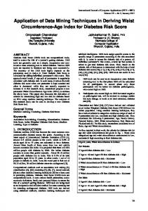
We are now ready to define the objective of data mining for association rules. Association rule mining [3] is: Given dataset D of objects and thresholds minsupp and minconf, find every rule X ⇒ Y so that support D (X ⇒ Y ) ≥ minsupp and confidence D (X ⇒ Y ) ≥ minconf . An association rule X ⇒ Y can be interpreted as “if a transaction contains X, then it is also likely to contain Y .” The thresholds minsupp and minconf are parameters that are specified by a user to indicate what sort of rules are “interesting”. Given the threshold minsupp, an itemset X is said to be frequent in a dataset D if support D (X) ≥ minsupp. Furthermore, a frequent itemset X is said to be maximal in a dataset D if none of its proper supersets is frequent. Clearly all subsets of a maximal frequent itemset are frequent. Also a frequent itemset X is said to be closed if none of its supersets has the same frequency. Figure 2 shows an example of mining frequent itemsets. Here we have a database of 5 transactions and the items bought in each. The table on the right hand shows the itemsets that are frequent at a given level of support. With a threshold of minsupp = 50% all of the itemsets shown are frequent, with ACTW, and CDW as the maximal frequent itemsets. An obvious approach to finding all association rules in a dataset satisfying the thresholds minsupp and minconf is the following: (1) Generate all frequent itemsets. These itemsets satisfy minsupp.
August 9, 2003
12:10
WSPC/Lecture Notes Series: 9in x 6in
Data Mining Techniques
Fig. 2.
zaki-chap
9
An example of frequent itemsets, where we use a threshold of minsupp ≥ 50%.
(2) Generate rules from these frequent itemsets and eliminate those rules that do not satisfy minconf. The first step above generally requires searching an exponential space with respect to the length of itemsets, and is thus computationally expensive and I/O intensive. Therefore, a key challenge in association rules mining is a solution to the first step in the process above. This problem has been studied by the data mining community quite intensively. One of the first efficient approach was the Apriori algorithm [3], which inspired the development of many other efficient algorithms[14, 35, 50, 58, 71, 73, 81]. Another promising direction was the development of methods to mine maximal [9, 15, 32, 49] and closed itemsets [59, 61, 83]. The Apriori algorithm [3] achieves its efficiency by exploiting the fact that if an itemset is known to be not frequent, than all its supersets are also not frequent. Thus it generates frequent itemsets in a level-wise manner. Let us denote the set of frequent itemsets produced at level k by Lk . To produce frequent itemset candidates of length k + 1, it is only necessary to “join” the frequent itemsets in Lk with each other, as opposed to trying all possible candidates of length k + 1. This join is defined as {i | i1 ∈ Lk , i2 ∈ Lk , i ⊆ (ii ∪ i2 ), |i| = k + 1, (6 ∃i0 ⊂ i, (|i0 | = k) ∧ (i0 6∈ Lk ))}. The support of each candidate can then be computed by scanning the dataset to confirm if the candidate is frequent or not. The second step of the association rules mining process is relatively cheaper to compute. Given the frequent itemsets, one can form a frequent itemset lattice as shown in Figure 3. Each node of the lattice is a unique
August 9, 2003
12:10
WSPC/Lecture Notes Series: 9in x 6in
10
zaki-chap
Zaki & Wong
Fig. 3. An example of a frequent itemset lattice, based on the maximal frequent itemsets from Figure 2.
frequent itemset, whose support has been mined from the database. There is an edge between two nodes provided they share a direct subset-superset relationship. After this, for each node X derived from an itemset X ∪ Y , we can generate a candidate rule X ⇒ Y , and test its confidence. As an example, consider Figures 2 and 3. For the maximal itemset {CDW }, we have: • • • • • • •
count D (CDW ) = 3, count D (CD) = 4, count D (CW ) = 5, count D (DW ) = 3, count D (C) = 6, count D (D) = 4, and count D (W ) = 5.
For each of the above subset counts, we can generate a rule and compute its confidence: • • • • • •
confidence D (CD ⇒ W ) = 3/4 = 75%, confidence D (CW ⇒ D) = 3/5 = 60%, confidence D (DW ⇒ C) = 3/3 = 100%, confidence D (C ⇒ DW ) = 3/6 = 50%, confidence D (D ⇒ CW ) = 3/4 = 75%, and confidence D (W ⇒ CD) = 3/5 = 60%.
Then those rules satisfying minconf can be easily selected.
August 9, 2003
12:10
WSPC/Lecture Notes Series: 9in x 6in
zaki-chap
11
Data Mining Techniques
X⊆T X 6⊆ T
Y ⊆T
Y 6⊆ T
TP FN
FP TN
Fig. 4. Contingency table for a rule X ⇒ Y with respect to a data sample T . According to the table, if X is observed and Y is also observed, then it is a true positive prediction (TP); if X is observed and Y is not, then it is a false positive (FP); if X is not observed and Y is also not observed, then it is a true negative (TN); and if X is not observed but Y is observed, then it is a false negative (FN).
Recall that support and confidence are two properties for determining if a rule is interesting. As shown above, these two properties of rules are relatively convenient to work with. However, these are heuristics and hence may not indicate whether a rule is really interesting for a particular application. In particular, the setting of minsupp and minconf is ad hoc. For different applications, there are different additional ways to assess when a rule is interesting. Other approaches to the interestingness of rules include rule templates [44], which limits rules to only those fitting a template; minimal rule cover [77], which eliminates rules already implied by other rules; and “unexpectedness” [51, 74]. As mentioned earlier, a rule X ⇒ Y can be interpreted as “if X is observed in a data sample T , then Y is also likely to be observed in T .” If we think of it as a prediction rule, then we obtain the contingency table in Figure 4. With the contingency table of Figure 4 in mind, an alternative interestingness measure is that of odds ratio, which is a classical measure of unexpectedness commonly used in linkage disequilibrium analysis. It is defined as T P D (X ⇒ Y ) ∗ T N D (X ⇒ Y ) θD (X ⇒ Y ) = F P D (X ⇒ Y ) ∗ F N D (X ⇒ Y ) where T P D (X ⇒ Y ) is the number of data sample T ∈ D for which the rule X ⇒ Y is a true positive prediction, T N D (X ⇒ Y ) is the number of data sample T ∈ D for which the rule X ⇒ Y is a true negative prediction, F P D (X ⇒ Y ) is the number of data sample T ∈ D for which the rule X ⇒ Y is a false positive prediction, and F N D (X ⇒ Y ) is the number of data sample T ∈ D for which the rule X ⇒ Y is a false negative prediction. The value of the odds ratio θ D (X ⇒ Y ) varies from 0 to infinity. When θ(X ⇒ Y )