Data
Mining
Association
Rules:
Takeshi IBM
Using
Tokyo
Scheme,
Fukuda
Research
IBM
Tokyo
co.jp
Research
Takeshi Tokyo
and
Morimoto
[email protected].
IBM
Optimized
Algorithms,
Yasuhiko
Laboratory
[email protected].
Two-Dimensional
Visualization
Shinichi
Laboratory
IBM
Tokyo
Morishita Research
Laboratory
morisitatltrl.ibm.co.
co.jp
jp
Tokuyama Research
Laboratory
[email protected]
Abstract
Association
We discuss numeric in
data
mining
attributes
a database
are two
of
numeric
attribute.
bank
on association
the pair
space,
and
rules
attribute.
customers,
attributes,
Taking
dimensional
based
and one Boolean
“Age”
(Age,
Balance)
we consider
Given a database universal relation, we consider the association rule that if a tuple meets a condition Cl, then it also satisfies another condition Cz with a probability (called confidence in this paper). We will denote such an association rule (or a rule, for short) between the presumptive condition (71 and the objective condition C2 by Cl + C2 1. Agrawal, Imielinski, and Swami [AIS93b] investigated how to find all rules whose confidences are greater than a specified minimum threshold, such as 50’Yo. They focus on rules with conditions that are conjunctions of (A= yes), where A is a Boolean attribute, and present an efficient algorithm. They have applied the algorithm to basket-clata-type retail transactions in order to derive interesting associations between items, such as
for two
For example, and
“CardLoan”
“Balance”
is a Boolean
as a point
an association
in two-
rule
of the
form ((Age, which
Balance)
implies
that
fall in a planar probability.
bank
region
and adrmssible
and
that
1
efficient
give optimal
= Yes),
whose ages and balances
to use card
loan
classes of regions, and z-monotone) algorithms
association
respectively.
for admissible
for visualizing
two
(i.e. connected
confidence,
algorithms
(CardLoan
customers P tend
We consider
each class, we propose regions
c P) *
regions,
We
with
regions.
rules for gain, have
a high
rectangles
for computing
For the
support,
implemented
and constructed
Rules
the
a system
(~i,zza = yes) A(~oke
= yes)
+
(potato=
yes).
the rules.
Improved versions of the algorithm have also been reported [AS94, PCY95]. In addition to Boolean attributes, databases in the real world usually have numeric attributes such as age and the balance of account in a database of bank customers. Thus, it is also important to find association rules for numeric attributes. In a companion paper [F MMT96a], we considered the problem of finding simple rules of the form
Introduction
Recent progress in technologies for data input through such media as bar-coded labels, credit cards, OCRS, and cash dispensers, have made it easier for finance and retail organizations to collect massive amounts of data and to store them on disk at a low cost. Such organizations are interested in extracting from these huge databases unknown information that inspires new marketing strategies. Current database systems are their primary means of realizing this aim, but in database and AI communities, there has been a growing interest in efficient discovery of interesting rules, which is beyond the power of current database functions [AGI+92, AIS93a, AIS93b, AS94, BFOS84, HCC92, NH94a, PCY95, PS91, PSF91, Qui86, Qui93, SAD+93].
(Balance
Permission to make digital/hard copy of part or all of this work for personal or classroom use is granted without fee provided that copies are not made or distributed for profit or commercial advantage, the copyright notice, the title of the publication and ifs date appear, and notice is given that copying is by permission of ACM, Inc. To copy otherwise, to republish, to post on servers, or to redistribute to lists, requires prior specific permission andlor a fee. SIGMOD ’96 6/96 Montreal, Canada Q 1996 ACM 0-89791 -794-4/96/0006, .,$3.50
13
E [VI, VZ]) +
(Car-dLoar2
= yes)
(*)
which expresses that customers whose balances fall in the range between VI and Vz are likely to use card loan. If the confidence of this rule exceeds a given threshold O (say, 10%), the range (i.e. interval) [VI, V2] r-ange of the numeric attribute is called a conjident value “Balance” with respect to the Boolean attribute “CardLoan.” Among a lot of confident ranges, we want to obtain one with high suppori (the number of tuples in the range). Fukuda et al. [F MMT96a] introduced some optimization
criteria
for
1We use the symbol %“ ship from logical implication,
finding
optimized
ranges,
that
in order to distinguish the relationwhich is usually denoted by “-”
effectively represent interrelation attribute and a Boolean one.
between a numeric
Two-Dimensional
Rules
Association
In the real world, binary associations between two attributes are not enough to describe the characteristics of a data set, and therefore, we often want to find a rule for more than two attributes. The main aim of this paper is to generate rules (which assoctatton rules) that reprewe call two-dimensional sent the dependence on a pair of numeric attributes of the probability that an objective condition (corresponding to a Boolean attribute) will be met. For each tuple t,let t[A] and t[l?] be its values for two numeric attributes; for example, t [A] = “Age of a customer t“ and t[l?]= “Balance of t“. Then, t is mapped to a point (t [A], t [1?]) in an Euclidean plane E2. For a region P in E2, we say a tuple t meets condition “(Age, Balance) E P“ if t is mapped to a point in P. We want to find a rule of the form ((A, B) E P) + C such as ((Age,
Balance)
G 1?) +
(CardLoan
Figure 1: Admissible
though there are many known algorithms for image segmentation, we need one that outputs an image region that generates a good (or, to be precise, an optimized) association rule. We consider two classes of geometric regions: rectangular regions, and admissible regions, which are connected x-monotone regtons. A region is called xmonotone if its intersection with any vertical line is undivided. Figure 1 shows an instance of admissible regions.
= yes).
In practice, we consider a huge database containing millions of tuples, and hence we have to handle millions of points, which may OCCUPY much more space than the
main
number
memory. of points,
distribute
the
equal-sized
To
values
buckets.
avoid
we discretize for
each
We divide
dealing the
with
numeric the
such
problem; attribute
Euclidean
We generalize an algorithm introduced by Asano et al. [AC KT96], which segments an object image from the background in a gray image, to our color-image case, and obtain a linear-time algorithm for computing the focused regton, which is the x-monotone region that maximizes the gatn (see section 2 for a definition). Although this algorithm uses sophisticated dynamic programming with fast mat;ix searching [AK M+87], we have confirmed experimentally that our implementation is fast not only in theory but also in practice. If we consider rectangular regions instead of x-monotone regions, the computation time for the optimal gain rule is increased to O(nl 5,, where n is the number of pixels in the grid. Next, we give efficient approximation algorithms for generating optimized support rules and optimized confidence rules (defined in later sections), through the use of focused regions.
a large
that
is, we into
plane
IV into
t N x N pixels (unit squares), and we map each tuple We use to the pixel cent aining the point (t [A], t [B]). a union of pixels as the region of a two-dimensional association rule. The probability that the tuples in a pixel (respectively, a region) satisfy the objective condition C is of the pixel (region). We would called the confidence region whose confidence is above like to find a conjident some threshold. The shape of region P is important for obtaining a good association rule. For instance, if we gather all the pixels whose confidence is above some threshold, and define P to be the union of these pixels, then P is a confident region with (usually) a high support. A query system of this type is proposed by Keim et al. [KKS94]. However, such a region P may consist of many connected components, and often create an association rule that is very difficult to characterize, and hence hard to see the validity. Therefore, in order to obtain a rule that can be stated briefly or characterized via visualization, it is required that P should belong to a class of regions that have nice geometric properties. Main
Region
Visualization
It is natural to visualize the region of a two-dimensional association rule ((A, B) E P) + C. Let us regard the region P as a color image on a grid G as follows: Let Ui,j and Wi,j denote the numbers of tuples and tuples satisfying the objective condition C’ in the (i, j)-th pixel G(i, j), respectively. The pixel G(i, j) has a color vector (w, , Ui,, –v$,J, O) in RGB space. This means that its red level is Vi,j, its green level is ut)~ – vt,j, and its blue level is O. Hence, the brightness level is ut,j, which represents the number of tuples that fall within the pixel. The confidence of each pixel is represented by its color; thus,
Results
The problem of extracting a confident region resembles that of image segmentation in computer vision. Al-
14
that 3.51% of customers have delayed their credit card payments at one time or another. By pushing the Query button, we can see a focused region enclosed in thick lines. The confidence and the support (the percentage of tuples in the region) can be found at the bottom of the window. By moving the slider, we can control the trade-off between the support and the confidence: if we move the slider to the left, the support increases while the confidence decreases. In response to such a movement, the visualization system recomputes the region together with its support and confidence. Our system is so fast that one can continuously move the slider and see how the region changes, as if one were watching a motion picture. In Figure 2, we can find a region with 14.1% of support and 12.8’%0of confidence, which is much higher than the average confidence. The shape of the region tells us the characteristics of unreliable customers. As a result, we can say “Unreliable customers, who have delayed payment of their card charges, can be characterized as relatively young people whose balance is low.” 2
Figure 2: Visualization
In this paper we consider association rules, which are stochastic relations between some conditions on tuples in a database. We consider some primitive conditions, and use them to describe more complicated conditions. For a Boolean attribute A, A = yes and A = no are primitive conditions. Our typical primitive conditions on numeric attributes A and B are A = v, A G 1, and (A, B) E P, where v is a value and 1 is a range in the domain of A, and P is a region of the product space of domains of A and B. Let Cl and C2 be conditions on tuples. An association rule (or a rule for short) has the form C’l + Cg. C2 condition, and Cl is called a is called an objecitve
system
redder pixel has a higher confidence. We construct a visualization system for our twodimensional association rules by reforming the color image introduced above, transforming it to make the rules easier for humans to grasp visually. We have tested our system, together with the functions given in our companion paper [F MMT96a], on some test database, and discovered several new simple rules, some of which seem to be of potential value to users in strategy planning. The database has about thirty numeric attributes and about one hundred Boolean attributes. Suppose that we select two numerical attributes, “Age” and “Balance,” and also a Boolean attribute, “Card Loan Delay,” for example. These attributes represent the ages of customers, the balances of their accounts, and whether they have delayed payment of their credit card charges, respectively. In order to characterize unreliable customers who have delayed payment, we consider the rule a
((.4ge, Baiance)
E P)
*
(CarctLoanDelay
Preliminaries
presumptive
condttion.
The support of condition C is defined as the percentage of tuples that meet condition C, and is denoted by support(C). In this paper, we normally denote the “number of tuples” that meet condition C rather than “percentage,” since we do by support(C) not want to declare the base of the percentage each time. The confidence of a rule Cl + C2 is defined C1), which is denoted by as support (C1AC2)/support( Conf(cl * C2). There are several types of association rules for attributes. Our first example is a rule where the presumptive condition is a primitive condition on a Boolean attribute.
= yes),
and find an optimized region of P. We divide data into sets of 20 x 20 pixels. Our visualization system shows an optimized region in those pixels as in Figure 2. The data has an average confidence of 3.5190, which means
Example 2.1 Consider a relation of basket-type retail transactions. Each attribute of the relation is a Boolean one whose domain is {yes, no}, and represents an item,
15
such as Coke
usually compress the data into N buckets B1, B2, . . . BN, by using an ordered bucketing so that for each t ~ B, and t’E Bj where i < j, t[A] < t’[A]. The number of tuples in Bi is denoted Ui, and the number of success tuples in B$ is W,. It is desirable that the buckets should be (almost) equal-sized; that is to say, tuples should be uniformly distributed into buckets. A fast method of performing such a bucketing is given in our companion paper [FMMT96a].
or Pizza. (Coke
= yes)=
(Pizza=
yes)
is an association rule. I The second example is a rule, which we call a oneassociation rule, where the presumptive condition is on a numerical attribute. dimenszonal
2.2 Consider a bank’s data on customers. Each tuple contains the balance of a customer at the bank and services, (card loan or automatic withdrawal, say) for the customer. Suppose that 5070 of customers whose balance is between 104 and 105 use credit card loans; then, we have the following rule, whose confidence is 50Yo:
From now on, we assume that we have equal-sized bucketing, and we only consider ranges each of which corresponds to a union of contiguously indexed buckets. For simplicity, we denote the range corresponding to B, U B,+ IU, ..., UBt by [s, t]. For a range 1 = [s, t], support(l) = ~~=$ Ui and hit(l) = ~~=, v, by if its confidence is not less definition. A rule is confident than a given confidence threshold $. A range generating range. A rule is a confident rule is called a confident ample if its support is not less than a given support threshold Z. A range generating an ample rule is called an ample range.
Example
(Balance
E
[104, 105]) ~ (CardLoan
= yes).
I The third example is a rule where the presumptive condition is a condition on two numerical attributes: Example 2.3 In a bank’s data consider another numeric attribute, following rule: {(Balance
c [104, 105]) A (Age
There can be many confident ranges, and we want to compute characteristic ones that optimize some criteria. gam range, Among them, let us consider the opttmtzed – 0 x support(I), which maximizes gaine (1) = hit(l) and the optimized support range, which is the confident range that maximizes support. We often omit subscript 9 if we fix the threshold.
on customers, we Age. Consider the
G
[40, 50])}
+ (CardLoan
= yes).
For example, let us consider the rule
I (Balance
The presumptive condition of the above association rule can be rewritten as a primitive condition (Balance, Age) c P, where P is a rectangular region [104, 105] x [40, 50] in the plane, which is the product space of the domains of Balance and Age. We call rules association rules, in which of this type two-dimensional P is not necessarily a rectangle (we will discuss this point later in detail). 3
One-Dimensional
Optimized
Association
and
suppose
100070
respect
the
Rules
that
gain
(CardLoan
the
of customers
optimized
from
E 1) +
credit use
range
the
credit
optimized for
the
card
credit
that
card
loan
support
customers
which loan
card
credit
is the
to the balance)
loan
card range
system
bank
pays
Then,
of customers
system. is
(y)
loans.
maximizes
range the
= yes)
(with
the bank’s On
the
does
the
other
largest not
lose
if the
profit hand,
range money
of on
system.
are the optimized In Figure 3, l(gain) and I(support) gain and the optimized support ranges in which the confidence threshold is 0.4. l(con~idence) is called the optimized confidence range, which is the ample range that maximizes the confidence (in this example, the support threshold is 200).
Ranges
It is important to mine association rules whose confidence is high, and whose support is sufficiently large. In this subsection, we define optimization criteria for the range 1 in a one-dimensional association rule (A E 1) + and C is a fixed C, where A is a fixed numeric attribute objective condition. For simplicity, we write support(l) E 1), and hit(l) for suppori((A E l)AC), for support(A which are called the support and hit support of I, respectively. For a tuple t, we define t[A] to be the value of A at t.A tuple is called a success tuple if the condition C holds for it. Since there are often too many tuples in a large database to be accommodated in main memory, we
In this paper, we consider the optimized gain range, give a linear (O(N)) time algorithm for computing it, and generalize it to two-dimensional cases. 3.1
From
“Programming
Pearls”
In the “Programming Pearls [Ben84]” column of CACM, J. Bentley presented a problem for demonstrating importance of efficient algorithms in program design. The problem is:
16
~
50
50
50
50
50
50
50
50
50
50
50
50
50
v
12
16
30
26
13
21
15
33
13
9
11
22
12
between 400 and 250000. For simplicity, we assume that N~ = NB = N from now on, although this assumption is not essential. For a set, of pixels, the union of pixels in it forms a planar region, which we call a ptxei reg~on. A pixel region is x-monotone if its intersection with each column is undivided (thus, a vertical range) or empty. A connected and x-monotone region is called an admtsstble regton.
X(-confidence)
Figure 3: Optimized
For each tuple t, t[A] and t[B] are values of the numeric attributes A and B at t. If t[A] is in the i-th bucket and t[l?] is in the j-th bucket in the respective bucketing, we define f(t) = G(i, j). Then, we have a mapping ~ from the set of all tuples to the grid G. For each pixel G(i, j), u~,j is the number of tup~es mapped to G(i, j), and V,,J is the number of success tuples mapped to G(i, j). Given a region P, define support(P) = ~~(i,J)~P U,,j. and hit(P) =
Ranges
“Given a list X of .V real numbers, compute the maximum sum found in any contiguous subvector of it.” This problem is equivalent to our problem of computing the optimized gain range. Given a confidence threshold d, we define a list X so that X(i) = vi – t? x u,. Then, .Y[s, f] is the solution of the problem if and only if [s, t] is the optimized gain range. Bentley introduced four algorithms, whose time complexities are 0(N3), 0(.V2), O(Nlog N), and O(N), respectively. The linear time algorithm ( Kadane’s algorithm) scans the data with respect to the array ind~x. For each i,
The following
two
IMcm(i + 1) = mu{ O,lfaz(i)} + X(i + 1), and kfaz(~ i + 1) = max{A4a.r(i + l), fkfaz(~ i)}. Thus, a simple dynamic programming time solution. Therefore, we have the following: Theorem
3.1
tn O(N)
ttme.
4
The
Two-Dimensional
Problem
opttmtzed
gain
gives an O(N)
range
Association
can
0, we define g(8)ij
=
optzmtzed gatn rule (f(t) E P) ~ C, where P is the admissible region that maximizes gain(P). The region gatn admzsstble regton. is called an opttmued lNote that, there may be more than one optimized gain admissible regions associated with a given threshold O. In such a case, we compute both the optimized gain admissible regions with the maximum support and the minimum support. As in the case of ranges, we call a region confident (resp. ample) if its confidence (resp. support) is at least a given threshold value. Similarly, we define an optzmtzed support admissible regton, which is the confident and admissible region that maximizes support, and optimued confidence admwwble regzon, which is the ample and admissible region that maximizes confidence. Instead of admissible regions, the rectangular subreis called the opgion W of G that maximizes gain(W) rectangle. t~mized gain (support, confidence) Note that, if we want to find the connected pixel region with the maximum gain, rather than an admissible region or rectangle, the problem becomes N P-hard, in line with a similar argument to that by Garey and Johnson [GJ77] for the grid Steiner tree problem.
A4az(i) = max, $i X([S, i]), and .!~a.r(< i) = max$~~~~ X([s, t]).
Then, Jfaz(s N) is the answer. relations are easy to see:
Given a threshold
~G(i,j)~Pv~j
– 0 x support(P) = ‘ll~,j – Oui,j, and gain(P) = hit(P) We want to find the two-dim ens~onal ~G(i,j)~Pg(Ol~,j
be found
Rules
formulation
Let us consider two numeric attributes A and B, and an objective condition C. We distribute the values of A and B into NA and NB equal-sized buckets, respectively. Let us consider a two-dimensional NA x NB pixel-grid G, which consists of NA x NE unit squares called ptxels. G(i, j) is the (i, j)-th pixel, where i and j are called the row number and column number, respectively. The jth column G(*, j) of G is its subset consisting of all pixels whose column numbers are j. Geometrically, a column is a vertical stripe. We use the notation n = NA x IVB. In our typical applications, the ranges of NA and NE are from 20 to 500, and thus n is
Algorithms
for
computing
optimized
rectangles
are 0(N4 ) rectangular subregions of G. Thus, a naive algorithm computes the gain of each of these O(N4) rectangles and outputs the one with the maximum gain. The time complexity of this algorithm is 0(N5) = 0(n2 5), which is too expensive. It can be easily reduced to to O(nl 5, by using Theorem 3.1, as follows: We choose a pair r < T’ of rows in G, and consider only rectangles whose horizontal edges are on these rows. For each column index j, we compute the sum There
17
x(j)
=
in any
~~~r
g(~)i,j,
contiguous
in Programming with
the
time. ‘The
Pearls).
maximum
Since
time
and
same
time
for
special
candidate
algorithm
complexity
maximum
X()
we obtain
this
are 0(N2) of the
the
of the list Thus,
gain
there
complexity
compute
subvector
can
sum
(the
problem
the
rectangle
case in
pairs
=
be found
in
Lemma
Further
improvement
Similarly, al.
by using
[FMMT96a]
ranges pute
problem
and the
linear
for
time
time
complexity
the
confidence support
confidence
rectangle
Theorem
4.1
confidence
rectangles can be computed
Each
and
we
Fischer
et
is given
et
support com-
the optimizeq
in
support,
for computing region
O(nl 5, time.
an optimized
are
maxi-
tndices
topm(s)
can be computed
and
bottomm(s)
in O(N)
for
time.
+1, j+l)2M(i,
j+l)+Ll(i+
1,~)
for every 1< i < j+ 1< N. It is well known [AKM+87] that all locations of the row maxima of this matrix can be computed in O(N) time (of course, we cannot afford to construct the matrix in order to obtain this time complexity). By definition, the location of the maximum entry of the s-th row is topm (s). Thus, we can compute all topm(s) (s = 1, 2, ... N) in O(N) time. The computation of bottomm (s) is analogous. ~
and
This time complexity is a little more expensive than that for the optimized gain admissible regions (see the next subsection), and thus a data mining system using rectangles is considerably slower than one using admissible regions. Furthermore, in our experience, the use of non-rectangular regions often yields useful rules. as the For example, let us consider “Age” and “Salarfl numeric attributes, and “GoldCard” as the objective condition. Here, we would expect to find a rule that, among people on the same salary, younger ones are more likely to pay an annual fee for premium credit cards. This expectation is confirmed if we find a twodimensionai association rule whose region resembles a triangle, which is an admissible region, but (of course ) not a rectangle. Consequently, we believe that admissible regions are better than rectangles for our class of regions in two-dimensional association rules. Algorithm admissible
The
, ... N
Lf(i, j)+lM(i gain,
g(u~
Let us define Sum~(l) = ~i~~ g(~),,~ for each integral subinterval 1 of [1, N]. Then, an inequality Summ(l) + Summ(l’) ~ Summ(l n 1’) + Summ(l U 1’) holds if 1 n 1’ # 0 (indeed, equality holds). This inequality is often called the Monge inequahty. Define an N x N matrix M whose (k, 1)-th entry is Sum~([k, 1]) Because if k ~ 1, and negative infinity otherwise. of the Monge inequality, the matrix becomes a totally matrix, that satisfies monotone
time.
of the opttmtzed
Xp.m(’)
Proof:
[Ben84].
can
and
the
0(n15).
of Fukuda
optimized
ranges,
rectangle
in 0(n15)
Pearls
algorithms
computing
optimized
optimized
of this
in Programming
4.1
a11s=l,2
al. [FHLL93].
as a research
g(m~
mized, respectively.
O(N)
of rows,
is 0(iV3)
Iibommzm(.)
For two indices s and s’, we define coverm(s, s’) to be Sum[bottomm(s),
topm (s’)]
Sum[bottom~(s’),
top~(s)]
if s s s’, and ifs > s’.
Let G(*, < m) be the part of the grid on the left of the m-th column, including G(*, m). We define 17(i, s m) to be the maximum gain of admissible regions that contain the pixel G(i, m) and are contained in the region G(*, s m). Then, we have the following formula: F’(i, ~ m+l)
= ~~,~x~{F(j, ——
< m)+covern+~(i,
j)}
(**)
or Oif the above value is negative. From this formula, we can compute maxm{maxl f’(i, s m)} and the associated region, which must be the optimized gain region.
gain
Lemma we can
Since the intersection of an admissible region with a column is an interval, it would appear that if we compute the maximum gain range in each column and compute their union, we can compute the optimized Unfortunately, this region gain admissible region. is often disconnected, although the connectivity of a region is very important for creating a good rule. The following algorithm is essentially the same as that given by Asano et al. [ACKT96] for solving an image segmentation problem. However, to the best of our knowledge, this is the first case in which an algorithm using “fast matrix searching” [A KM+ 87] routines has been implemented in a database system. For each m = 1,2, ... N, we pre-compute the indices bottomm(s) and topm(s) for all 1 ~ s < N, are defined so that where bottomm (s) and topm(s)
O(N)
4.2
If F’(j,
compute F(i, time.
<