Monitoring sensors is significant for vehicle fault detection and diagnosis. ..... 419,2003. [5]. T. Denton, âAdvanced Automotive Fault Diagnosis,â Butterworth-.
Data Reduction and Clustering Techniques for Fault Detection and Diagnosis in Automotives Aurobinda Routray , Associate Professor, Aparna Rajaguru, Research Consultant Department of Electrical Engineering IIT Kharagpur, India West Bengal 721 302,
Satnam Singh Senior Researcher - Diagnosis & Prognosis Group India Science Lab, General Motors Global R&D GM Technical Centre India Pvt. Ltd, Creator Building, ITPL Whitefield Road, Bangalore - 560 066, INDIA
`
Abstract— In this paper, we propose a data-driven method to detect anomalies in operating Parameter Identifiers (PIDs) and in the absence of any anomaly, classify faults in automotive systems by analyzing PIDs collected from the freeze frame data. We first categorize the operating parameter data using automotive domain knowledge. The dataset thus obtained is then analyzed using Principal Component Analysis (PCA) and Independent Component Analysis (ICA) for finding coherence among the PIDs. Then we use clustering algorithms based on both linear distance and information theoretic measures to assign coherent PIDs to the same class or cluster. A comparative analysis of the behavior of PIDs belonging to the same cluster can now be made for detecting anomaly in PIDs. Since a system fault is characterized by the values by of all PIDs across all the clusters, we use the joint probability distribution of the independent components of all PIDs to characterize the fault and find the divergence between the joint distributions of training and test data to classify faults. The proposed method can analyze available parameter data, categorize PIDs into informative or non-informative category, and detect fault condition from the clusters. We demonstrate the algorithm by way of an application to operating parameter data collected during faults in catalytic converters of vehicles.
I.INTRODUCTION
A
modern automobile contains a large number of modular subsystems. The health of these subsystems is typically monitored via a few thousand operating Parameter Identifiers (PIDs) which are continuously collected using various sensors and diagnostic software routines contained in the on-board Electronic Control Units (ECUs). The ECUs are the key components of an automobile and contain diagnostic software to process the sensory data and generate a fault code or Diagnostic Trouble Code (DTC) in case of a fault or malfunction of a major component. However, the number of DTCs is limited in a vehicle and finding the root cause becomes difficult if several DTCs are triggered simultaneously. Also, the DTCs may not be very conclusive about a specific fault because they are generated in several operating conditions and based on numerous sensor outputs. Therefore, the operating parameters identifiers (PIDs) need to be analyzed off-board in a holistic manner to find the root cause of the problem. Additionally, we can define the effectiveness of the diagnostic routines based on the accuracy and reliability of the related PIDs.
II.REVIEW ON DATA-DRIVEN FAULT DIAGNOSIS The modern automotive systems are too complex to build a vehicle-level physical model. Hence, the data-driven method is an alternative approach for fault detection and diagnosis. In addition, data-driven approach is advantageous as it is flexible and doesn't require a detailed physical knowledge of the system. Monitoring sensors is significant for vehicle fault detection and diagnosis. Dunia et al. described a data- driven method for sensor fault diagnosis using a model based on Principal Component Analysis (PCA) that partitions the measurement space into two orthogonal subspaces: the principal subspace for normal variations and the residual subspace for noise and abnormal variations [1]. The measurement vector is decomposed into orthogonal vectors by projecting it onto these subspaces. In case of a fault, a change in correlation among the variables increases the projection onto the residual subspace to unusual values as compared to those obtained during normal conditions. Yu et al. have proposed a Radial Basis Function Neural network (RBFN) for sensor fault detection in a chemical rector process [2]. We propose a novel data-driven methodology to systematically analyze the operating parameter data to detect anomalous PIDs and in the absence of any anomaly, classify faults in automotive systems i.e. decide whether the fault described by the test data belongs to the modeled fault described by the training data. We demonstrate this methodology by way of an application to operating parameter data collected when faults occurred in the Heated Oxygen Sensor (HO2S) of the catalytic converter system. Anomaly detection and fault identification is achieved in two steps. Step1: Constructing Clusters of Coherent PIDs (Training Phase). a) First we categorize the operating parameter data using automotive domain knowledge and further exclude PIDs that have very low variance. b) The data is then analyzed for coherence across the various PID values using data reduction techniques which utilize correlation and information-theoretic measures. b) Clustering is performed where coherent PIDs are assigned into the same cluster. c) For characterizing the fault in HO2S system that is under consideration, the joint probability distribution of PIDs across clusters is estimated.
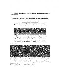
In the training phase, we assume that all the PIDs in the dataset are authentic i.e. without anomaly and hence can be used for formation of clusters as well as describing the fault by fitting a joint distribution. Step2: Detecting Fault (Testing Phase) a) When an unknown set of PIDs need to be analyzed, the pattern is treated in clusters as formed in Step.1. b) The anomalies in a PID can be detected by measuring the statistical distances of that PID from others in the same cluster and comparing the distribution of these distances with those obtained from the past data as in Step1. If the distances are similar then the PIDs are authentic for fault classification. Fault classification is performed after removing the anomalous PIDs. c) Fault classification has been carried out by estimating the divergence between the joint probability distributions of the PIDs observed from the vehicle under test with that of the joint probability distribution found as in step-1 from the historical data. III. DESCRIPTION OF OPERATING PARAMETERS DATA We employ operating parameter (PIDs) data of a catalytic converter system. A catalytic converter is a key component of the engine exhaust system and treats the exhaust gases before emitting into the atmosphere. The converter reduces carbon monoxide, un-burnt hydrocarbons, and also oxides of nitrogen and hence is known as three way converter [3] [4]. The HO2S senses the output of the catalytic converter and develops a voltage by comparing the oxygen level in the output of the catalytic converter and the atmosphere. The output of the oxygen sensor is used for post catalyst monitoring as well as for regulation of fuel control [5]. In our data experiments, the operating parameter data contains 296 parameter identifiers (PIDs) collected for the same fault. The PIDs data comprises of quantitative as well qualitative information which needs to be preprocessed using the domain knowledge and data reduction techniques. Some dependency among the PIDs can be deduced from automotive domain knowledge. The unknown dependencies among the PIDs can be learned by computing the correlation and information-theoretic distances between them. IV.THE FAULT DETECTION METHODOLOGY From the initial dataset, we eliminate PIDs irrelevant to the fault using automotive domain knowledge. We further exclude PIDs that are constant valued or have inappreciable variance. Training Fig.1 shows the flowchart for the proposed method in the training phase to process the PIDs data to a state where we can have trainable classifiers for diagnosis. Step 1. (Finding Data Redundancy): One of the key assumptions in our methodology is the presence of
Operating Parameters Data Data reduction using automotive domain knowledge & exclusion of PIDs with negligible variance
training dataset
testing dataset
Estimation of the number of clusters Clustering Characterization of fault being modeled by fitting a joint probability distribution function Fig.1 Flowchart of the training stage
coherence among the PIDs. Coherence justifies forming clusters of the coherent PIDs such that PIDs in the same cluster have similar variation due to their coherence. In this step, we apply Principal Component Analysis (PCA) and Independent Component Analysis (ICA) for reducing the data size and finding the coherence among the PID values. Principal Component Analysis (PCA): PCA identifies a linear combination (Principal Component) of variables that best describe the variability in the dataset. The Principal Components (PCs) are calculated by the eigenvector decomposition of the covariance matrix of the PIDs data. PCs which describe the most variability e.g. 90% of the total variance in the dataset are used as basis vectors for transforming the data into a new reduceddimensional space. This enables us to extract information about the redundancy in the dataset. Further, PCA is effective only under the assumption that the data has Gaussian distribution which may not be true for automotive systems because there are several nonlinear processes which could generate non-Gaussian data. Independent Component Analysis (ICA): ICA is a non-linear technique to estimate statistically independent components from a data matrix. We want to use ICA for linear representation of non-Gaussian data so that the components are statistically independent, or as independent as possible. Independence is a more stringent condition than the un-correlatedness that is imposed by PCA. Hence, ICA would be more effective in our application because automotive subsystems are highly nonlinear and data is more likely to be non-Gaussian [6], [7]. Since we have already reduced the data by PCA, we applied ICA on the PCA output to check if any further reduction is possible.
The redundancy discovered by PCA and ICA shows the coherence present amongst the PIDs which can be utilized for fault detection in two approaches: 1) we could reduce the number of PIDs and form a data set with several-fold reduction in data size 2) we could divide the PIDs data into as many clusters as the number of independent components. The second approach helps us in identifying anomalous PIDs by checking its statistical deviation with its expected cluster. We describe the details of this approach in next step. Step 3. Clustering: Clustering is an unsupervised method of classifying the unlabeled PIDs dataset into finite “hidden” data-structures depending on their proximity in some feature space [8]. Here, the PIDs data is unlabeled because we don't know the faults before the analysis. Clustering involves selection of distinguishing features from a set of candidates and then transforming them to generate novel features from the original ones (proximity measures). The samples are then clustered according to their proximity in the transformed feature space. Once a proximity measure is chosen, the construction of a criterion function makes the partition of clusters an optimization problem. The optimality of the clustering process can be verified by Silhouette [9] plot that measures the Silhouette width of a PID is a cluster. The Silhouette width is defined as ��� =
(�� � ) �( � ,�� )
(1)
where ��� is the Silhouette width, �� is the average dissimilarity of the � �� point from all other points in its own cluster and �� is the minimum of the average dissimilarity of it from all other clusters present. ��� varies from 1 (good clustering) to -1 (inferior clustering). Clustering can be performed based on either distance measures or mutual information measures between the PIDs in the corresponding clusters. Clustering based on distance or similarity measures: Choice of the dissimilarity measure is problem dependant. The most commonly used distance measure is the ‘Euclidean’ distance .The drawback of distance measures is that the largest scaled feature tends to dominate other features [8]. Hence, we need to normalize the data before clustering. A comparison between syntactic and statistical measures of data clustering suggests that the later outperforms the former [10] [11]. Clustering based on Mutual Information [6]: The entropy H(V) of a random variable defined on a dataset is a measure of the average amount of information about the data that is contained in V. Formally it is defined as (2) H (V ) = − p(vk ) log2 p(vk )
∑ k
where p (vk ) is the probability of V having the kth value vk in the data set. If W is another random variable described on
the same dataset, then the Mutual Information (MI) between the random variables V and W is given by
I (V ;W ) = H (V ) − H (V | W )
(3)
H (V | W ) is the conditional entropy of V after W has been observed. Since H (V ) is the uncertainty associated with V before any observation has been made, MI is a measure of the uncertainty about V that has been resolved by the observation of W. Thus, MI is a measure of the mutual dependence between V and W. In our context, if two PIDs have a high value of MI, it implies that they have a high degree of dependence among them. We find the MI between each pair of PIDs and the ones that have a high value of it are grouped together. This helps in knowing the groups of PIDs that are coherent with each other. The distribution of the similarity (MI) of these PIDs in a cluster is the knowledge gained from it. There are as many distributions as there are clusters. Step 4: Characterizing the fault by fitting Joint probability distribution to the PIDs as a whole: The state of the system under fault is described by the values of the PIDs and hence is a function of all PIDs across all clusters. As a pre-requisite for fault classification, we find the joint probability distribution of the independent components of all PIDs in the training phase. Fault classification can be done by finding the KulbackLeibler divergence (KL divergence) between the joint probability of the independent components in the training set PIDs and that of the PIDs in the testing set. The KL divergence quantifies the proximity between two probability distribution functions. It is defined as ��� (�||�) = ∑� �� ���� where � = {�� } distributions.
and
� = {�� }
�
(4)
!�
are
two
probability
The Fault Detection Process (Testing):Let us assume that a DTC is triggered during the operation of the vehicle, thus indicating the occurrence of a possible fault. As mentioned before, the generation of a DTC may not always point out the root cause as they are generated based on a diagnostic routine which follows certain logical or hard decisions. However, we can detect the anomalies by analyzing the PIDs in clusters formed previously in the training phase. The PIDs in a cluster are coherent. Hence, any variation in one parameter should be accompanied by similar variations in all other coherent parameters under nominal conditions. The distance and mutual information between these PIDs should remain the same for any later instance of the fault.
Operating Parameters Data from the test dataset Comparison with PIDs in the same cluster
No
Is
Yes
deviation high?
Fault classification by comparison of joint probability distributions
The PID is not authentic
Is divergence Yes high? Fault is not of Fault belongs to modeled class modeled class No
Fig.2 Flowchart for Training stage
If any of the PIDs is anomalous, then it will not remain coherent with other PIDs in its cluster and the distance of this PID with respect to others in the same cluster will differ from its previously estimated values. To detect an anomaly, we project the MI of that PID with respect to others in the same cluster on the distribution of that cluster estimated in the training phase. If the projected values are high, then we conclude that the PID is not anomalous whereas a low values indicate anomaly in the PID. If we know the sensor from which a particular PID is derived, then we can infer that a particular sensor might be faulty by the detection of anomalous PIDs. However, in this paper we are mainly concerned with classification of faults and hence restrict the method to simply detect the presence of anomaly in PIDs. If any anomalous PIDs are present, then fault classification cannot be made. However, when all the PIDs in a cluster are good, then fault classification can be made by finding the divergence between the joint probability distribution of the independent components of historical data characterizing the fault and the PID values being tested. A low divergence between the two faults indicates a fault belonging to the modeled class. V. RESULTS AND DISCUSSION To demonstrate the proposed methodology, we have considered faults in HO2S heater control circuit bank, HO2S heater performance bank and HO2S heater resistance circuit bank in 1376 patterns. The resulting dataset has dimensions 1376×253 where the number of PIDs is 253 consisting of both binary and real-valued PIDs. From these, 42 PIDs were selected using the domain knowledge. The resulting dataset has dimensions of 1376×42. From this we selected 33 PIDs having high variance for analysis. The data set consisting of 1376 patterns was divided randomly into a training set of 900 patterns and a testing set of 476 patterns.
Data Reduction and Redundancy checking: The training dataset was examined for redundancy using both PCA and ICA methods. In PCA, the orthogonal directions along maximum variation (Principal Components) were identified. In the Scree plot [8], it was observed that a significant knee occurred at the 9th principal component (Fig.3) and the first 9 components were calculated to account for more than 85% of the total variance in the dataset. This implies that the data from the PIDs show major variation along 9 orthogonal directions. Going by the assumption that Principal Components with larger associated variance represent interesting structure and those with lower variation represent noise, we can infer coherence in the data. This inference is further validated by Independent Component Analysis. Since independence is a stricter constraint than uncorrelatedness, the components identified under PCA are further processed using ICA and the entropy of each latent independent component so determined was estimated. Out of 9 only 7 components are found to be significant by ICA. This step shows that there is redundancy in the PIDs data and it could be analyzed via clustering. Next, we perform clustering to find the actual number of clusters and their consistency to represent the original data. Clustering: The training dataset was again divided into 3 parts of 300 patterns each for confirming the cluster formation. Initially, the PIDs are divided into 7 clusters corresponding to the 7-independent components obtained from the data reduction method discussed above. During repetitive testing across the 3 data sets, it was observed that certain PIDs remained isolated from the other clusters. This condition remained even when process was repeated with Euclidean and Seuclidean (Standardized Euclidean) distance measures indicating that there are no PIDs in the dataset that are coherent with these PIDs. We detected 8 such PIDs in the dataset. These PIDs were separated from the original dataset and the new dataset so formed is again clustered by syntactic methods using distance measures to obtain 5 clusters which are nearly identical in the three data sets. To obtain more accurate results, we repeat the clustering with statistical measures. The MI between PIDs in three individual data sets is estimated and the PIDs are grouped into 5 clusters based on them. The PIDs in each cluster are now completely identical in the three datasets. Fig.4 is the Silhouette plot for clusters based on mutual information between the PIDs. In the figure, each horizontal bar corresponds to a PID and every contiguous set of bars represents a cluster. The length of a bar is a measure of the tendency of that PID to belong to the cluster it is in. PIDs in a cluster are coherent. This implies that that parameters indicated by PIDs in one cluster have similar trends in variation. If the PIDs are not erroneous, any change in one parameter should be accompanied by similar variations in all other parameters.
Dataset 1
15
Dataset 2
1
Dataset 3
1
1
0 0
5
10
15 20 eigenvalue index
25
30
35
Fig.3: Scree Plot
Hence, the mutual information among the PIDs should have similar distributions in both historical and testing data sets in the absence of any anomaly in the PIDs. We adopt the clusters using Mutual Information measure to characterize the coherence amongst the PIDs. The distribution of this coherence is further characterized by fitting the density functions for each cluster (Fig.5).Now we follow the method outlined in Section-4 for fault detection. We chose data sets from 476 patterns marked for testing. Case-1 (No Anomaly in the PIDs) We randomly choose 50 of the 476 patterns for testing. The test results can be divided into two parts. In the first part we check the cluster distributions for detecting any anomaly or error in the PIDs. If there is no anomaly then the PIDs are authentic and we can proceed to the second part i.e. fault classification. Here, we find the KL divergence between the joint probability distributions of the modeled fault and test data. Detection of Anomalous PIDs We measure the MI of the PID being tested for anomaly with respect to others in its cluster and project these values into the already computed distributions (Fig.5). We use here the PID-values of Mass Air Flow (MAF) sensor output as an example. This PID remains in cluster-1 which has 12 different PIDs. First, we compute the mutual information of MAF sensor output PID value with respect to the 11 other PID values and then project each of them to onto the distribution function of MAF cluster-1 obtained previously during training(Fig. 5). The process is repeatedly performed by selecting random sets of 50 patterns each time. Fig.7 (a) shows the plot of the values obtained by projection versus the corresponding mutual information of this PID with respect to the other PIDs as the MAF cluster-1 for 50 patterns. The estimated values are high. This implies that the distances (MI) of this PID with respect to other PIDs in cluster 1 in the test data is similar to those in training data and hence it is varying in coherence between with other PIDs in cluster 1. Hence, the PID is not anomalous. This process has to be repeated for all PIDs in the dataset. Fault Classification: Since the DTCs were triggered for a particular group of faults, the fault is characterized by the PID values in the
Cluster
2
2
2
3
3
3
4
4
4
5
5 0
0.5
1
5 0
0.5
1
0
0.5
1
Silhouette Fig.4Value Silhouette Silhouette with MutualValue Information Silhouette measures Value Distribution function for cluster 1
5
Cluster
Cluster
eigenvalues
10
2.5 2 1.5 1 0.5 0 0
0.2
0.4 0.6 0.8 1 1.2 Similarity using Mutual Information
1.4
Fig.5 The Distribution Function of Similarity Measures using Mutual Information for Cluster 1
training set. During the testing phase, any set of PID values of that fault should have a similar joint probability distribution function of their independent components and KL divergence between the distributions of PIDs during the hand, a different fault would result in a different joint probability distribution function and the divergence between the two distributions would be high. We find the KL divergence between the joint probability distribution of independent components of the historical training data and test data for faults in HO2S (modeled class) and for faults that do not belong to this class for fault classification. The KL divergence is higher in the later case i.e. greater than 14 (Fig. 6(b)) as compared to the former i.e. less than 10 as is depicted in Fig. 6(a). Hence, large values of divergence indicate fault not belonging to the modeled class. Case-2 (case of anomalous PID) To test the clusters, we deliberately add random noise to the MAF sensor PID. We repeatedly test it as in Case-1 and obtained the graph as in Fig.7 (b) in which the values obtained by projection are low. This implies that the PID is no longer varying in coherence with its cluster and hence is anomalous. As the PIDs are erroneous, fault classification is not possible. VI. CONCLUSION In this paper, we have proposed a data-driven framework to systematically detect faults in automobiles. In principle, the clustering approach has been utilized to study the coherence among the various PIDs and use this coherence for diagnosis of faults.
frequency count
10
5
frequency count
0 10 15 20 25 30 35 40 45 KL Divergence between joint probability distributions of training and testing data for faults not belonging to the modeled class Fig.6(a) 20 15 10 5
0 0 2 4 6 8 10 KL Divergence between the joint probability distributions of training and testing data for faults belonging to the modeled class Fig. 6(b)
projected values using cluster 1 distribution function
ACKNOWLEDGMENT This work was supported by the GM India Science Lab, Bangalore, India. We would like to acknowledge Halasya Siva Subramania for his help on transforming the PIDs data. We are also thankful to Pulak Bandyopadhyay and GM India Science Lab technical committee for their valuable suggestions and feedback which improved the quality of this paper.
Fig.6 the KL divergence between joint probability distribution of training and testing datasets 2 1.5 1
REFERENCES
0.5 0 0
0.2 0.4 0.6 0.8 1 1.2 similarity measure of MAF sensor with respect to other PIDs in cluster 1
1.4
Fig. 7(a) Good MAF PID 0.5 Projected values using cluster 1 distribution function
While constructing the clusters, the basic assumption is that the training data has no erroneous PIDs and that the DTC always indicates a fault. The clusters are described by the distribution of MI among the PIDs. Further, we have constructed a joint distribution of independent components of the PIDs as a whole to describe the fault being modeled. We have implemented the algorithm on a set of PIDs collected during faults in the HO2S circuit in the catalytic converter. The anomaly detection process could identify anomaly in the MAF sensor when we added random noise to the PID values. In the absence of anomaly in any of the PIDs, the method could also decide whether the fault being tested belonged to the modeled class of faults in the HO2S. The clusters and distributions are true for a group of faults which fall under the specific DTC and might need to be constructed for other faults as well. This method works only when there are at least two PIDs in a cluster. Future research shall focus on combining qualitative information from Subject Matter Experts (SMEs) with the statistical tools to project the PIDs into lower dimensional space. We also plan to work on enhancing the PIDs dependency analysis using higher order information theoretic measures.
0.4 0.3 0.2 0.1 0 0
0.05 0.1 0.15 0.2 Mutual Information of MAF PID with respect to PIDs in cluster 1
Fig. 7(a) Faulty MAF PID Fig.7 The projection of Mutual Information of MAF sensor with respect to other PIDs on the distribution function of Cluster-1 for 50 patterns
0.25
[1]. R. Dunia and S. Joe Qin, “Joint diagnosis of process and sensor faults using principal component analysis,” Journal of Control Engineering Practice, vol. 6, pp. 457-479,1998. [2]. D. L. Yu, J. B. Gomm and D. Williams, ”Sensor fault diagnosis in a chemical process via RBF neural networks,” Control Engineering Practice, Volume 7, Issue 1, pp 49-55, January 1999. [3]. R .J. Farrauto and R. M. Heck, Catalysis Today 51, 1999, pp.351. [4]. J. Kasˇpar, P. Fornasiero and N. Hickey, Catalysis Today 77, pp. 419,2003. [5]. T. Denton, “Advanced Automotive Fault Diagnosis,” ButterworthHeinemann Publication, pp. 92-93, 2006. [6]. S. Haykin, “Neural Networks: A Comprehensive Foundation”, McMaster University, Prentice Hall, ch.10,1999. [7]. N. Das, A. Routray and P. K. Dash, "ICA methods for blind source separation of instantaneous mixtures: A case study", Neural Information process. Letters and Reviews, vol. 11, no. 11, pp. 225-46, Nov. 2007. [8]. R. Xu, and D. Wunsch II, “Survey of Clustering Algorithms”, IEEE Transaction on Neural Networks, vol. 16, no. 3, pp. 645-678, May 2005. [9]. W. L. Martinez and A. R. Martinez, “Exploratory data analysis with Mat lab,” Chapman & Hall/CRC, 2005. [10]. A. K. Jain, M. N. Murty, and P. J. Flynn., “Data clustering: A review”, ACM Computing Surveys, pp 264–323, 31(3) 1999. [11]. E. Tanaka, “Theoretical aspects of syntactic pattern recognition,” Pattern Recogn. 28, pp 1053–1061, 1995.