Suppose each edge e has a real-valued cosi c(e). The cost c(S) of ... ity matching
is a matching with the greatest number .... using a data structure of [G85b]. This.
Chapter
46
Data Structures for Weighted Matching and Nearest Common Ancestors with Linking Harold
N. Gabow*
Abstract. This paper shows that the weighted matching problem on general graphs can be solved in time O(n(m + n log n)), f or n and m the number of vertices and edges, respectively. This was previously known only for bipartite graphs. It also shows that a sequence of m nca and link operations on n nodes can be processed on-line in time O(ma(m, n)+n). This was previously known only for a restricted type of link operation.
optimization; detailed discussions are in [L, LP, PS]. Edmonds gave the first polynomial-time algorithm for weighted matching [El. Several implementations of Edmonds’ algorithm have been proposed, with increasingly fast running times: O(n3) [G73, L], O(mn log n) [BD, GMG], O(n(m log Tog log 2++,n + n log n)) ‘[GGS]. Edmonds’ algorithm is a generalization of the’ Hungarian algorithm, due to Kuhn, for weighted matching on bipartite graphs [K55, K56]. Fredman and Tarjan implement the Hungarian algorithm in O(n(m + n logn)) time using Fibonacci heaps [FT]. They ask if general matching can be done in this time. Our first result is an affirmative answer: We show that a search in Edmonds’ algorithm can be implemented in time O(m + nlogn). This implies that the weighted matching problem can be solved in time O(n(m + n log n)). In both cases the space is O(m). Our implementation of a search is in some sense optimal: As shown in [FT] for Dijkstra’s algorithm, one search of Edmonds’ algorithm can be used to sort n numbers. Thus a search requires time fI(m + n log n) in an appropriate model of computation.
1. Introduction.
This paper solves two well-known problems in data structures and gives some related results. The starting point is the matching problem for graphs, which leads to the other problems. This section defines the problems and states the results. A maMing on a graph is a set of vertex-disjoint‘ edges. Suppose each edge e has a real-valued cosi c(e). The cost c(S) of a set of edges S is the sum of the individual edge costs. A minimum cost matching is a matching of smallest possible cost. There are a number of variations: a minimum cost maximum cardinality matching is a matching with the greatest number of edges possible, which subject to this constraint has the smallest possible cost; minimum cost cardinalityk matching (for a given integer k); maximum weight matching; etc. The weighted matching problem refers to all of the problems in this list. In stating resource bounds for graph algorithms we assume throughout this paper that the given graph has n vertices and m edges. For notational simplicity we assume m 2 n/2. In the weighted matching problem this can always be achieved by discarding isolated vertices. Weighted matching is a classic problem in network
Another algorithm for weighted matching is based on cost scaling. This approach is applicable if all costs are integers. The best known time bound for such a scaling algorithm is O(dncr(m, n) log n m log (ni’V)) [GT89]; here N is the largest magnitude of an edge cost and a is an inverse of Ackermann’s function (see below). Under the similarity assumption [GSSa] N 5 nOcl), this bound is superior to Edmonds’ algorithm. However our result is still of interest for at least two reasons: First, Edmonds’ algorithm is theoretically attractive because it is strongly polynomial. Second, for a number of
* Department of Computer Science, University of Colorado at Boulder, CO 80309. Research supported in part by NSF Grant No. CCR-8815636. 434
Boulder,
matching and related problems, the best known solution amounts to performing one search of Edmonds’ algorithm. These problems include most forms of sensitivity analysis for weighted matching [SD, CM, G85b, W] and the single source shortest path problem on undirected graphs with no negative cycles [L, pp. 220-2221. Thus our implementation of a search in time O(m + tz log n) gives the best algorithm for these problems. An important step in solving the matching problem is to solve a nearest common ancestor problem on trees. This is our second contribution. To define such problems recall that the neares2 common ancestor of two nodes z and y in a tree is the ancestor of x and y that has greatest depth. Consider a forest F that is subject to two operations. In both operations z and y are nodes of F: link(z, y) - make y a child of z, where y is the root of a tree not containing z; nca(z, y) - return the nearest common ancestor of t and y (if z and y are in different trees, return 0). In stating resource bounds for nca problems we assume throughout this paper that F has n nodes, and a total of m nca and link operations are done. Here m, n 2 1. A number of data structures have been proposed for these operations; see [HT] for a more complete summary. If F is given initially (equivalently, all links precede all ncas) Hare1 and Tarjan give an algorithm that answers each nca query in time O(l), after O(n) time to preprocess F [HT]. (More recently [SV] uses another approach to achieve the same result sequentially by an algorithm that can be parallelized.) [HT] also gives an algorithm for the case where link and nca operations are intermixed, but both arguments of every link are roots. The running time is O(mcr(m,n) + n). (As above (Y is an inverse of Ackermann’s function. We use a variant of the LYfunction of [HT] that simplifies notation; see Section 3.) Our second contribution is to remove the restriction: We show that an arbitrary sequence of links and intermixed nca queries can be processed on-line in time O(ma(m,n) + n) and space O(n). The previous best way to process such a sequence is using dynamic trees [SlT]. This data structure performs each operation in time 0( log n), achieving total time O(m log n + n). This is not as fast as our algorithm, but dynamic trees have the advantage that they can also process cut operations. Again our result is in some sense optimal: Mike Fredman has pointed out that the results of [FS] can be extended to show that nearest common ancestors with linking requires time R(ma(m, n) + n) in the cell probe model of computation. Edmonds’ matching algorithm does not require fully general link operations. Consider the following two special cases of link. They operate on a single tree T; 435
z denotes a node already in T, y is a new node not yet in T: add-leaf(z,
y) - add a new leafy,
with parent Z, to
T; add-root(y) new root y.
- make the current root of T a child of
We show that m add-leaf, add-root and nca operations can be done in time O(m). This is the starting point of our algorithm for general links. Edmonds’ algorithm actually only uses add-leaf and nco operations. The model of computation throughout this paper is a random access machine with a word size of logn bits. [HT] gives a lower bound indicating it is unlikely that our results for nearest common ancestors can be achieved on a pointer machine. On the other hand it still might be possible to achieve our results for Edmonds’ algorithm on a pointer machine. Section 2 gives our implementation of Edmonds’ algorithm. Section 3 gives our algorithm for the nearest common ancestor problem. Section 4 mentions other problems that are solved by the method of Section 3. This section concludes with some terminology. We use interval notation for sets of integers: for integers i and j, [i-.3] = (klk is an integer, i 5 L 5 i}, and similarly for [i,.$, etc, The function log n denotes logarithm to the base two. The function log(‘)n denotes the iterated logarithm, defined by log(‘)n = log n, log(‘+‘)n = log( log(h). In contrast login denotes logn raised to the ith power. For a graph G, V(G) denotes its vertices and E(G) its edges. We use the following terminology for trees throughout the paper. If T is a tree, r(T) denotes its -root. Let u be a node of T. The ancestors of v are the nodes on the path from II to r(T). The ancestors are ordered as in this path. This indicates how to interpret expressions like “the first ancestor of v such that”. The parent of u is denoted p(u). The depth of n, denoted d(v), is the length of the path from v to r(T) (equivalently, the number of proper ancestors of u). For any function f defined on nodes of a tree, we write f~ when the tree T is not obvious (e.g., IT, ncaT(z, y)). 2. Weighted matching. This section sketches our implementation of Edmonds’ weighted matching algorithm in time O(n(m + n log n)) . We start with an overview of Edmonds’ algorithm; complete descriptions can be found in [E, G73, L, PSI. The algorithm is a primal-dual algorithm based on Edmonds’ formulation of weighted matching as a linear program. It works by repeatedly finding a maximum weight augmenting path and using it to enlarge the matching. The procedure to find an augmenting path
is called a sear& of Edmonds’ algorithm. The entire algorithm consists of O(n) searches. Our task is to implement a search in time O(m + n log n). A search constructs a subgraph S using three types of steps, called gmw, blossom and expand steps in [G85b]; in addition it changes the linear programming dual variables in dual adjustment steps. After a dual adjustment step, one or more of the other steps can be performed. Steps are repeated until S contains the desired augmenting path. It is known how to implement most details of a search within the desired time bound. For dual adjustment steps we use a Fibonacci heap F, similar to the implementation of Dijkstra’s algorithm in [FT]. This contributes O(n Iog n) time. The processing associated with grow and expand steps can be done in time O(ma(m,n)) using a data structure of [G85b]. This leaves only the blossom steps: implementing the blossom steps of a search in time O(m + nlogn) gives the desired result. A blossom is a special type of subgraph, not defined here. We just remark that a single vertex can be a blossom, and at any time the vertices of the graph are partitioned into blossoms, A blossom step forms a new blossom, as illustrated in Fig. 1. Here edges are drawn wavey if they are matched and straight otherwise; the circles J3i represent blossoms; initially S contains the entire subgraph shown except edges e, f and g; when e gets added to S a blossom step is done for e; it forms a new blossom B containing the entire subgraph shown. In general S consists of blossoms arranged in a tree structure (Le., if each blossom is contracted to a vertex, S becomes a tree). A blossom of S that is an even (odd) distance from the root is outer (inner); a vertex of S is outer or inner, depending on its blossom. In Fig. 1 the outer blossoms are the Bi with i even and also B. A grow step enlarges S by adding an inner blossom and an outer blossom. In Fig. 1 if S contains only Bc, a grow step for edge u adds u, BI, b and Bz; similar grow steps add the other Bi. (If the new inner blossom in a grow step is not matched to another blossom an augmenting path has been found.) A blossom step is executed for an edge e joining two distinct outer blossoms. All blossoms along the fundamental cycle of e are combined to form a new outer blossom. (This destroys the old blossoms along the cycle.) In Fig. 1 the search might do a blossom step for g, then later on one for f, and still later one for e; other sequences are possible. An expand step replaces an inner blossom in S by some of its subblossoms. In Fig. 1 an expand step for blossom B1 replaces it by vertices u, V, w and edges UV, VW, thus preserving the structure of S; the two other vertices of B1 leave S. Note that because of expand
-7 I I
B5
I
I
I I I B6 I I I I I I I 1 I I I I I I I I I Figure 1. Blossoms in a search of Edmonds’
algorithm.
steps a vertex can alternately be inner and not-in-S, arbitrarily many times in a search; however once a vertex becomes outer it remains outer for the rest of the search. All of the processing of a search concerning blossom steps can be implemented in terms of the following operations. Define the set & to contain all edges that 436
join two outer vertices (this includes can cause a blossom step).
all the edges that
root is the same in T as it is in S. (The sequence of blossoms in S is apparent from the tree structure of S.) We omit the details of how T is constructed except for one remark: Inner vertices can leave S in expand steps, but there are no corresponding operations on T. Such operations would make the nearest common ancestor problem too difficult. Instead we take advantage of the fact that when a blossom B becomes inner in a grow step, the sequence of vertices of B that will remain in S, after any number of expand steps, is known. Hence grow steps can build T using add-leaf operations only. For example in Fig. 1 a grow step for edge a adds u to T and then does add-leaf(u,u) and add-leaf(u,w); the two other vertices of B1 are not added to T. Here is our overall strategy: Use add-leaf operations to build T (in grow steps). To implement operation make-edge(xy,t), perform nca(t,y) to find the nearest common ancestor z in T. Property (iii) shows that a blossom step for edge xy has precisely the same effect as blossom steps for xt and yr - in both cases all blossoms along the fundamental cycle of xy (in S) get combined. (Note that vertex z is outer, also by (iii).) Hence we replace xy by back edges xz and yz. The rest of the data structure consists of implementations of make-edge, merge, and f ind-min for the special case where all edges of & are back edges. Section 3 implements add-leaf and nca. This section sketches a data structure for the three other operations when C consists of back edges. We first achieve time O(m+nlog2n) and space O(m+nlogn). Then we sketch the modifications needed to achieve the desired bounds. The data structure has three main parts: a priority queue 30, a data structure for edges and a data structure for blossoms. We describe each in turn. The priority queue 3’ keeps track of the best blossom step edge for each blossom. More precisely it is a Fibonacci heap, with an entry for each outer blossom B. The entry for B is an edge xy with z in B, y in ‘a different outer blossom, and xy having the smallest cost possible. Thus a find-min operation in our data structure amounts to a Fibonacci heap find-min in 30. The edge data structure is a partition of the back edges of S into sets called packets. Recall that d(v) denotes the depth of vertex v in T. The packet of mnk r for vertez v contains all edges VW E f with d(u) > d(w) and Llog(d(u) - d(w))1 = r. A packet is implemented as a linked list of edges; it also records the packet rank r and minimum cost edge in the packet. Each vertex has an array of log n pointers to its packets. Thus make-edge can add a back edge to the appropriate packet in time O(1). The extra space for the packet pointers is O(n logn) total. (This notion of packet is ‘similar in spirit, but not detail, to the data structure of
make-edge(xy,t) - add edge XY, with cost t, to S; merge(A, B) - combine blossoms A and B into a new blossom called B (this destroys the old blossoms A and B); find-min - return an edge xy of C that has minimum cost subject to the constraint that x and y are (currently) in distinct outer blossoms. Grow, expand and blossom steps each create new outer blossoms; they each perform make-edge operations for the new edges that join two outer vertices. In Fig. 1 if Bs, 8s and Bs are in S and a grow step is done for edge a, make-edge is done for edge f. (In make-edge, t is not the given cost c(xy). Rather t is c(xy) modified by dual values; t is unknown until the time of the make-edge operation.) A blossom step performs merge operations to construct the new blossom. In Fig. 1, merge(Bi, Ba), i = 1,. . . , 6 constructs B. Note that information giving the edge structure of blossoms is maintained and used in the outer part of the algorithm - it does not concern us here. Instead we can identify a blossom B with its vertex set V(B); the merge operation need only update the information about the vertex partition induced by blossoms. A find-min operation is done at the end of each of the three search steps. The returned edge is used in the heap 3 to select the next step of the search. In Fig. 1 if e is returned by find-min, it gets added to 3. Our task is to implement a sequence of these operations - at most m make-edges, n merges and n find-mins, in time O(m + nlogn). The difficulty is illustrated by Fig. 1. Before blossom B forms, edges e, f, g are candidates for f ind-min. After the blossom step for e edges f and g are irrelevant, since they no longer join distinct blossoms. If we put the edges of S in a priority queue, we end up with useless edges like f, g that must be deleted from the queue. This can make the algorithm spend too much time, @(m log n). (This also indicates why there is no need for a delete-min operation in our data structure: If edge e of Fig. 1 was returned by find-min then after the blossom step e is irrelevant .) We implement these operations with the help of some additional information from the algorithm. We represent the search graph S by an auxiliary tree T. T is manipulated using the operations add-leaf and nca (defined in Section 1). It is constructed (in grow steps) to have these properties: (i) The vertices of T are all the outer vertices plus a subset of the inner vertices. (ii) The vertices of an outer blossom form a subtree (i.e., connected subgraph) of T. (iii) For any outer vertex, the sequence of blossoms intersected by its path to the 437
the same name in [GGS’GGST].) To open a packet P means to transfer the edges of P into the rest of the data structure. This destroys P, i.e., a packet is opened only once. The last part of the data structure is for blossoms. A blossom with s nodes has rank [IogsJ. A minimal QIossom of rank r is the result of a merge of two blossoms of rank less than P. (Such a blossom in subsequent merges gets larger and larger, staying at rank r until its rank increases.) The algorithm initializes a new data structure for each minimal blossom B of rank r. Let b be the root in T of this minimal blossom B. (In subse quent merges the root of the blossom may change, but b stays the same.) Every vertex of B has all its packets of rank at most P opened. Associated with B is a Fibonacci heap F(B) with two types of entries: (i) Each of the first 3 . 2’ ancestors u of b has an entry. The heap key of v is the smallest cost of an edge zu, where z E B and x’s packet containing xv has been opened. (ii) Each unopened packet P of a vertex of B has an entry. The key of P is the smallest cost of an edge in P. The last detail of the blossom data structure is the representation of the partition of vertices. A simple representation suffices: Each vertex is labelled with the name of the blossom containing it, and each blossom has a list of its vertices. Let us indicate why this data structure is correct, i.e., it keeps track of all possible future blossom steps. Consider any blossom B with rank r. First observe that a blossom containing both ends of an edge in a packet of rank r has rank at least P (recall property (ii) of T). This justifies the fact that the data structure for B doesn’t open any packet of rank more than r - if a blossom step is done for an edge in such a packet, the rank of the blossom increases and a new blossom data structure is initialized. Next observe that if a packet containing an edge VW, d(u) > d(w), has been opened then w has an entry in F(B). This follows since, for vertex b defined as above, d(w) > d(u) - 2++i (the packet is opened) and d(v) > d(b) - 2? (B still has rank r) imply d( UJ) > d(b) - 3 -2’ as desired. We conclude that the data structure represents all possible future blossom steps, i.e., Tc contains the correct information for find-min. The make-edge, merge and find-min operations are implemented in a straightforward way to maintain the defining properties of the data structure. Here is a brief description. Consider make-edge(xy,t), where d(x) > d(y). Let x be in blossom B; compute the rank of the packet containing xy; if the packet has been opened, update the key for y in T(B) by possibly doing a Fibonacci heap decrease-key operation; if the packet is unopened
add xy to it, updating the packet minimum and corresponding Fibonacci heap entry if necessary. Finally if the minimum of F(B) decreases do a hecrease-key operation for B’s entry in $0. Consider merge(A, B). Let B have rank r. Suppose A has rank less than r and the new blossom has rank r. (The other case, where the new blossom has rank larger than r, is simpler.) Entries for vertices in F(A) are used to update entries for vertices in F(B) (using decrease-key). Packets of A with rank less than r are opened and their edges are used to update entries for vertices in T(B). Each unopened packet of A is inserted into F(B). The vertices of A are relabelled to indicate that they are now in B and are added to B’s list. The Fibonacci heap operation delete-min is done on F(B) as long as the minimum entry is a vertex in (the new) blossom B. The (old) entries for A and B in & are deleted and replaced by the new heap minimum in F(B). Lastly the f ind-min operation is trivial. Note that for correctness of the algorithm it is important that we use a find-min operation rather than delete-min: The current minimum edge e for a future blossom step may not be selected (in the dual adjustment step) as the next step for the algorithm. Instead the next step of the algorithm may create new blossom steps for edges smaller than e. In this case it would be premature to delete e from the data structure when it is found to be minimum. A bound of O(m + n log “n) for the total time is proved as follows. One execution off ind-min uses O(1) time and one execution of make-edge uses O(1) amortized time. This gives O(m) time total. The time for all merge operations is estimated as follows. There are O(n) vertex entries in all Fibonacci heaps for blossoms with a given rank. Each such entry can be deleted from its heap. This gives O(n logn) time for each rank, O(n log2n) time total. Each packet gets inserted in 0( log n) heaps F(B), using O(n log 2n) time total. Each edge uses time O(1) when it is removed from its packet. These contributions dominate the total time. It is not difficult to refine the algorithm to achieve the desired time and space bounds. Here is the idea. We must reduce the time spent moving packets and deleting vertices. Call a blossom big if it has at least logn vertices, else small. To reduce the time on packets, call a vertex big if it has degree at least logc2)n, else small. Small vertices in small blossoms have each edge its own packet; big vertices in small blossoms have log c2)n packets instead of log n; each minimal big blossom has logn packets, just like a vertex in the original algorithm. To reduce the time on vertices, small blossoms are treated as in the original algorithm; for big blossoms, form the ancestors of b into groups of logn 438
consecutive
vertices.
,Theorem 2.1. A search in Edmonds’ algorithm can be implemented in O(m + n log n) time. The weighted matching problem can be solved in O(n(m + n logn)) w time. In both cases the space is O(m). 3. Nearest common ancestors. This section sketches several algorithms for finding nearest common ancestors. First we first show how to process m nca, add-leafand add-root operations in time O(m). Then we extend this to process m nca and link operations in time O(ma(m, n) + n). All our algorithms reduce an ncu query to evaluations of a more general function on auxiliary trees. To define the function, fix a tree and consider nodes x,y. Let a = ncu(x, y). For u = 2, y, let a, be the ancestor of u immediately preceding a; if a = v then a, = a. Define ca(x, y), the characteristic ancestors of x, y, as the triplet (a, a,, ay). Our algorithms compute ca. For simplicity we sometimes discuss only nca; the extension to co is simple. The main auxiliary tree that we use is, like [HT], the compressed tree, We review the basic definitions [HT, T79]: Let T be a tree with root r(T). The sire s(v) of a node v is the number of its descendants. A child w of v is light if 28(w) 2 s(v), else heavy. Deleting every edge from a light child to its parent leaves a set of disjoint paths (each of length zero or more) called the heavy paths of T. A node is an apex if it is not a heavy child; equivalently, it is the start of a heavy path. The compressed tree C(T) (written C, when T is clear) has nodes V(T) and root r(T); the parent of a node u # r(T) is the first proper ancestor of v that is an apex. The height of C is at most logn. In fact letting s(-) denote size in C, any child w of any node v has 2s(uJ) 5 s(v).
(1)
The first step is to compute ncac(z, y) in 0( 1) time. The method of [HT] embeds C in a complete binary tree B; ncas in B are calculated using the binary expansion of the inorder numbers of the nodes. [SV] uses a similar approach. Our method is different. It appears that our algorithms can be adapted to work with binary inorder numbers like [HT] but the algorithms get more complicated. Let C be a tree that satisfies (1). (We will later take C a compressed tree.) In what follows all tree functions (e.g., s(a)) refer to C. Let N be the set of natural numbers. Choose positive integers c, e with
2e-‘4’- 1 5 c 5 fJe+ 2
(e.g., e = 2,c = 4). A fat preorder numbering of C is a function f : V(C) -+ N such that there are functions 9, f *, 9* : V(C) + N so that for any node 21,
(i) the descendants
of v are precisely the nodes w
with f(w) E [f (u)..s(u)l; (ii)
there are no numbers
M+!7*wl~
(iii) g*(u) - f*(u) g’(v) - g(u) 2 s(v)“.
f(u)
in [f*(~)..f(v))
= es(z))’ and f(u)
U
- f*(u),
Note that property (i) by itself is equivalent to f being a preorder numbering, with g giving the highest number of a descendant. Given such a numbering, ncaC(x, 9) is computed as follows. Let a be the first ancestor of z that has (c - 2)s(a)e 1 If(x) - f(y)J. Then ncac(x, y) is a if a is an ancestor of y; otherwise it is the parent p(a). To see this is true, observe that an ancestor b of x preceding a hti its interval [f(b)..g(b)] too small to contain f(y). On the other hand y descends from p(a): By (iii) a nondescendant of p(a) and a descendant of p(a) differ in number by more than s(p(a))e, but s(p(a))e 2 2”sW” 2 (c - Wale 1 If(g) - f (y)l (recall the right inequality of (2)). To implement this algorithm in O(I) time, each vertex x stores an ancestor table A,[i], 0 < i 5 e( 1 + logn), where A5[i] is the first ancestor b of z that has (~-2)s(b)~ 2 2’. Th e ancestor a of the above algorithm is either A, [ Llog (If(z) - p(y)])J] or its parent, and so can be found in O(1) time, A fat preorder numbering exists and can be constructed in time O(n) as follows. Traverse C top-down. Initially assign the root the interval [O..&]. In general when visiting a node u, it will have been assigned an interval [f’(u)..g*(u)] with g*(u)- f*(u) = CS(U)~. Assign f(u) - f*(u)+s(u)e, g(u) + g*(u)-s(u)‘. Assign intervals to the children of u, starting at f(u) + 1, as follows: For each child t) of u, assign an interval of size es(u)’ + 1 to u and then visit u. The correctness of this procedure hinges on the fact that the total length of intervals assigned by u is at most the length given to u. This follows from the relations s(u) = 1+ C(s(v)lv a child of u}, (1) and the left inequality of (2). This is the basis of our algorithm for nca queries on a static tree. The following result was first proved in [HT]. Our algorithm is slightly simpler and is the basis for later algorithms. Lemma 3.1. A tree T with n nodes can be preprocessed using O(n) time and space so that nca queries can be answered in O(1) time. Proof. As shown in [HT], ncaT(x, y) can be computed from cac(z, y) in O(1) time. (This uses the fact that
for a heavy path P, ncap(z, y) is the node closest to the apex of P.) Compute cat using a fat preorder numbering of C. The only drawback of the above data structure for C is that it uses O(n log n) preprocessing time and space for the ancestor tables. We improve this to O(n) using an auxiliary data structure to reduce the number of nodes in C to n/ logn. [HT] uses two auxiliary data structures (called “plies”) to do this. We use one, based on the technique of microsets [GT85]. We partition the given tree T into microsets, each of which is a subtree of at most Iogn nodes. We represent each such subtree S of b < logn nodes by a string p of 2b - 2 binary bits; /3 corresponds to a depth-first traversal of S (0 = “descend an edge”, 1 = “ascend”). Each node of S is represented by the shortest prefix of p that leads to it. It is easy to compute cas(z, y) in O(1) time from the bitstrings of z and y. (This assumes a set of tables that can be computed in time O(n).) This representation is similar to the Euler tour technique of
I
P-VI*
We turn to trees that grow, starting with trees that grow by add-leafoperations only. Fix a constant Q > 1. For a node v in a tree T, let T, denote the subtree rooted at v. We maintain a variant of the compressed tree, C’ = C’(T). C’ has the same vertices as T. C’ is defined by the algorithm below, which is based on this operation: To recompress node v in C’ means to replace its current subtree in C’ by C(T,). Any node of T, gets reorganized in this operation. A node w gets reorganized in a recompression of any ancestor. Each reorganization classifies w as an apex or heavy child. Call w an A-child if it was a heavy child in its last reorganization. The algorithm maintains h-children as leaves of C’, even when they get new children in T. The data structure maintains two sizes for each node w: s(w), its current size in C’, and SO(W), its size (in C’) when it was last reorganized. For example an h-child has both values one. C’ is maintained to always have s(w) < aso( To process add-Zeuf(z,y) do the following in C’: Assign the parent of y appropriately (i.e., PC!(Z) if z is an h-child, else z). Increase s(a) for each ancestor a of y. Find the last ancestor v of y that now has S(V) 2 osc(v) (this holds for v = y by convention). Recompress u. We maintain a fat preorder numbering of C’. The fat preorder satisfies the defining properties (i) - (iii) and two additional properties: Setting /3 = 1 + &, inequality (2) is replaced by 2-l-c (a-
we + (me 1- (l/c+
< c < pe + 2 -
(3) 440
(e.g., cr = 5/4, e = 4, c = 6). Let a(v) be the largest value g*(z) for a descendant z of v (in C’). The add interval for v is [a(v)..g(v)]. When the algorithm recompresses a node v with parent u = pcd (v), it assigns new fat preorder numbers to the nodes of T,, in the interval [a(u)..a(ti) + CS(V)~]. This decreases the size of u’s add interval; the old interval for V, [f*(v)..g*(v)], is in effect discarded. Using these fat preorder numbers, the algorithm for ncacl (t, y) is the same as the static case. Before proving this algorithm correct note two differences from the static case: First, C’ need not be C(T) - a chiId that is not an h-child may be heavy yet not a leaf in C’. Second, the algorithm for nca(z, y) uses old information - the ancestor table of z may have been constructed before y had its current preorder number. We show nca(z, y) works correctly. The main observation is that at any time when v is a child of u in C’, s(u) >_ @S(V). This follows since when u was last reorganized, s(u) 5 s(u)/2, and after that v gets at most (CX- l)s(u) new descendants. The rest of the reasoning follows the static case, using the right inequality of (3). Next observe that add-leaf works correctly. This amounts to showing that until a node u gets reorganized, its add interval is large enough to accommodate all requests for new intervals. A child v of u currently has an interval of size at most es(v)‘; taking into account the intervals it used in previous compressions, it uses intervals of total size at most cs(u)‘(l + (l/a)” + (l/o)2”+ * . .) = CS(V)~/[~ - (I/a)“]. (Note that s(o) increases monotonically, although it can decrease to one when u gets reorganized.) Simple calculus shows that the total length of all intervals ever used by all children of u is at most CS(U)~[(~ - wve + wvvP - (l/~)“l* The left inequality of (3) g uarantees u’s interval is large enough. We turn to the efficiency, showing that m nca queries and n add-leaf operations are processed in time O(m + n log “n) and space O(n log n). Note that recompressing a node v uses time O(s(v) log n). (Most of the time is spent constructing new ancestor tabIes; no entry in an ancestor table for a node outside of T’ changes.) Immediately before the recompression s(u) 1 crsc(u). Thus (QI - l)sc(v) descendants have been added since the last reorganization of u. Charge the time for recompression to these new nodes, at the rate of 0( log n) per node. The number of times a given node gets charged is at most its depth, i.e., at most logpn. This gives the time bound. We improve the efficiency using microsets. To handle add-leaf operations the microsets must be more flexible than those in the static case. We use microsets based on the parent table of a tree, as in [GT85]. A microset of b nodes has a name that is blogb bits (con-
trasted with 2b - 2 bits in the static case). The final data structure consists of three universes (contrasted with two in the static case). Call them universe i, i = 1,2,3. Each universe is a forest - universe i consists of i-nodes partitioned into i-trees. A l-node is a node of T, the tree built by add-leafs. A I-tree is a subtree of T with at most (10g(~)n)~ l-nodes; a l-tree with exactly ( log (2)n)2 nodes corresponds to a 2-node. For i 2 2 an i-tree is a subtree of the tree T with all i-nodes contracted and vertices not in i-nodes deleted. A a-tree has at most log2n 2-nodes; a 2-tree with exactly log2n a-nodes corresponds to a 3-node. There is one 3-&e. If S is an i-tree, it is represented by the ‘data structure for C’(S) if i 2 2; it is represented as a microset if i = 1. Further details of the algorithm are omitted (a similar universe structure is described in greater de .tail in the derivation of Theorem 3.2). Note that each of the three universes use linear time. For instance a 2-tree with k 2-nodes that processes p nca instructions uses time O(p + k( log(2)n)2). Since there are O(n/( log(2)n)2) 2- no d es altogether, the total time in universe 2 is O(m + n).
.These definitions differ by one or two from those of [T83]. They are more convenient for our purposes. Our approach is to construct a family of algorithms Al, ! > 0 that process m nca and link operations on a set of n nodes in time O(mfJ + na(.& n)). [G85b] uses a similar approach to solve a list splitting problem. Construct Al inductively in terms of Al-1 as follows. Use the terms verlez and link tree to refer to the objects manipulated by Al (i.e., the given instruction link(z, y) operates on vertices z, y to produce a new link tree). There are a(& n) universes i, i = 0,. . . , a(& n)- 1. A link tree T is in some universe i. If IV(T)1 < 4 then . a = 0; a trivial data structure is used on T. Otherwise, i is chosen so that IV(T)1 E [2A(& i)..2A(f?, i + 1)). An i-node is a tree with at least 2A(& i) vertices. It is represented using the incremental tree data structu_re. The vertices of T are partitioned into i-nodzs. Let T be the tree T with all i-nodes contracted. T is represented using the data structure for algorithm AL- I. There are several data fields for bookkeeping: Let T be a link tree in universe i. If P is the root of T, the value u(r) contains i. If z is a vertex in T, 2 denotes the i-node containing z. The operation link(z, y) is done as follows. Let z be in a link tree with root z*.
Theorem 3.1. A sequence of m nca operations and n add-leaf and add-root operations can be processed in time O(m + n) and space O(n).
Case u(z*) > u(y): The u(z)-node Z is also an incremental tree. Do add,leafoperations to add each vertex of y’s link tree to 2. Case u(x*) < u(y): Do add-root and add-leaf operations to add each vertex of z’s link tree to y^. Case ~(5.) = u(y): Let u = u(P). If ~(2’) + s(y) 2 2A(1, u+l), make the new link tree into a (u+l)-node in a singleton (u + 1)-tree. Otherwise, do link(E, G) in the data structure for At-1 (use the trivial data structure I ifu=O).
Proof. We have outlined the algorithm for add-leaf operations. The algorithm for add-root operations is similar. The main observation is that if T’ is the result of performing add-root(y) on tree T, then C(T’) is easily constructed from C(T): Letting z be the root of T, C(T’) is C(T) with its root renamed y and a new child of the root named x. There are no difficulties in implementing this rule (for instance note that there is no need to store the root node as an entry in an ancestor n table).
The operation ca(z, y) is done as follows. Let x and y be in link tree T in universe u (assume u > 0). Assign (a, a,, ay) c cap(Z, c) (compute the right-hand side using algorithm At-1 ). Let F be x if a, = a, else ‘p~(r(a,)) (as usual r denotes root, p parent). Similarly define g. Return ca,(Z,p) (compute this using the incremental tree algorithm). Now we show that the time for a sequence of m ncas and links is O(me+ na(L, n)). A ca query is O(e), since there are e levels of recursion. A link is charged O(e) time, for recursion and also for finding x*. The rest of the time is associated with moving vertices into higher universes and processing universe 0. We show this is O(na(& n)) as follows. We prove by induction on e that the rest of the time is at most cna(& n) for some constant c. We first examine the time for At-l. Consider any universe i > 0. By induction each i-node is charged at most c times
Call the data structure of Theorem 3.1 the incremental tree data structure. Now we discuss nca queries with general link operations. (Before starting note that the microset approach does not work for link operations.) Define Ackermann’s function by A(i, 1) = 2, for i 2 1; A(l,j)
= 2j, for j 1 1;
A(i, j) = A(i - l,A(i,
j - l)),
for i,j
2 2.
Define two inverse functions: a(i, n) = min{j a(m, n) = min{i
] A(i, j) 2 n); ] A(i, [m/nl)
1 n}, for m, n 1 1. 441
a(!? - 1,2A(!, i + 1)/2A(!,i)) 5 a@ - l,A(& i + 1)) = a(f - 1, A(fJ - 1, A(e, i))) = A(!, ;). There are at most n/2A(4 i) i-nodes. This implies that the total charge to i-nodes is at most cn/2. Summed over all i this is at most cna(e, n)/2. We next examine the time for incremental tree operations add-leaf and add-root, and for processing universe 0. from Theorem 3.1 each universe i uses time at most, dn for some constant d. Choose c 2 2d so that this time, summed over all universes, is at most cna(& n)/2. Thus the total time is at most cna(.& n) as desired.
the algorithm of [SuT] in time O(m + n=) and space O(m) (use the implementation of Dijkstra’s algorithm of [AMOT] plus our static cocycle algorithm with fJ=2). Applications of the static cocycle problem based on matroid theory are given in [GW]. That paper introduces the notion of the top clump of a matroid sum. Consider a graph G, with corresponding graphic matroid G and k-fold matroid sum @ = Vi”=, 6. Suppose we are given a maximum cardinality set of edges partitioned into k forests. The algorithm of [GW] finds a top clump of G;’ in time O(knlogn) time and space O(kn). We improve this to time and space O(kncr(n,n)); alternatively, time O(kn(1 + a(C, n))) and space O(kne) for any e 1 1. [GW’j uses the top clump to analyze the Shannon switching game. For instance classification queries for switching games on a fixed graph are answered in O(1) time, using O(n2 logn) preprocessing time and O(m) space. Our algorithm improves the preprocessing time and space to O(n2a(n,n)) and O(m+ncr(n, n)), or alternatively, O(n2(!+a(e, n))) and O(m + nt) for any e 2 1. For instance a table giving the winner of each of the (g) possible switching games on a given graph can be generated in time and space O(n2).
Theorem 3.2. A sequence of m nca and link operations on a universe of n vertices can be processed in time O(ma(m, n) + n) and space O(n). Proof. If m and n are given in advance take e = cr(m, n) in the above algorithm. If not, reorganize the 8 data structure each time m + n doubles. 4. More almost-linear algorithms. The method of Section 3 leads to several other algorithms with run time O(mcu(m, n) + n). These algorithms either achieve the best-known time and space bounds or make slight improvements. We offer the ’ methodology for its simplicity and broad applicability. The algorithms discussed here are also based on the heavy path representation of a graph [GX]. Suppose we are given an n node tree with edge costs; we must process on-line m queries for the minimum cost edge in a fundamental cycle. Chazelle [C] gives an algorithm using total time O(mtr(m, n) + n) and space O(m + n). We achieve the same result. If a sorted order of the edges in T is known, (e.g., costs have magnitude at most n O(l)) our algorithm achieves O(1) query time, given O(n) preprocessing. This result is achieved off-line in [HI. cocycle problem. Given is a Consider the static graph and a spanning tree. The problem is to process on-line a sequence of operations c(e), which returns all edges in the fundamental circuit of e that have not, been returned by any previous c operation. This problem is introduced in [GS] to solve the graphic matroid cardinality intersection problem. [GS] solves the static cocycle problem in time O(m + n log n) and space O(m). We achieve time and space O(ma(m, n)); alternatively, time O(mJ + na(.& n)) and space O(d) for any e 1 1. (The first bound can also be obtained using transmuters [T82, T79].) This gives improved bounds for several applications. [SuT] gives an algorithm to compute the shortest pair of disjoint paths to every vertex. [GS] implements this algorithm in time O(m + n log n) and space O(m). If edge lengths satisfy the .similarity assumption ( i.e., all lengths are at most no(l),) we can implement
Acknowledgments. Thanks to Bob Tarjan for some very fruitful conversations, and also to Jim Driscoll.
early
References. [AMOT] R.K. Ahuja, K. Melhorn, J.B. Orlin and R.E. Tarjan, “Faster algorithms for the shortest path problem”, Technical Rept. No. 193, Operations Research Center, MIT, Cambridge, Mass., 1988.
PDI
[Cl
442
M.O. Ball and U. Derigs, “An analysis of alternative strategies for implementing matching algorithms”, Networks 13, 4, 1983, pp. 517-549. B. Chazelle, “Computing on a free tree via complexity-preserving mappings”, Algorithmica, 2, 1987, pp. 337-361.
[CM1
W.H. Cunningham and A.B. Marsh, III, “A primal algorithm for optimum matching”, Math. Programming Study 8, 1978, pp. 50-72.
[El
J. Edmonds, “Maximum matching and a polyhedron with O,l-vertices”, J. Res. Nat. Bur. Standards 69B, 1965, pp. 125-130.
PSI
M.L. Fredman and M.E. Saks, “The cell probe complexity of dynamic data structures”, Proc. dlst Annual ACM Symp. on Theory of Comp., 1989, pp. 345-354.
WI
M.L. Fredman and R.E. Tarjan, “Fibonacci heaps and their uses in improved network optimization algorithms”, J. ACM, 94, 3, 1987, pp. 596-615.
PI
[G73]
H.N. Gabow, “Implementations of algorithms for maximum matching on nonbipartite graphs”, Ph. D. Dissertation, Comp. Sci. Dept., Stanford Univ., Stanford, Calif., 1973.
[HTI
[GSSa]
[G85b]
H.N. Gabow, “Scaling algorithms for network problems”, J. Comp. and System Sci., 31, 2, 1985, pp. 148-168. H.N. Gabow, “A scaling algorithm for weighted matching on general graphs”, Proc. 26th Annual Symp. on Found. of Comp. Sci., 1985, pp. 90-100.
[GGSI
H.N. Gabow, Z. Galil and T.H. Spencer, “Efficient implementation of graph algorithms using contraction”, J. ACM, 66, 3, 1989, pp. 540-572.
[GGST]
H.N. Gabow, Z. Galil, T.H. Spencer and R.E. Tarjan, “Efficient algorithms for finding minimum spanning trees in undirected and directed graphs”, Combinatorics 6, 2, 1986, pp. 109-122.
[GMGI
PSI
[GT85]
[GT89]
K-W
WI
]K551
H.W. Kuhn, “The Hungarian method for the assignment problem”, Naval Res. Logist. Quart., 2, 1955, pp. 83-97.
]K561
H.W. Kuhn, “Variants of the Hungarian method for assignment problems”, Naval Res. Logist. Quart., 3, 1956, pp. 253-258.
[Ll
E.L. Lawler, Combinaforial Optimization: Networks and Matroids, Holt, Rinehart and Winston, New York, 1976. L. I,ov&zz and M.D. Plummer, Matching Theory, North-Holland Mathematic Studies 121, North-Holland, New York, 1986.
[JJPI
Z. Galil, S. Micali and H.N. Gabow, “An O(EV log V) algorithm for finding a maximal weighted matching in general graphs”, SIAM J. Comput., 15, 1, 1986, pp. 120-130.
PSI
C.H. Papadimitriou and K. Steiglitz, Combinatorial Optimization: Algorithms and Comptetity, Prentice-Hall, Inc., Englewood Cliffs, New Jersey, 1982.
WI
D.D. Sleator and R.E. Tarjan, “A data structure for dynamic trees”, J. Comp. and System Sci., 26, 1983, pp. 362-391. J.W. Suurballe and R.E. Tarjan, “A quick method for finding shortest pairs of disjoint paths”, Networks 14, 1984, pp. 325-336.
PUTI
H.N. Gabow and M. Stallmann, “Efficient algorithms for graphic matroid intersection and parity”, Automata, Languages and Programming: 12th Colloquium, Lecture Notes in Computer Science 194, W. Brauer, ed., Springer-Verlag, 1985, pp. 210-220.
D. Hare& “A linear time algorithm for finding dominators in flow graphs and related problems”, Proc. 17th Annual ACM Symp. on Theory of Comp., 1985, pp. 185-194. D. Hare1 and R.E. Tarjan, “Fast algorithms for finding nearest common ancestors”, SIAM J. Comput., 13, 2, 1984, pp. 338-355.
WI
B. Schieber and U. Vishkin, “On finding lowest common ancestors: simplification and parallelization”, SIAM J. Comput., 17, 6, 1988, pp. 1253-1262.
P-1
H.N. Gabow and R.E. Tarjan, “A linear-time algorithm for a special case of disjoint set union”, J. Comp. and System Sci., $0, 2, 1985, pp. 209-221.
R.E. Tarjan, “Applications of path compression on balanced trees”, J. ACM, 26, 4, 1979, pp. 690-715.
P=l
H.N. Gabow and R.E. Tarjan, “Faster scaling algorithms for general graph matching problems”, submitted.
R.E. Tarjan, “Sensitivity analysis of minimum spanning trees and shortest path trees”, Inf. Proc. Letters, 14, 1, 1982, pp. 3032.
[T83]
R.E. Tarjan, Data Structures and Network Algorithms, SIAM, Philadelphia, PA., 1983.
[TV
R.E. Tarjan and U. Vishkin, “An efficient parallel biconnectivity algorithm”, SIAM J. Comput., 14, 4, 1985, pp. 862-874. G.M. Weber, “Sensitivity analysis of optimal matchings”, Networks II, 1981, pp. 41-56.
H.N. Gabow and H.H. Westermann, “Forests, frames and games: algorithms for matroid sums and applications”, Proc. 20th Annual ACM Symp. on Theory of Comp., 1988, pp. 407-421; submitted. H.N. Gabow and for independent linear matroids”, Found. of Comp.
WI
Y. Xu, “Efficient algorithms assignment on graphic and Prwc. 30th Annual Symp. on Sci., 1989, to appear. 443