arXiv:1706.00648v1 [cs.NE] 3 May 2017
Dataflow Matrix Machines as a Model of Computations with Linear Streams Michael Bukatin
Jon Anthony
HERE North America LLC Burlington, MA, USA Email:
[email protected]
Boston College Chestnut Hill, MA, USA Email:
[email protected]
Abstract—We overview dataflow matrix machines as a Turing complete generalization of recurrent neural networks and as a programming platform. We describe vector space of finite prefix trees with numerical leaves which allows us to combine expressive power of dataflow matrix machines with simplicity of traditional recurrent neural networks.
1. Introduction When one considers a Turing complete generalization of recurrent neural networks (RNNs), four groups of questions arise naturally: a) what is the mechanism providing access to unbounded memory; b) what is the pragmatic power of the available primitives, and is the resulting platform suitable for crafting software manually, rather than only serving as compilation and machine learning target; c) what are selfreferential (and self-modification) mechanisms if any; d) what are the implications for machine learning. In Section 2 we overview dataflow matrix machines, a generalization of RNNs based on arbitrary linear streams, neurons of arbitrary nonnegative input and output arity, a novel model of unbounded memory, and well-developed self-referential facilities, following [2], [3], [4]. Dataflow matrix machines are much closer to being a general-purpose programming platform than RNNs, while retaining the key property of RNNs that large classes of programs can be parametrized by matrices of numbers, and therefore synthesizing appropriate matrices is sufficient to synthesize programs. In Section 3 we describe the formalism based on the vector space of finite prefix trees with numerical leaves which is used in our current Clojure implementation of the core primitives of dataflow matrix machines [5]. The concluding Section 4 discusses some of possible uses of dataflow matrix machines in machine learning.
2. Dataflow Matrix Machines: an Overview 2.1. Countable-sized Nets with Finite Active Part One popular approach to providing Turing complete generalizations of RNNs with unbounded memory is to use an RNN as a controller to a Turing machine tape or another model of external memory [9], [8], [17].
Another approach is to allow reals of unlimited precision, in effect using a binary expansion of a real number as a tape of a Turing machine [16]. Dataflow matrix machines take a different approach. One considers a countable-sized RNN, and therefore a countable matrix of connectivity weights, but with a condition that only finite number of those weights are non-zero at any given moment of time. At any given moment of time, only those neurons are active which have at least one non-zero connectivity weight associated with them. Therefore only a finite part of the network is active at any given time. Memory and network capacity can be dynamically added by gradually making more weights to become non-zero [2].
2.2. Dataflow Matrix Machines as a Generalization of Recurrent Neural Networks The essence of neural models of computations is to interleave generally non-linear, but relatively local computations performed by the activation functions built into neurons, and linear, but potentially quite global computations recomputing neuron inputs from the outputs of various neurons. The metaphor of a “two-stroke engine” is applicable to traditional RNNs. On the “up movement”, the activation functions built into neurons are applied to the inputs of the neurons and produce the next values of the output streams of the neurons. On the “down movement”, the matrix of connectivity weights (network matrix) is applied to the (concatenation of the) vector of neuron outputs (and the vector of network inputs) and produces the (concatenation of the) vector of the next values of the input streams of all neurons (and the vector of network outputs). This “twostroke cycle” is repeated indefinitely (Fig. 1). Dataflow matrix machines (DMMs) attempt to generalize RNNs as much as possible, while preserving this structure of the “two-stroke engine”. In particular, the key element to be preserved is the ability to apply the matrix of connectivity weights to the collection of neuron outputs, hence the notion of linear combination must be defined. RNNs work with streams of numbers. DMMs work with streams of approximate representations of arbitrary vectors (linear streams). One considers a finite or countable collection of kinds of linear streams. With every kind of
i1
im
x1
y1
yk
f1
fk
xk
in modern recurrent neural network architectures such as LSTM and Gated Recurrent Unit networks (Appendix C of [4]). The sparseness structure of the network matrix can be used to sculpt the layered structure and other topological features of the network, and multiplicative neurons can be used to orchestrate multilayered computations by silencing particular layers at appropriate moments of time. The fact that streams of samples can be used to represent streams of probability distributions and signed measures allows us to incorporate certain streams of non-vector objects without explicitly embedding those objects into vector spaces. The ability to handle streams of arbitrary vectors and to have arbitrary input and output arities considerably increases the ability to structure and modularize the resulting networks and programs.
W o1
on
Figure 1. “Two-stroke engine” for an RNN. “Down movement”: t+1 t+1 t+1 ⊤ (xt+1 = W·(y1t , . . . , ykt , it1 , . . . , itn )⊤ . 1 , . . . , xk , o1 , . . . , on ) t+1 t+1 “Up movement”: y1 = f1 (x1 ), . . . , ykt+1 = fk (xt+1 k ).
linear stream k , one associates a vector space Vk and a way to compute an approximate representation of vector α1 v1,k + . . . + αn vn,k from approximate representations of vectors v1,k , . . . , vn,k . A neuron type has a non-negative integer input arity I , a non-negative integer output arity J , kinds of linear streams i1 , . . . , iI and j1 , . . . , jJ associated with neuron inputs and outputs, and an activation function associated with this neuron type. In the simplest version, the activation function maps Vi1 ×. . .×ViI to Vj1 ×. . .×VjJ . In reality, one needs to consider the fact that one works not with vectors, but with their approximate representations, that activation functions might be stochastic, etc. In particular, Appendix A discusses how linear streams of probabilistic samples fit this framework. One considers a finite or countable collection of neuron types, and a countable set of neurons of each type. For each output of each neuron, and for each input of each neuron, the network matrix has a weight coefficient connecting them. At any given time, only finite number of those coefficients can be non-zero, and moreover only weight coefficients connecting outputs and inputs which have the same kind of linear streams associated with them are allowed to be non-zero (a type correctness condition). See Fig. 2 in Appendix C.1.
2.4. Self-referential Mechanism There is a history of research studies suggesting that it might be fruitful for a neural network to be able to reference and update its own weights [15]. However, doing this with standard neural networks based on scalar streams is difficult. One has to update the network matrix on per-element basis, and one needs to encode the location of matrix elements (row and column indices) within real numbers. This often results in rather complicated and fragile structures, highly sensitive to small changes of parameters. When networks can process arbitrary linear streams, self-referential mechanisms become much easier. One simply incorporates neurons processing streams of matrices, requiring those matrices to have shapes appropriate for network matrices in a given context. Then one can dedicate a particular neuron Self and use its latest output as the network matrix [2]. The Self neuron is typically implemented as an accumulator, allowing it to take incremental updates from the other matrix outputting neurons in the network. Appendix B presents a self-contained simple example of a self-referential dynamical system, where our basic network matrix update mechanism together with a few constant update matrices produce a wave pattern of connectivity weights dynamically propagating within the network matrix. The updating neurons can access the network matrix via their inputs, which allows them to perform sophisticated computations. For example, one can have updating neurons creating deep copies of network subgraphs and use those to build pseudo-fractal structures in the body of the network [3]. One can argue that the ability of the network to transform the matrix defining the topology and weights of this network plays a fundamental role in the context of programming with linear streams, similar to the role of λ-calculus in the context of programming via string rewriting [4].
2.3. Pragmatic Power of Dataflow Matrix Machines as a Programming Platform The pragmatic power of dataflow matrix machines is considerably higher than the pragmatic power of vanilla RNNs [3]. The ability to handle streams of sparse representations of arrays is instrumental for the ability to implement various algorithms based on hash maps and similar structures without extra runtime and memory overhead. Neurons with linear activation functions such as identity allow us to implement memory primitives such as accumulators, leaky accumulators, etc. The ability to have multiple inputs allows us to have multiplicative neurons implementing mechanisms for gating (“multiplicative masks”), which serve as fuzzy conditionals and can be used to attenuate and redirect flows of data in the network [14]. Multiplicative neurons are implicitly present
2
3. Dataflow Matrix Machines Based on the Vector Space Generated by Finite Strings
Therefore, an element of V can in general be considered to be a “mixed rank” tensor, a sum of a scalar, a onedimensional array, a two-dimensional matrix, a tensor of rank 3, etc. Moreover, because L is countable, the onedimensional array in question has countable number of coordinates, the two-dimensional matrix in question has countable number of rows and countable number of columns, etc. However, because an element of V is a finite sum of terms αl1 . . . ln , only a finite number of those coordinates are actually non-zero, and for a given nonzero element of V there is the maximal number N for which its tensor component of rank N has a non-zero coefficient. In particular, this means that any usual tensor of a fixed finite shape is representable as an element of V . Therefore, V covers a wide range of situations of interest. See Appendix A for a discussion of situations where even higher degree of generality is needed.
The powerful setup described above involves relatively high level of design complexity. There are many kinds of linear streams, there are many types of neurons, each neuron type has its own input and output arity, and a particular kind of linear streams is associated with each of its inputs and outputs. This is quite normal in the world of typed programming languages, but it is inconvenient for Lisp-based frameworks. It also feels more biorealistic not to have strong constraints and to be able to sculpt and restructure the networks on the fly at runtime, and to run those networks without fear of runtime exceptions. It turns out that one can build a setup of sufficient generality based on a single vector space, and that moreover this vector space is expressive enough to represent activation functions of variable input and output arities via transformations having one input and one output.
3.1.4. Recurrent Maps. One can also represent elements of V via recurrent maps. An element of V is a pair consisting of a real scalar and a map from L to V . The scalar in question is non-zero if the element of V in question contains the empty string (path) with non-zero coefficient. Only a finite number of elements of L can be mapped to non-zero elements of V . One considers the representation of the element of V in question as a finite prefix tree, and maps elements of L which label the first level of that tree to the associated subtrees. Other elements of L are mapped to zero. This representation plays a particularly important role for us. On one hand, this is the representation which is used to build our current prototype system [5] in Clojure. In our current implementation L is slightly less than all legal hash keys in Clojure, namely several keys are reserved for other purposes. In particular, when the scalar component of an element of V is non-zero, we simply map the reserved key :number to that value. Therefore, an element of V can always be represented simply as a Clojure hash map. Another particularly important use of the recurrent map representation is that the labels at the first level of a recurrent map can be dedicated to naming input or output arguments of a function. This is the mechanism to represent functions of arbitrary input and output arity, and even functions of variable arity (variadic functions) as functions having one input and one output. We use this mechanism in the next subsection.
3.1. Vector Space V 3.1.1. Finite Linear Combinations of Finite Strings. Consider a countable set L of tokens (pragmatically speaking, L is often the set of all legal keys of hash dictionaries in a given programming language). Consider the set L∗ of finite sequences of non-negative length of elements of L. The vector space V is constructed as the space of finite formal linear combinations of elements of L∗ over reals. There are several fruitful ways to view elements of V . 3.1.2. Finite Prefix Trees with Numerical Leaves. One can associate term αl1 . . . ln (α ∈ R, l1 . . . ln ∈ L), with a path in a tree with the nodes labeled with l1 , . . . , ln , α. Then an element of V (a finite sum of such terms) is associated with a finite tree with intermediate nodes labeled by elements of L, and the leaves being real numbers. The structure of intermediate nodes is a prefix tree (trie), and the numerical leaves indicate which paths are actually present, and with what values of coefficients. 3.1.3. “Tensors of Mixed Rank”. Another way to view an element of V is to associate the empty string (path) with non-zero coefficient (if present in our linear combination) with a scalar, each string (path) of length one with nonzero coefficient, αl, with the coordinate of a sparse array labeled l taking value α, each string (path) of length two with non-zero coefficient, βl1 l2 , with the element of a sparse matrix with the row labeled l1 , the column labeled l2 , and the element taking value β , each string (path) of length three with non-zero coefficient, γl1 l2 l3 , with an element of a sparse “tensor of rank 3”,1 etc.
3.2. DMMs with Variadic Neurons The activation functions of the neurons transform single streams of elements of V . The labels at the first level of the elements of V serve as names of inputs and outputs. The network matrix should provide a linear transformation mapping all outputs of all neurons to all inputs of all neurons. Let’s consider one input of one neuron, and the row of the network matrix responsible for computing that input from all outputs of all neurons. The natural index structure
1. When we say “tensor of rank N ”, we mean simply a multidimensional array with N dimensions using standard terminology adopted in machine learning.
3
of this row is not flat, but hierarchical. At the very least, there are two levels of hierarchy: neurons and their outputs. In our current implementation we actually use three levels of hierarchy: neuron types (which are Clojure vars referring to implementations of activation functions V → V ), neuron names, and names of the outputs. Therefore, in our current implementation matrix rows are three-dimensional sparse arrays (“sparse tensors of rank 3”). Similarly, the natural index structure for the array of rows is not flat, but hierarchical. At the very least, there are again two levels of hierarchy: neurons and their inputs. In our current implementation we actually use three levels of hierarchy: neuron types, neuron names, and names of the inputs. Therefore, in our current implementation the network matrix is a six-dimensional sparse array (“sparse tensor of rank 6”). Conceptually, the network is countably-sized, but since the network matrix has only a finite number of non-zero elements at any given time, and hence elements of V have only a finite number of non-zero coordinates at any given time, we are always working with finite representations. On the “down movement”, the network matrix t (wf,n ) (“sparse tensor of rank 6”) is applied to f ,i,g,ng ,o an element of V representing all outputs of all neurons. The result is an element of V representing all inputs of all neurons to be used during the next “up movement”. Here is the formula used to compute one of those inputs: xt+1 f,nf ,i =
X X X
as the output of the Self neuron, which adds its two arguments together. The output of Self is connected to one of those inputs with weight 1, making Self an accumulator, and Self takes additive updates to the network matrix on its other input, while the network is running. For an example of a similar use of the Self neuron see Appendix B.2.
4. DMMs and Machine Learning There are different ways to view relationships between dataflow matrix machines and RNNs. One can view DMMs simply as a very powerful generalization of RNNs. Alternatively, one can view DMMs as a bridge between RNNs and programming languages. There is already a strong trend to build neural networks from layers and modules rather than building them from single neurons. For example, RNN-related classes in TensorFlow [1] provide strong evidence of that trend. At the same time, engineers looking to implement and train networks with sparse connectivity patterns or with neurons having multiple inputs or multiple outputs within TensorFlow framework are well aware that this is a much more difficult undertaking, despite appearance of sparse tensors and activation functions with multiple outputs in TensorFlow documentation. DMMs encourage us to look at the neural nets with sufficient degree of generality, and single DMM neurons can be made powerful enough to serve as layers and modules when necessary. In recent years, some authors suggested that synthesis of small functional programs and synthesis of neural network topology from small number of modules are closely related problems [13], [12]. Recently we are seeing progress along each of these directions (e.g. [7], [10]). DMMs might provide the right degree of generality to look at these related classes of problems. There is strong evidence that syntactic shape of programs and their functionality carry sufficient mutual information about each other for that to be useful in machine learning inference (e.g. [11]). Therefore, thinking somewhat more long-term, if DMMs turn out to be a sufficiently popular platform to handcraft DMM-based software manually, this might provide a corpus of data useful for program synthesis, similarly to the use of a corpus of hand-crafted code in [11], potentially giving this approach an advantage over synthesis of low-level neural algorithms. The availability of self-referential and self-modifying facilities might be quite attractive from the viewpoint of machine learning, given their potential for learning to learn and for the network to learn to modify itself, especially in the context of large networks which continue to gain experience during their lifetime (such as, for example, PathNet [6]). One should note that the best learning to learn methods are often those which generalize to a large class of problems [18]. So the use of self-referential facilities for learning to learn might work better when the network is trained to solve a sufficiently diverse class of problems, compared to the cases of learning narrow functionality.
t t wf,n ∗ yg,n . g ,o f ,i,g,ng ,o
g∈F ng ∈L o∈L
Here f and g belongs to the set of neurons types F , which is simply the set of transformations of V . Potentially, one can have countable number of such transformations implemented, but at any given time only finite number of them are defined and used. The nf and ng are names of input and output neurons, and i and o are the names of the respective input and output arguments of those neurons. t In the formula above, wf,n is a number, and f ,i,g,ng ,o t+1 t xf,nf ,i and yg,ng ,o are elements of V . This operation is performed for all f ∈ F , all nf ∈ L, all input names i ∈ L for which the matrix row has some non-zero elements. The result is finitely sized map {f 7→ {nf 7→ xt+1 f,nf }} t+1 and each xf,nf is a finitely sized map from the names of neuron inputs to the values of those inputs, {i 7→ xt+1 f,nf ,i }. On the “up movement” each f is simply applied to the elements of V representing the single inputs of the activation function f for all the neurons nf which are present in this map: t+1 yf,n = f (xt+1 f,nf ). f
This mechanism is currently used in our implementation of core primitives of dataflow matrix machines in t Clojure [5]. The network matrix (wf,n ) is obtained f ,i,g,ng ,o
4
References
space of all finite signed measures over X , and we consider samples to be pairs hx, si, where x ∈ X and s is a flag taking 1 and -1 as values. Assume that we have streams of finite signed measures over X , µ1 , . . . , µn , and streams of corresponding samples, hx1 , s1 i, . . . , hxn , sn i. Let us describe the procedure of computing a sample representing a signed measure α1P ∗µ1 +. . .+αn ∗µn . We pick index i with probability | αi | / j | αj | and we pick the sample hxi , sign(αi )∗si i to represent α1 ∗µ1 +. . .+αn ∗µn .
[1] M. Abadi et al. TensorFlow: Large-Scale Machine Learning on Heterogeneous Distributed Systems, 2015. http://download.tensorflow.org/paper/whitepaper2015.pdf [2] M. Bukatin, S. Matthews, A. Radul. Dataflow Matrix Machines as Programmable, Dynamically Expandable, Self-referential Generalized Recurrent Neural Networks, May 2016. https://arxiv.org/abs/1605.05296 [3] M. Bukatin, S. Matthews, A. Radul. Programming Patterns in Dataflow Matrix Machines and Generalized Recurrent Neural Nets, June 2016. https://arxiv.org/abs/1606.09470 [4] M. Bukatin, S. Matthews, A. Radul. Notes on Pure Dataflow Matrix Machines: Programming with Self-referential Matrix Transformations, October 2016. https://arxiv.org/abs/1610.00831
A.2. Missing Samples and Zero Measures The formula in the previous subsection does not work, if all αi are zero. In general, it is convenient to allow to provide less than one sample per unit of time, i.e. to allow “missing samples”. We don’t have a complete theory of this situation, which is under development at [5]. 2 But at the very least, we do allow missing samples, and we require that when one is trying to sample from zero measure the result should be the missing sample. In particular, if while computing α1 ∗ µ1 + . . . + αn ∗ µn , the index i has been picked, and the measure µi is represented by the missing sample, then the linear combination in question is represented by the missing sample.
[5] DMM project. GitHub repository: https://github.com/jsa-aerial/DMM [6] C. Fernando et al. PathNet: Evolution Channels Gradient Descent in Super Neural Networks, January 2017. https://arxiv.org/abs/1701.08734 [7] J. Feser, M. Brockschmidt, A. Gaunt, D. Tarlow. Differentiable Functional Program Interpreters, November 2016. https://arxiv.org/abs/1611.01988 [8] A. Graves, G. Wayne, I. Danihelka. Neural Turing Machines, October 2014. https://arxiv.org/abs/1410.5401 [9] W. McCulloch, W. Pitts. A Logical Calculus of the Ideas Immanent in Nervous Activity. The Bulletin of Mathematical Biophysics, 5:115– 133, 1943. [10] R. Miikkulainen et al. Evolving Deep Neural Networks, March 2017. https://arxiv.org/abs/1703.00548 [11] V. Murali, S. Chaudhuri, C. Jermaine. Bayesian Sketch Learning for Program Synthesis, March 2017. https://arxiv.org/abs/1703.05698
A.3. Extending Space V to Represent Samples
[12] A. Nejati. Differentiable Programming, August 2016. https://pseudoprofound.wordpress.com/2016/08/03/differentiable-programming
The expressive power of space V is insufficient to accommodate streams of samples from measures. The natural generalization in this case is to consider the space of finite prefix trees with leaves from R ⊕ M instead of R, where M is the space of signed measures over X . What this would mean implementation-wise is that we are to introduce another reserved keyword, :sample, and a non-zero leaf can contain :number numeric-value, or :sample value, or both. The association between missing samples and zero measures fits the general spirit of space V that zero coordinates should be omitted from the representations of its elements. This development is planned for a future version of [5].
[13] C. Olah. Neural Networks, Types, and Functional Programming, September 2015. http://colah.github.io/posts/2015-09-NN-Types-FP [14] J. Pollack. On Connectionist Models of Natural Language Processing. PhD thesis, University of Illinois at Urbana-Champaign, 1987. Chapter 4 is available at http://www.demo.cs.brandeis.edu/papers/neuring.pdf [15] J. Schmidhuber. A “Self-Referential” Weight Matrix, In: S. Gielen, B. Kappen, eds., ICANN 93: Proceedings of the International Conference on Artificial Neural Networks, Springer, 1993, pp. 446–450. [16] H. Siegelmann, E. Sontag. On the computational power of neural nets. Journal of Computer and System Sciences, 50:132–150, 1995. [17] J. Weston, S. Chopra, A. Bordes. Memory Networks, October 2014. https://arxiv.org/abs/1410.3916 [18] O. Wichrowska et al. Learned Optimizers that Scale and Generalize, March 2017. https://arxiv.org/abs/1703.04813
Appendix B.
Appendix A.
B.1. Lightweight Pure Dataflow Matrix Machines
A.1. Linear Streams of Probabilistic Samples
The lightweight machines use network matrices of finite fixed size instead of the theoretically prescribed countablesized matrices with finite number of non-zero elements (for a similar construction see Appendix D of [4]). Sometimes, it is methodologically convenient to consider this restricted degree of generality. We consider rectangular matrices M × N . We consider discrete time, t = 0, 1, . . ., and we consider M + N streams
In the present paper, we consider DMMs over real numbers. Sometimes, one needs to represent a stream of large vectors, e.g. a stream of probability distributions over some measurable space X . One would typically have to approximate such a stream by a stream of samples drawn from those probability distributions. In order to have a vector space and to allow linear combinations with negative coefficients, we consider the
2.
5
https://github.com/jsa-aerial/DMM/blob/master/design-notes/Early-2017/sampling-formalism.md
of those rectangular matrices, X 1 , . . . , X M , Y 1 , . . . , Y N . At any moment t, each of these streams takes a rectangular matrix M × N as its value. (For example, Xt1 or YtN are such rectangular matrices. Elements of matrices are real numbers.) Let’s describe the rules of the dynamical system which 1 M 1 N would allow to compute Xt+1 , . . . , Xt+1 , Yt+1 , . . . , Yt+1 1 M 1 N from Xt , . . . , Xt , Yt , . . . , Yt . We need to make a choice, whether to start with X01 , . . . , X0M as initial data, or whether to start with Y01 , . . . , Y0N . Our equations will slightly depend on this choice. The literature on dataflow matrix machines tends to start with matrices Y01 , . . . , Y0N , and so we keep this choice here, even though this might be slightly unusual to the reader. But it is easy to modify the equations to start with matrices X01 , . . . , X0M . Matrix Yt1 will play a special role, so at any given moment t, we also denote P this matrix as A, and its elements as i ai,j . Define Xt+1 = j=1,...,N ai,j Ytj for all i = 1, . . . , M . Here ai,j Ytj is a matrix resulting from mutliplying the maj 1 M = f j (Xt+1 , . . . , Xt+1 ) trix Ytj by number ai,j . Define Yt+1 for all j = 1, . . . , N . 1 1 M 1 So, Yt+1 = f 1 (Xt+1 , . . . , Xt+1 ) defines Yt+1 which will be used as A at the next time step t + 1. This is how the dynamical system modifies itself in lightweight pure dataflow matrix machines.
U 2 , X82 = U 3 , X92 = U 4 , . . ., while the invariant that the second row of matrix Yt1 has exactly one element valued at 1 and all other zeros is maintained, and the position of that 1 in the second row of matrix Yt1 is 2 at t = 0, 3 at t = 1, 4 at t = 2, 2 at t = 3, 3 at t = 4, 4 at t = 5, 2 at t = 6, 3 at t = 7, 4 at t = 8, . . . This element 1 moving along the second row of the network matrix is a simple example of a circular wave pattern in the matrix A = Yt1 controlling the dynamical system in question. It is easy to use other rows of matrices U 2 , U 3 , U 4 as “payload” to be placed into the network matrix Yt1 for exactly one step at a time, and one can do other interesting things with this class of dynamical systems.
Appendix C. C.1. “Two-stroke engine” for a standard DMM
y1,C1 fC1
B.2. Example of a Self-Modifying Lightweight Pure Dataflow Matrix Machine
x1,C1
This is an example similar to the one from Appendix D.2.2 of [4]. A similar schema is implemented in [5] as
y2,C2
y2,C1 y1,C2
x2,C1
y3,C2
fC2 x3,C1 x1,C2
W x2,C2
Figure 2. “Two-stroke engine” for a standard DMM [2].
https://github.com/jsa-aerial/DMM/blob/master/examples/dmm/oct 19 2016 experiment.clj
Define f 1 (Xt1 , . . . , XtM ) = Xt1 + Xt2 . Start with Y01 = A, such that a1,1 = 1, a1,j = 0 for all other j , and maintain the condition that first rows of all other matrices Y j , j 6= 1 are zero. These first rows of all Y j , j = 1, . . . , N will be 1 invariant as t increases. This condition means that Xt+1 = 1 Yt for all t ≥ 0. Let’s make an example with 3 constant update matrices: Yt2 , Yt3 , Yt4 . Namely, say that f 2 (Xt1 , . . . , XtM ) = U 2 , f 3 (Xt1 , . . . , XtM ) = U 3 , f 4 (Xt1 , . . . , XtM ) = U 4 . Then say that u22,2 = u32,3 = u42,4 = −1, and u22,3 = u32,4 = u42,2 = 1, and that all other elements of U 2 , U 3 , U 4 are zero3 . And imposing an additional starting condition on Y01 = A, let’s say that a2,2 = 1 and that a2,j = 0 for j 6= 2. Now, if we run this dynamical system, the initial condition on second row of A would imply that at the t = 0, 2 1 1 2 Xt+1 = U 2 . Also Yt+1 = Xt+1 + Xt+1 , hence now taking 1 1 A = Y1 (instead of A = Y0 ), we obtain a2,2 = 1+u22,2 = 0, and in fact a2,j = 0 for all j 6= 3, but a2,3 = u22,3 = 1. Continuing in this fashion, one obtains X12 = U 2 , X22 = 3 U , X32 = U 4 , X42 = U 2 , X52 = U 3 , X62 = U 4 , X72 =
“Down movement”: for all inputs xi,Ck such that there t is a non-zero weight w(i,C : k ),(j,Cl ) X t t xt+1 ∗ yj,C . w(i,C i,Ck = l k ),(j,Cl )
3. Essentially we are saying that those matrices “point to themselves with weight -1”, and that “U 2 points to U 3 , U 3 points to U 4 , and U 4 points to U 2 with weight 1”.
4. In this Appendix, the formulas are written in terms of vectors themselves, and not in terms of their approximate representations actually used by the DMM in question.
t {(j,Cl )|w(i,C
k ),(j,Cl )
6=0}
t Note that xt+1 i,Ck and yj,Cl are no longer numbers, but 4 vectors , so the type correctness condition states that t w(i,C can be non-zero only if xi,Ck and yj,Cl belong k ),(j,Cl ) to the same vector space. “Up movement”: for all active neurons C : t+1 t+1 y1,C , ..., ynt+1 = fC (xt+1 1,C , ..., xmC ,C ). C ,C
Because input and output arities are allowed to be zero, special handling of network inputs and outputs which has been required for RNNs is not required here. When a formalisms of DMMs based on a single kind of linear streams is used (e.g. DMMs based on streams of matrices in [4] or DMMs based on streams of finite prefix trees with numerical leaves in Section 3 of the present paper), the need for the type correctness condition is eliminated.
6