DE-Based Reversible Data Hiding With Improved ... - Heung-Kyu Lee

250

IEEE TRANSACTIONS ON CIRCUITS AND SYSTEMS FOR VIDEO TECHNOLOGY, VOL. 19, NO. 2, FEBRUARY 2009

DE-Based Reversible Data Hiding With Improved Overflow Location Map Yongjian Hu, Heung-Kyu Lee, and Jianwei Li

Abstract—For difference-expansion (DE)-based reversible data hiding, the embedded bit-stream mainly consists of two parts: one part that conveys the secret message and the other part that contains embedding information, including the 2-D binary (overflow) location map and the header file. The first part is the payload while the second part is the auxiliary information package for blind detection. To increase embedding capacity, we have to make the size of the second part as small as possible. Tian’s [8] classical DE method has a large auxiliary information package. Thodi et al. [21] mitigated the problem by using a payload-independent overflow location map. However, the compressibility of the overflow location map is still undesirable in some image types. In this paper, we focus on improving the overflow location map. We design a new embedding scheme that helps us construct an efficient payload-dependent overflow location map. Such an overflow location map has good compressibility. Our accurate capacity control capability also reduces unnecessary alteration to the image. Under the same image quality, the proposed algorithm often has larger embedding capacity. It performs well in different types of images, including those where other algorithms often have difficulty in acquiring good embedding capacity and high image quality. Index Terms—Difference expansion embedding, location map, predicted error expansion, reversible data hiding, watermarking.

I. INTRODUCTION

R

EVERSIBLE data hiding was first proposed for authentication. Early reversible algorithms (e.g., [1]) often have small embedding capacity and poor image quality. With the improvement of embedding capacity and image quality, this technique is being considered not only for the whole spectrum of fragile watermarking, such as authentication watermarks or waManuscript received October 29, 2007; revised March 17, 2008. First published December 09, 2008; current version published January 30, 2009. This work was supported in part by BK 21 project of KAIST, KOSEF Grant NRL program R0A-2007-000-20023-0 of MOST, National Science Foundation of China under Grants 60772115 and 60572140. This paper was recommended by Associate Editor M. Barni. Y. Hu is with the Department of Computer Science, Korea Advanced Institute of Science and Technology (KAIST), Daejeon 305-701, Korea. He is also with the College of Automation Science and Engineering and with the School of Electronic and Information Engineering, South China University of Technology, Guangzhou 510641, China (e-mail: [email protected], [email protected]). H.-K. Lee is with the Department of Computer Science, Korea Advanced Institute of Science and Technology (KAIST), Daejeon 305-701, Korea (e-mail: [email protected]). J. Li is with the College of Automation Science and Engineering, South China University of Technology, Guangzhou 510641, China (e-mail: [email protected]). Color versions of one or more of the figures in this paper are available online at http://ieeexplore.ieee.org. Digital Object Identifier 10.1109/TCSVT.2008.2009252

termarks protecting the image integrity [2], but also for covert communication, even for some unprecedented applications like image/video coding (e.g., [3]). There are different ways to embed reversible data in literature. Ni et al. [4] proposed a scheme of using peak/zero points in the histogram of spatial domain images. De Vleeschouwer et al. [5] proposed a circular histogram scheme and used the relative position of the center of mass of the zone-based histogram to convey the information bits. Fridrich et al. [2], [6] proposed several methods to embed data. The central idea of their work is to compress the selected image features (e.g., the bitplane in [6] and the vector state in [2]) for acquiring spare space. The compressed original image features as well as their location information (also called location map) are embedded along with the payload. Fridrich et al.’s prototype has influenced many other researches such as [7], where Celik et al. proposed a generalized-LSB data embedding method. Based on integer Haar wavelet transform, Tian [8] proposed another prototype using DE embedding. This prototype usually has larger embedding capacity and is easy to extend. Some variants or extensions have already appeared in literature. For example, Alattar [9] extended Tian’s pixel-pair difference expansion using difference expansion of vectors. Kamstra et al. [10] improved the capacity control and the location map by sorting possible expandable locations. Thodi et al. [11] made better use of redundancy of neighboring pixels. Some authors also proposed other kinds of transform domain methods. Coltuc et al. [12] proposed a reversible contrast mapping (RCM) -based embedding method. Lee et al. [13] performed the LSB-substitution and bit-shifting to embed data bits into the wavelet coefficients derived from an integer-to-integer wavelet transform. Other researches in reversible data hiding include theoretical analysis in [14], near-constant image-independent embedding capacity in [15], reversible watermarking for halftone images in [16], location-map free data extraction in [17], side match vector quantization (SMVQ) -based compression domain data embedding in [18], using 2-D vector maps as the cover data in [19], and reversible visible watermarking in [20]. Generally, reversible data hiding has no robustness against any attack. It depends on a completely reversible technique to get back the embedded data and losslessly recover the original image. Reversibility is no doubt the most basic requirement of reversible data hiding. In addition, the performance of a reversible data hiding algorithm can be measured by payload capacity limit, visual quality and complexity [8]. To increase payload embedding capacity, and meanwhile, keep high image quality, DE-based methods have to make the auxiliary information package as small as possible. The auxiliary information

1051-8215/$25.00 © 2009 IEEE Authorized licensed use limited to: Korea Advanced Institute of Science and Technology. Downloaded on March 4, 2009 at 07:48 from IEEE Xplore. Restrictions apply.

HU et al.: DE-BASED REVERSIBLE DATA HIDING WITH IMPROVED OVERFLOW LOCATION MAP

package often consists of the header file and the (overflow) location map. Generally, the header file has few hundreds of bits, so the major attention is paid to the construction of the location map. Basically, there exist two drawbacks in Tian’s DE method: lack of embedding capacity control capability and low compressibility of the location map. Some later researches have attempted to overcome these problems. One of the latest researches can be found in [21], where Thodi et al. solved the first problem by dividing the histogram of expandable differences into the inner/embedding region and outer/shifting regions, and the second problem by using a payload-independent overflow location map. The experimental results given by them are better than most other results available in literature. Although their method has good performance in common images, it often does not work well in other types of images, for instance, texture images and high-tone images, where the compressibility of their overflow location map is low. In this paper, we propose a new DE-based method. Our work focuses on improving the compressibility of the overflow location map. We design a new embedding scheme that enables the 2-D binary overflow location map matrix as sparse as possible, so that its compressibility would be high. We implement our algorithm in the predicted error image. The construction of the payload-dependent overflow location map is based on the histogram of all predicted errors, including expandable, shiftable, unexpandable and unshiftable (overflow/underflow) predicted errors. Moreover, our efficient capacity control capability not only benefits the overflow location map, but also reduces the alteration to the histogram. The proposed algorithm can achieve good embedding capacity in different types of images, including those where other current algorithms often can not perform well. The rest of the paper is organized as follows. In Section II, we describe our algorithm in detail. In Section III, we give the experimental results and discussions. We evaluate our method by comparing it with other current methods. In Section IV, we draw the conclusion. II. ALGORITHM In [8], Tian performed integer Haar wavelet transform in row/column direction on the original image and used the pixel-pair difference for DE embedding. However, as pointed out in [21], the performance of DE-based reversible data hiding can be improved by using features that better decorrelate the image. Therefore, we use the predicted image pixel error instead of the pixel-pair difference for expansion embedding. A predictor [21] below can exploit the neighboring information to predict an image pixel if if otherwise

(1)

where and represent a pixel and its predicted value, respectively. , and constitute the context of , where , and are in sequence its right, lower, and diagonal neighbors. We attempt to embed one information bit into a predicted error, , . To ensure lossless recovery of the original where image, we only embed information bits into predicted errors that

251

do not cause the overflow/underflow of image gray levels. In other words, the pixel value reconstructed from the embedded for an predicted error does not exceed the integer range 8-bit image. A predicted error without causing the overflow/underflow problem is defined as an expandable/embeddable predicted error. We will give a strict definition later. According to [8], the DE embedding rule can be defined as follows. (2) where is a binary information bit. We further define a variant of (2) as (3) As will be seen, the use of (2) shifts the histogram rightwards in the first-round data embedding, whereas the use of (3) shifts the histogram leftwards in the first-round data embedding. A. Embedding and Data Extraction Rules and Overflow/underflow Constraints The basic data hiding process of our proposed algorithm is depicted in Fig. 1. In this subsection, we will introduce the embedding rules and the overflow/underflow constraints, which will be used during selecting embeddable locations and constructing the overflow location map, as shown in the dashed block in Fig. 1. Fig. 2 shows a typical histogram of predicted errors for a common image. In our embedding scheme, we divide the histogram into two parts: the inner region for embedding and the outer regions for shifting. Assume that two threshand , are used to control the right and left boundolds, aries of the inner region, respectively. To avoid confusion of description, we further assume that we use (2) as the embedding formula. We will explain the details of this assumption in Section II-B. Note that, without specific indication, we will keep this assumption in the rest of the paper. So the inner region is , and the corresponding outer rerepresented as and . Here and gions are refer to the left and right ends of the histogram, respectively. The whole embedding process includes two manipulations. First, the outer region has to be shifted before embedding. The shifted pixel value, , is computed as if if

.

Then, in the inner region, an expandable value, bedded by DE embedding as

if

(4) , is em-

(5)

As for overflow and underflow (for simplicity, we use overflow to represent either overflow or underflow in the rest of the paper), we can ensure invertible embedding if we restrict in the range of . It also contains two situations. We first discuss the constraint on DE embedding. According to (5), we have if if

Authorized licensed use limited to: Korea Advanced Institute of Science and Technology. Downloaded on March 4, 2009 at 07:48 from IEEE Xplore. Restrictions apply.

.

(6)

252


Fig. 1. Basic data hiding process.

In the shifted regions, the original pixel value is resumed as

if if

Fig. 2. Sample histogram of predicted errors.

According to (4), we then have the constraint on histogram shifting as if if

.

(7)

Using (6) and (7), we can define four different types of predicted errors. A predicted error that satisfies (6) is defined as an expandable/embeddable predicted error or location; otherwise, it is defined as an (embedding) overflow location. A predicted error that satisfies (7) is defined as a shiftable predicted error or location; otherwise, it is defined as a (shifting) overflow location. . The recovery process At the decoder, we have also includes two manipulations. In the embedded region, the embedded/hidden bit is extracted as (8) refers to the floor function. The original predicted where error value and the original pixel value are, respectively, computed as if (9) if (10)

.

(11)

To better understand the above formulas, we give an example in Fig. 3, which lists four typical data embedding situations in , , , an image. Assume that , and we want to insert a binary information bit . So the inner region is , and the right and left outer regions and , respectively. After embedding, the are , and the shifted regions are embedded region is and , respectively. We first consider the situation in Fig. 3(a), where . According to (1), we have . . Since is located in the inner Thus, by region and satisfies (6), it is expandable. We have by (5). During decoding, we (2) and can get back from . Since is located by (8) and in the embedded region, we obtain by (9). Therefore, we can recover the original pixel value by . In Fig. 3(b), . (10), i.e., According to (1), we have . Thus, . In this case, is located in the outer , and satisfies (7), so that it is shiftable. We can region, not embed any information bit. We then shift the pixel and get by (4). During decoding, we can get back from . Since is in the shifted region, , we recover the original pixel value by (11), i.e., . In Fig. 3(c), . According to (1), we have . Thus, . In this case, is located , in the inner region. However, due to it does not satisfy (6). So it is an embedding overflow location. We will not change it during embedding. Finally, we consider . According to (1), we the situation in Fig. 3(d), where . Thus, . Since is located have , but does not satisfy (7), it is a shifting in the outer region, overflow location. We will not change it during shifting. So far we have shown the usage of the formulas obtained under (2). If (3) is used as the embedding formula, the corresponding embedding and data extraction rules and overflow constraints can be deduced in a similar way.



Fig. 3. Four typical data embedding situations. The pixel in the upper left corner of the block is (a) expandable, (b) shiftable, (c) in the inner region but not expandable, and (d) in the outer region but not shiftable.

B. Selecting Embeddable Locations and Constructing the Overflow Location Map The selection of embeddable locations is the key issue in DE-based methods. In order to reduce embedding distortion, a DE-based method often gives priority to small differences (i.e., differences with small magnitude). According to the knowledge of image processing, the histogram of differences/predicted errors is close to a zero-mean Laplacian distribution. So we exploit the histogram characteristics to select embeddable predicted errors. The generation of inner region begins from the peak of the histogram. The inner region expands outwards along the horizontal axis to suit the payload. Our selection scheme is motivated by the work in [21], where Thodi et al. introduced a way to directly select embeddable locations from the expandable difference histogram. Given a payload, , they first divided the histogram into the inner region and outer regions (see Fig. 2). The two types of regions are not allowed to overlap with each other. Their algorithm tries to determine the inner region with is the selecthe possible smallest differences. Assume . tion threshold. Their inner region is denoted as is initially set to 0, so that the minimum inner region is . If bins 0 and 1 can not provide enough expandable locations, increase by 1. In other words, two more bins, i.e., bins 1 and 2, are added into the inner region by simultaneously shifting the inner region’s boundaries outwards by 1. Such a bin addition process continues until the inner region has enough bins for . On the other side, after using (2), the inner region will be expanded due to the doubling of absolute value of the difference. Thus, the outer regions have to be shifted before embedding. Keeping the expanded inner region and the outer regions not intersected with each other is the basic requirement of lossless recovery of the image. Otherwise, the original values in the overlapped regions would be permanently lost. So the right and left outer regions are simultaneously shifted outwards along the . In the process of searching horizontal axis by at least for embeddable locations and shifting outer regions, the overflow problem never occurs because this histogram purely consists of expandable differences. To ensure the reversibility of embedding, a 2-D binary overflow location map, , recording all possible overflow locations of differences in the image must be created and preserved before using the histogram. Equivato record all expandable locations in lently, Thodi et al. used the image. The compressed overflow location map, , is embedded along with the payload into the image. The central idea of Thodi et al.’s histogram-based selection scheme is to save the locations of all possible expandable differences in , and then, assign the necessary amount of expandable differences to the payload by modifying the capacity controller . More detailed information can be found in [21].

253

There are two drawbacks in Thodi et al.’s scheme. The first one is about the overflow location map. In some images, their overflow location map can not be efficiently compressed. This is obviously not desired, especially when the payload is not large with respect to the size of the compressed overflow location map. The second is about histogram shifting. From (4) and (5), it can be easily seen that not only embedding but also histogram shifting alters image pixel values. Although simultaneously shifting these two outer regions has small impact on image quality when the histogram is sharp and narrow, the impact becomes larger when the histogram is flat. This paper improves their scheme from these two aspects. Intuitively, we can solve the second problem by interleavingly shifting the outer regions. We shift one outer region at a time. As soon as we find the critical threshold that satisfies the payload, we stop the shifting process. However, as long as we use the histogram of expandable differences, we have to use the overflow location map similar to that in [21]. So we must find a new way. Our solution is based on using the histogram that consists of all predicted errors, including expandable, shiftable, unexpandable and unshiftable ones. We design a new embedding scheme for such a histogram, which enables us to construct the overflow location map during the embeddable location selection and hisand we first togram shifting. Our inner region begins from (i.e., bin 0) as embedselect the predicted errors with dable locations. According to the embedding formulas (2) and (3), there are two possible results after embedding: becomes 0/1 when using (2), or when using (3). The former indicates that we first shift the right outer region outwards in order to vacate a space for the rightward expansion of the inner region, whereas the latter indicates that we first shift the left outer region outwards for the leftward expansion of the inner region. These two choices need different embedding and extraction rules as well as the constraints on overflow locations. However, there is no essential difference between using (2) and (3). The two choices only refine our interleaving histogram shifting scheme. Our underlying idea is that, since the histogram is not strictly symmetric about the origin, we choose the histogram side with less bins to move, so that fewer predicted errors are shifted when the payload is small. This scheme would apparently benefit image quality under light payloads, but the effect becomes weaker as the payload gets heavier. Below we describe our iterative expandable location selection process. We interleavingly increase the right and left boundaries to find a suitable inner region for the payload. We still keep the previous assumption of using (2) and regard the right direction as the first shifting/expansion direction. We use Fig. 4 to help us explain the process of selecting embeddable locations. For a payload , we can find suitable inner and . In region and outer regions by searching for suitable and . The inner region the first iteration, we let is , and the left and right outer regions are and , respectively. There is only bin 0 in the current inner so that it becomes region. We shift the right outer region by , and meanwhile, we do not change the left outer region. If bin 0 provides enough expandable locations for , we obtain the suitable thresholds. We then exit the search process. Otherwise, we go to the second search iteration. We increase


254


Fig. 4. Selecting embeddable locations and constructing the overflow location map.

by 1 and do not change . So we have and . The inner region is then , and the left and right outer reand , respectively. We accordgions are ingly shift the outer regions to get new left and right outer reand , respectively. If bins gions as 0 and 1 still do not provide enough embeddable locations, we by 1 and do not change go to the third iteration. We increase . So we have and . The inner region is then , and the left and right outer regions are and , respectively. We accordingly shift the outer regions and to get new left and right outer regions as , respectively. We test whether bins 0, 1 and 1 provide enough expandable locations. The search process con-

tinues until the bins in the inner region provide enough embeddable locations for . During the above search process, we respectively apply (6) and (7) to the predicted errors in the inner region and outer regions to pick out overflow locations. We record each overflow location as “1” in the overflow location map. As a result, overflow locations come from not only embedding but also shifting operations. Since the constraint imposed by (6) is much stricter than that by (7), it is easier for the former to create an overflow location. Thus, the overflow location map matrix obtained by the combined use of (6) and (7) is sparser than that obtained by only and , or equivalently, using (6) without the constraints of and . The latter overflow location with



map purely consists of embedding overflow locations. Practically, without the constraints of and , (6) is effective on all predicted errors in the predicted error image. This is the rule that Thodi et al. [21] adopted to acquire their overflow location map when their prediction-error based algorithms are implemented. We briefly call this rule as Thodi et al.’s OLMC (overflow location map construction) rule and call the combined use of (6) and (7) as our OLMC rule. We investigate the difference between the two overflow location maps obtained by using these two rules. We consider several cases. First, we fix the histogram and discuss the influence of the payload. If the payload is small, the inner region is narrow and the outer regions are accordingly large. If our OLMC rule is used, there are few overflow locations in the overflow location map. When compressed by a compression algorithm (e.g., JBIG-kit1), our overflow location map would create a very small compressed version. On the other side, if Thodi et al.’s OLMC rule is used, the embedding overflow locations in the whole histogram instead of the inner region are taken into consideration. Thereby, there are more overflow locations in the overflow location map and the compressed overflow location map has a larger size. So the difference between these two maps is often obvious. However, as the payload increases, the inner region becomes larger and the outer regions become smaller, so that their difference becomes smaller. When the payload reaches the maximum capacity, all expandable locations are used. In this case, the inner region covers the whole histogram and there is no outer region. Consequently, using our OLMC rule is equivalent to using Thodi et al.’s OLMC rule. These two overflow location maps are identical. Next, we fix the payload and discuss the influence of the histogram. If the histogram is sharp, the outer regions are often small. Using these two rules may create the overflow location maps with little difference. However, if the histogram is flat, the outer regions are often large. The overflow location map obtained by using our OLMC rule has fewer overflow locations, so that it has higher compressibility. In addition to the influence of the histogram and payload, image pixel values also affect the construction of the overflow location map. For example, if there are many pixel for values close to 0 or 255, the constraint of or for can easily yield an underflow or overflow location. In this case, using Thodi et al.’s OLMC rule would create more overflow locations. As a result, their overflow location map has lower compressibility. Usually, a texture image has a flat histogram and a high-tone image has large regions with image pixel values close to 255. The above analysis indicates that Thodi et al.’s overflow location map does not change with payloads and is equivalent to the one obtained by using our OLMC rule under the maximum embedding capacity (i.e., at the maximum embedding rate). In contrast, our overflow location map changes with payloads. Except at the maximum embedding rate, our overflow location map always has fewer overflow locations than theirs, and thus, has higher compressibility. Unlike Thodi et al.’s overflow location map that exactly indicates all expandable locations, ours can only distinguish expandable and shiftable locaand to furtions from overflow locations. We need to use 1[Online].

Available: http://www.cl.cam.ac.uk/~mgk25/jbigkit/

255

ther distinguish expandable locations from shiftable ones. The construction process of our overflow location map is also illustrated in Fig. 4. Note that is the total length of to-be-embedded bit-stream, as will be defined next. The histogram of predicted errors can be directly calculated from the predicted error image. C. Data Encoding and Extraction Our algorithm is implemented through two stages. In the first stage, we select embeddable locations and build the overflow location map, and construct the header file with the embedding information. In the second stage, we encode the auxiliary information package along with the payload into the selected embeddable locations and create the embedded image. The two stages are clearly exhibited in Fig. 1, where the dashed block represents the first stage and the rest parts represent the second stage. The auxiliary information package, , consists of the header file, , and the compressed overflow location map, . The structure of header file is given as follows:

where is the function for calculating the bit-stream length. Flag Bit refers to the first histogram shifting direction, for instance, a binary “1” for the right and “0” for the left; End Position denotes the coordinate of the last pixel we use during embedding. So the length of auxiliary information package . The total length of to-be-embedded bit-stream, , is calculated as . We introduce End Position to achieve accurate capacity control capability. Generally, the amount of embeddable pixels in the inner region under the and is not equal to but larger than . The use of selected End Position further decreases the number of pixels to be altered. End Position is determined by the steps shown in Fig. 4. The data encoding process still adopts the raster scanning manner and begins from the upper left corner of the image. Normally, we use (5) to embed the bits from and bit-streams in sequence into the selected embeddable locations, and use (4) to shift the pixel of the outer regions. However, such an embedding manner would lead to a problem for blind data extraction. If not provided with the embedding information, the decoder can not extract data from the test image. So we must secretly transmit to the decoder through the available channel. One way of transmitting is to save the bits of in a place of the embedded image that is easy to locate. Such an idea was originally proposed in [11]. In this paper, we give a brief description. Suppose that the embedded image is obtained. We preserve image pixels by the bits of into the LSBs of the first LSB replacement, no matter whether these image pixels have been embedded or not. The starting pixel is still the upper left corner of the image. While performing LSB replacement operation, the replaced LSBs are collected in a temporary data package. Such a data package is then saved in the area originally allotted for the storage of . As a result, we exchange the storage place of these two data packages. In practical implementation, this storage place exchange operation is carried out during the process of data embedding. The reader is referred to [11] for more detailed information. Note that Fig. 1 only shows


256


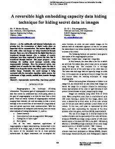
Fig. 5. Test images of 512 and bridge, and Grass.

2 512 2 8 bits. In the upper row and from left to right: Man, Baboon, and Girl. In the lower row and from left to right: Aerial, Stream

the basic embedding diagram and does not include the storage place exchange operation. Data extraction is implemented in the exactly reverse steps of data encoding. Before performing data extraction, we get back and from the LSBs of the first image pixels beginning from the upper left corner of the image. According to the structure of , we extract Flag Bit, , , and End Position in sequence. Then, according to the header file of JBIG file, we further get the length of . Afterwards, we perform JBIG decompression to resume . Relying on the embedding information of and , we scan the test image from the last embedded pixel (i.e., End Position) in the reverse raster scanning manner. . Based on , We perform (1) and get back from we first judge whether the current pixel is embedded or shifted and , and then, by using the combined information of , take the reverse operation by using (8), (9), (10), or (11). The original image is losslessly resumed as soon as the embedded secret message is completely extracted. III. EXPERIMENT AND DISCUSSION The proposed algorithm has been tested on different types of images. The six test images downloaded from the database2 are shown in Fig. 5. The experimental results of these test images are shown in Figs. 6 and 7. We compare our method with Tian’s DE method in [8], Kamstra et al.’s Extended DE method in [10], and Thodi et al.’s P2 method in [21]. Thodi et al. presented five versions of their algorithm, among which the prediction-error-expansion-based P2 method is one of the best. We evaluate the performance of these four algorithms by using the embedding capacity versus compressed (overflow) location map length curve and the embedding capacity versus image quality curve. For common images like Man, the histogram is sharp and narrow. Fig. 6(a) shows that P2’s compressed overflow location map has a constant length at different embedding rates, and the compressibility of the overflow location map is high. Different 2http://sipi.usc.edu/database/

from P2, our compressed overflow location map has changing lengths for different payloads. Our overflow location map has even higher compressibility though the advantage is not large. Fig. 6(b) shows that both P2 and our method have very good performance, but our method is slightly better than P2 in PSNR (peak signal-to-noise-ratio) values under the same payload. The location map of Tian’s DE method has very poor compressibility. When the payload is small, the compressed location map consumes far more embedding space than the payload. This is because Tian’s method lacks capacity control capability. As the payload becomes larger, the compressibility of Tian’s location map improves. The zigzag shape of DE method’s embedding capacity versus compressed location map length curve results from the combined effect of multi-layer embedding and the size of the difference image. The curve’s valley indicates that the compressibility of the location map reaches the highest when all expandable differences are used in the difference image. It can be seen that DE method has similar embedding capacity versus compressed location map length curves for all the six test images, and the major differences of these curves are in valleys and peaks. The advantage of our method over DE method is obvious. Fig. 6(b) shows that the largest PSNR difference between our curve and DE method’s is about 9 dB. Although the location map of Extended DE method has high compressibility, it is essentially different from the other three maps. This map is derived from the sorting list that is based on the characteristics of the low-pass image. Basically, this sorting list can not guarantee to give priority to small differences. As mentioned in [10], locations at the beginning of the sorting list are more likely to be expandable than locations that occur more toward the end. This statement implies that Extended DE method performs well under small payloads. For DE, P2 and our methods, high compressibility usually corresponds to good algorithm performance. However, the high compressibility of Extended DE method’s location map is mainly due to the smoothness of the low-pass image. As shown in Fig. 6(b), Extended DE method has good performance at low embedding rates, but its performance degrades quickly as the embedding rate increases. Specifically,



257

Fig. 6. Performance comparison on test images Man, Baboon, and Girl. We compare our method with Thodi et al.’s P2 method, Tian’s DE method, and Kamstra et al.’s Extended DE method. We give the embedding capacity versus compressed (overflow) location map length curve in the left column and the embedding capacity versus image quality curve in the right column.

from 0.5 bpp (bits per pixel), there is no much performance difference between Extended DE method and DE method. For texture images like Baboon, the histogram is flat. Fig. 6(c) shows that P2 has a much larger compressed overflow location map than our method. When the embedding rate is less than 0.7 bpp, P2’s compressed overflow location map is bits longer than ours. This result indicates that about 2 our method has the strong capacity control capability and our

payload-dependent overflow location map is highly compression-efficient. Only when the embedding rate is greater than 0.8 bpp, the length of our compressed overflow location map increases apparently. The increase in length accelerates from 0.9 bpp. This is because most of the expandable predicted errors are used for large payloads. Fig. 6(d) exhibits the advantage of our method over P2 and DE method. The largest PSNR differences between our curve and these two curves are about 7


258


Fig. 7. Performance comparison on test images Aerial, Stream and bridge, and Grass. We compare our method with Thodi et al.’s P2 method, Tian’s DE method, and Kamstra et al.’s Extended DE method. We give the embedding capacity versus compressed (overflow) location map length curve in the left column and the embedding capacity versus image quality curve in the right column.

dB and 15 dB, respectively. These results happen at 0.05 bpp. The smaller the payload, the larger the PSNR difference. As for Extended DE method, the length of its compressed location map increases rapidly at large embedding rates. Apparently, the smoothness of the low-pass image is not the only factor affecting the compressibility of the location map. Actually, Kamstra et al. used the same rule as Tian and Thodi et al. did when selecting expandable locations. As more locations are

selected for large payloads, more unexpandable locations are included in their sorting list. Thus, the location map derived from the sorting list has poorer compressibility. Since Kamstra et al.’s location map is a payload-dependent one, the problem of inefficient compression only becomes more serious as the payload increases. The reader is referred to [10] for more detailed information. Fig. 6(d) shows that our method is still better than Extended DE method, especially at medium embedding rates.



For high-tone images like Girl, the histogram is sharp and narrow, but P2 can not maintain its good performance. Fig. 6(e) shows that P2 has a compressed overflow location map with a very large size, about 4 10 bits. It indicates that Thodi et al.’s method is very sensitive to high-tone images. On the contrary, our overflow location map has good compressibility at low embedding rates. The length of our compressed overflow location map only increases as the payload increases. Fig. 6(f) shows that our method is apparently superior to P2 at low- and medium-embedding rates. P2’s PSNR values are even close to those of DE method from 0.1–0.3 bpp. The performance difference between our method and P2 dwindles as the payload increases. The length of compressed location map of Extended DE method increases quickly with the increase of the payload, so that Extended DE method only performs well at low embedding rates. Our method often performs much better than Extended DE method. Aerospace image Aerial has large flat regions, some of which are bright. Its histogram is sharp, but not as sharp as that of Man. Fig. 7(a) shows that the four curves often can not perform as well as their counterparts do in Fig. 6(a). Therefore, the four curves in Fig. 7(b) look like their counterparts in Fig. 6(b), but the performance of the former is often not as good as that of the latter. In particular, due to flat bright image regions, P2 faces the problem similar to that on Girl. Therefore, P2 has greater performance degradation than our method. The performance of Extended DE method also degrades more rapidly. When the embedding rate is less than 0.1 bpp, Extended DE method is even better than our method; but it performs almost as DE method does when the embedding rate is greater than 0.5 bpp. There are some images with partial textures and uneven brightness, for example, Stream and bridge. P2 faces two challenges. First, the histogram is not sharp but very ragged. Second, the image is very bright in some regions but very dark in others. Both of them have negative impact on the compressibility of P2’s overflow location map, and thus, degrade its performance. Fig. 7(c) shows that the length of our compressed overflow location map increases slowly. Fig. 7(d) demonstrates that our method outperforms the other three, and the performance difference is larger when the embedding rate is less than 0.2 bpp. Finally, we give an extreme example to further show how our method works. Grass is an image with strong textures and uneven brightness. Its histogram is much flatter and wider. Fig. 7(e) exhibits that the length of our compressed overflow location map increases very slowly when the embedding rate is less than 0.5 bpp. On the contrary, the other three methods perform poorly. The length of P2’s compressed overflow location map is about 4.5 10 bits. DE method has the embedding capacity versus compressed location map length curve with the poorest behavior among the six test images. The valley is not low and the peak is very high. As for Extended DE method, the length of its compressed location map increases rapidly from very small embedding rates. Fig. 7(f) demonstrates that our embedding capacity versus image quality curve is far above the other three curves at low- and medium-embedding rates.

259

Before finishing this section, we make a brief discussion on computational complexity of our proposed algorithm. Our simulation is carried out on a Pentium-4 3.44 GHz PC with 1G RAM. Our algorithm is implemented in Visual C 6.0. For image Man, the embedding process takes about 0.125 sec at 0.1 bpp and 0.985 sec at 0.99 bpp. The corresponding detection process takes about 0.047 sec and 0.078 sec, respectively. For different images and at different embedding rates, the consuming time would change a little. IV. CONCLUSION In this paper, we have investigated the problem of the overflow location map, which is an important issue in DE-based reversible data hiding. In order to increase embedding capacity, we improve the compressibility of the overflow location map by designing a new embedding scheme. Our overflow location map depends on the payload. Unlike other (overflow) location maps, it contains two types of overflow locations: one from embedding and the other from shifting. Since the constraint on shifting is looser than that on embedding, it results in fewer overflow locations. Therefore, our overflow location map matrix is often sparser than other current ones. This feature makes our overflow location map have higher compressibility. Our interleaving histogram shifting scheme also enhances capacity control capability, and thus, benefits image quality. Compared with other reversible data hiding methods in literature, the proposed algorithm often has better resilience to different images and larger embedding capacity under the same image quality. ACKNOWLEDGMENT The authors would like to thank the Associate Editor Prof. M. Barni and the anonymous reviewers for their valuable comments and suggestions that have helped us improve the quality and clarity of the paper. REFERENCES [1] C. W. Honsinger, P. Jones, M. Rabbani, and J. C. Stoffel, “Lossless recovery of an original image containing embedded data,” U.S. Patent 6 278 791, Aug. 21, 2001. [2] J. Fridrich, M. Goljan, and R. Du, “Lossless data embedding—New paradigm in digital watermarking,” EURASIP J. Appl. Signal Process., vol. 2002, no. 2, pp. 185–196, Feb. 2002. [3] R. Li, O. C. Au, C. Yuk, S.-K. Yip, and T.-W. Cha, “Enhanced image trans-coding using reversible data hiding,” in Proc. IEEE Int. Symp. Circuits Syst., May 2007, pp. 1273–1276. [4] Z. Ni, Y. Q. Shi, N. Ansari, and W. Su, “Reversible data hiding,” IEEE Trans. Circuits Syst. Video Technol., vol. 16, no. 3, pp. 354–362, Mar. 2006. [5] C. D. Vleeschouwer, J.-F. Delaigle, and B. Macq, “Circular interpretation of bijective transformations in lossless watermarking for media asset management,” IEEE Trans. Multimedia, vol. 5, no. 1, pp. 97–105, Mar. 2003. [6] J. Fridrich, M. Goljan, and D. Rui, “Invertible authentication,” in Proc. SPIE 2001, Security and Watermarking of Multimedia Contents III, P. W. Wong and E. J. Delp, Eds., vol. 4314, pp. 197–208. [7] M. U. Celik, G. Sharma, A. M. Tekalp, and E. Saber, “Lossless generalized-LSB data embedding,” IEEE Trans. Image Process., vol. 12, no. 2, pp. 157–160, Feb. 2005. [8] J. Tian, “Reversible data embedding using a difference expansion,” IEEE Trans. Circuits Syst. Video Technol., vol. 13, no. 8, pp. 890–896, Aug. 2003.


260


[9] A. M. Alattar, “Reversible watermark using the difference expansion of a generalized integer transform,” IEEE Trans. Image Process., vol. 13, no. 8, pp. 1147–1156, Aug. 2004. [10] L. Kamstra and H. J. A. M. Heijmans, “Reversible data embedding into images using wavelet techniques and sorting,” IEEE Trans. Image Process., vol. 14, no. 12, pp. 2082–2090, Dec. 2005. [11] D. M. Thodi and J. J. Rodriguez, “Prediction-error based reversible watermarking,” in Proc. IEEE Int. Conf. Image Process., Oct. 2004, vol. 3, pp. 1549–1552. [12] D. Coltuc and J. M. Chassery, “Very fast watermarking by reversible contrast mapping,” IEEE Signal Process. Lett., vol. 14, no. 4, pp. 255–258, Apr. 2007. [13] S. Lee, C. D. Yoo, and T. Kalker, “Reversible image watermarking based on integer-to-integer wavelet transform,” IEEE Trans. Inf. Forensics Security, vol. 2, no. 3, pp. 321–330, Sep. 2007. [14] T. Kalker and F. M. J. Willems, “Capacity bounds and constructions for reversible data-hiding,” in Proc. 14th Int. Conf. Digital Signal Process., Jul. 2002, vol. 1, pp. 71–76. [15] C.-T. Li , “Reversible watermarking scheme with image-independent embedding capacity,” Proc. IEE Vis. Image Signal Process., vol. 152, no. 6, pp. 779–786, 2005. [16] Z.-M. Lu, H. Luo, and J.-S. Pan, “Reversible watermarking for error diffused halftone images using statistical features,” in Proc. Int. Workshop Digital Watermarking, Nov. 2006, vol. LNCS 4283, pp. 71–81. [17] M. Fujiyoshi, S. Sato, H. L. Jin, and H. Kiya, “A location-map free reversible data hiding method using block-based single parameter,” in Proc. IEEE Int. Conf. Image Process., Sep. 2007, vol. 3, pp. 257–260. [18] C. C. Chang, W. L. Tai, and C. C. Lin, “A reversible data hiding scheme based on side match vector quantization,” IEEE Trans. Circuits Syst. Video Technol., vol. 16, no. 10, pp. 1301–1308, Oct. 2006. [19] X. T. Wang, C. Y. Shao, X. G. Xu, and X. M. Niu, “Reversible datahiding scheme for 2-D vector maps based on difference expansion,” IEEE Trans. Inf. Forensics Security, vol. 2, no. 3, pp. 311–320, Sep. 2007. [20] Y. Hu and B. Jeon, “Reversible visible watermarking and lossless recovery of original images,” IEEE Trans. Circuits Syst. Video Technol., vol. 16, no. 11, pp. 1423–1429, Nov. 2006. [21] D. M. Thodi and J. J. Rodriguez, “Expansion embedding techniques for reversible watermarking,” IEEE Trans. Image Process., vol. 16, no. 3, pp. 721–730, Mar. 2007.

Computer Engineering, Sung Kyun Kwan University, Korea. Since 2006, he has been visiting in the Department of Computer Science, Korea Advanced Institute of Science and Technology (KAIST), Daejeon, Korea, as a Visiting Professor. His research interests include information security, digital forensics, and image signal processing.

Heung-Kyu Lee received the B.S. degree in electronics engineering from the Seoul National University, Seoul, Korea, in 1978, and the M.S. and Ph.D. degrees in computer science from the Korea Advanced Institute of Science and Technology (KAIST), Daejeon, Korea, in 1981, and 1984, respectively. Since 1986, he has been a professor of the Department of Computer Science, KAIST, Korea. He is an author/coauthor of more than 100 international journal and conference papers. Dr. Lee is a reviewer for many international journals, including Journal of Electronic Imaging, Real-Time Imaging, IEEE TRANSACTIONS ON CIRCUITS AND SYSTEMS FOR VIDEO TECHNOLOGY, etc. He was also a program chairman of many international conferences, including the International Workshop on Digital Watermarking (IWDW) in 2004, IEEE International Conference on Real-Time Systems and Applications, etc. Since 2006, he has been a General Director of Center of Fusion Technology for Security (CFTS). His major interests are information hiding and multimedia forensics.

Jianwei Li received the B.E. degree from Xi’an University of Technology, Xi’an, China, in 2005. He is currently pursuing the M.S. degree in pattern recognition and intelligent systems in the College of Automation Science and Engineering, South China University of Technology, Guangzhou, China. His research interests include digital image processing, data hiding and pattern recognition.

Yongjian Hu received the Ph.D. degree from South China University of Technology, Guangzhou, China, in 2002. He is a Professor of the School of Electronic and Information Engineering, South China University of Technology. During 2000 to 2004, he visited the Department of Computer Science, City University of Hong Kong four times as a Research Assistant, Senior Research Associate, and Research Fellow, respectively. From 2005 to 2006, he worked as a Research Professor in the School of Electrical and
