In many real-life cases, domains are not available, and have to be acquired or .... Some CLP systems have an incomplete consistency check, thus the check may.
DEALING WITH INCOMPLETE KNOWLEDGE ON CLP(F D) VARIABLE DOMAINS MARCO GAVANELLI, EVELINA LAMMA, PAOLA MELLO, AND MICHELA MILANO Abstract. Constraint Logic Programming languages on Finite Domains, CLP(F D), provide a declarative framework for Artificial Intelligence problems. However, in many real life cases, domains are not known and must be acquired or computed. In systems that interact with the outer world, domain elements synthesize information on the environment, they are not all known at the beginning of the computation, and must be retrieved through an expensive acquisition process. In this paper, we extend the CLP(F D) language by combining it with a new sort (called Incrementally specified Sets, I-Set). In the resulting language, CLP(F D+ I-Set), FD variables can be defined on partially or fully unknown domains (I-Set). Domains can be linked each other through relations, and constraints can be imposed on them. We describe a propagation algorithm (called Known Arc Consistency, KAC) based on known domain elements, and theoretically compare it with arc-consistency. The language can be implemented on top of different CLP systems, thus letting the user exploit different possible semantics for domains (e.g., lists, sets or streams). We state the specifications that the employed system should provide, and we show that two different CLP systems (Conjunto and {log}) can be effectively used. We provide motivating examples and describe promising applications.
1. Introduction The Constraint Satisfaction Problem (CSP) [26] is a powerful framework for dealing with many problems in Artificial Intelligence. A CSP consists of a set of variables that range over some given domains, and are subject to a set of constraints. Constraints provide a natural way to formalize problems in a declarative fashion, and are embedded in Constraint Logic Programming (CLP) languages [23]. Constraint Logic Programming is a class of declarative programming languages, widely used both in research and in industrial applications, that enables the user to separate the problem description from the resolution algorithm. “Constraint programming represents one of the closest approaches computer science has yet made to the Holy Grail of programming: the user states the problem, the computer solves it.” [17]. A natural mapping of CSP can be given in terms of Constraint Logic Programming over Finite Domains, CLP(F D) [13]. In CLP(F D) programs, variables range over finite domains, and are constrained each other. Constraint propagation algorithms, like Arc-Consistency [26] and its evolutions, are often embedded in CLP(F D) solvers; the key idea is to remove domain values that cannot be part of a solution in order to prune the search space. CLP(F D) deals with constraint satisfaction problems in an elegant, declarative fashion, and could be considered as the language extension of the CSP framework. 1
However, in a CSP all data about the problem is needed at the beginning of the computation. In particular, domains have to be fully known: if some domain elements are not known, the solving process cannot start. A possible, but inefficient approach suggests to build a CSP containing only the available information and try to solve it; if a solution cannot be found, more information about domain values must be retrieved, and a new CSP must be constructed and solved from scratch. This limit is also inherited by CLP(F D): before constraint propagation can start, domains need to be defined. If the user does not provide domains, many systems will associate to variables some default domain (e.g., {−M axInt, . . . , +M axInt}) when the domain is the integer set; unlikely, this approach is applicable only to subsets of the integers, not to all the possible Finite Domains. In many real-life cases, domains are not available, and have to be acquired or computed. Often, constraints over them are known, but we do not know all their elements at the beginning of the computation. Suppose that domains are unknown but we know they are linked by a set of given relations; for instance, we could have three variables A, B, C that range on domains, respectively DA , DB and DC , that are subject to some constraints, e.g, DA ⊆ DB and DC ∩ DA = ∅. If domain values are provided by a different system, they must be derived before the CSP solving process starts. In other words, we have a strictly sequential computation: first a system yields the domains, then a CSP is constructed, and finally solved. This process is not acceptable in many problem instances. In most recognition tasks, for example, information comes from sensors in the form of signals, and has to be synthesized into symbols in order to be considered by the CSP model. Since signals and symbols are different in nature, this extraction and translation process is usually very time-consuming. Performing a whole computation that provides domains even if only some elements will be useful in CSP resolution can be a significant waste of time. A more efficient method would exploit the imposed constraints to prune the search space even on the computation providing domain values. An effective solution to this issue is the Interactive CSP (ICSP) model [8]. In this model, domains need not to be ground (i.e., fully known), their values are acquired or computed during the solution process only when needed, and then inserted into domains. The ICSP model has been successfully applied to visual recognition tasks [9] and planning [3]. Experiments on randomly-generated problems [10] show that in many instances, ICSP solving algorithms can avoid domain element acquisition steps, achieving good performance in problems where information is partially specified. In this paper, we propose a CLP language that fits with and generalizes the ICSP model. As CLP(F D) deals with CSPs, our language is aimed at solving ICSPs, and exploits ICSP algorithms in the propagation engine. In particular, we provide a CLP language that: • extends CLP(F D) to deal with incomplete knowledge on domains; • lets the user handle domains as first-class objects; • provides primitives for the interaction between the CLP(F D) solver and an acquisition system using domains as communication channels. In the proposed language, domains are Incrementally specified Sets, or I-Sets. We consider a CLP language combining two sorts: the Finite Domain (F D) sort and 2
the I-Set sort, that defines the domains of the F D variables. In this setting, constraints can be imposed on both F D variables, thus pruning the search space, and I-Set variables representing domains, thus providing information useful to synthesize domain elements. Intuitively, we want to enable the definition of domains as communication channels, and constraints over them as filters that remove inconsistent elements from the information flow possibly guiding knowledge acquisition. Communication channels will bring information from a domain element generator to a constraint solver. Constraints are exploited in two ways: (i) they are posted as requests to the domain element generator and (ii) are used as filters on domains. They are imposed on domains, thus they consider domains as first-class objects. We propose a propagation algorithm with lazy domain evaluation, in order to exploit the known information before requesting other information. The same propagation algorithm used for propagation in this language could be used in a wider framework. Besides the interaction between the F D sort and a provider of domain values, through I-Sets, the same algorithms could be used in conjunction with other CLP languages. For this reason, we generalize the framework to exploit other CLP(PF D ) (the powerset of F D) systems, such as Conjunto [18] or {log} [14]. We also define which features CLP(F D + PF D ) requires from the employed CLP(PF D ) system. The rest of the paper is organized as follows. In section 2 we provide the preliminaries and basic notation. In Section 3, we give the syntax and the declarative semantics of the proposed language. In Section 4, we show the operational semantics of the F D sort and the I-Set sort, we describe propagation of constraints that link the two sorts and we provide some examples. Section 5 gives some implementation details. In Section 6 we describe how our language can be generalized to employ other semantics for domains. Section 7 cites related work and promising applications. Conclusions and future work follow.
2. Preliminaries Throughout the paper we assume the reader to be familiar with the general principles and notation of logic programming languages. As usual in logic programming, uppercase letters are used for variables. The domain of a variable X will be indicated with DX . When considering a variable with an index, Xi , we will sometimes call Di its domain, instead of DXi . Constraint Logic Programming (CLP) [21] is a class of declarative languages. Each CLP language can be seen as an instance of a general CLP(X ) scheme where each instance can be specified by instantiating the parameter X [22]. The parameter X represents a 4-tuple (Σ, D, L, T ) where Σ is a signature, D is a Σ-structure, L is a class of Σ-formulas and T is a first-order Σ-theory. Let D be the set of elements of D. The signature Σ represents the predefined predicates and function symbols, D is the domain structure, L is a class of constraints which can be expressed in the domain and T is the axiomatization of some properties of D. Each CLP language can be defined by specifying all the 4-tuple components. Each CLP system is determined by the constraint domain (D, L) and by the operational semantics. 3
The general semantics of CLP languages was given by Jaffar and Maher [22]; we report it for the sake of completeness. 2.1. Semantics of CLP. Concerning the declarative semantics of a CLP(X ) program, we can view each rule A :- L1 , . . . , Ln . as representing the logical universally quantified formula A ← L1 ∧ · · · ∧ Ln The program is understood to represent the conjunction of its rules. The logical semantics of a CLP(X ) program is the theory obtained by adding the theory of the constraint domain C = (D, L) to the rules of the program. The operational semantics of a language that is instance of the CLP(X ) general scheme can be given in terms of a transition system [22]. States are represented by triples hA, C, Si where A is a multiset of atoms and constraints (representing the current goal), and (C, S) is called the constraint store. In particular, C is the constraint store of active constraints, i.e., constraints that are awake, and S is the constraint store of passive constraints, i.e., constraints that are asleep. The failure of the system is represented by a state called fail. The transition system is very general, but can be parameterized by defining the set of active and passive constraints, plus a predicate consistent and a function infer, both tailored on the particular domain. The first transition is denoted by →r where r stands for resolution: hA ∪ a, C, Si →r hA ∪ B, C, S ∪ (a = h)i if a is an atom selected by the computation rule, and h ← B is a rule of the program P , renamed to new variables, and h and a have the same predicate symbol. It is worth noting that in this transition we do not need to use a substitution because the term a = h is stored in the constraint store S, and will be processed in the following steps. Unification itself, in fact, can be seen as a constraint solving process. Transition →r can lead to a failure if h and a have not the same predicate symbol for each clause of the program P: hA ∪ a, C, Si →r f ail. The second transition is denoted by →c , where c stands for constraint, and introduces constraints into the constraint store: hA ∪ c, C, Si →c hA, C, S ∪ ci where c is a constraint selected by the computation rule. The third transition rule, denoted by →i where i stands for infer, infers new active constraints and modifies (generally simplifies) the passive constraints starting from the current constraint store (C, S) with the function (C 0 , S 0 ) = infer(C, S) hA, C, Si →i hA, C 0 , S 0 i. The last transition rule, denoted by →s , where s stands for satisfiability, tests whether the active constraints are consistent with the predicate consistent(C). Some CLP systems have an incomplete consistency check, thus the check may 4
succeed even if no solution is possible. In complete constraint systems, the predicate ˜ (where ∃C ˜ denotes the existential closure of C). consistent(C) holds iff D |= ∃C Therefore, if consistent(C) the transition is hA, C, Si →s hA, C, Si otherwise, the transition is hA, C, Si →s f ail. A derivation for a goal is a sequence of transitions hA1 , C1 , S1 i → · · · → hAi , Ci , Si i → . . . where →s are one of the above-mentioned transitions, the starting state is hGoal, ∅, ∅i and the final state is a state which cannot be rewritten further. This final state is successful if has the form h∅, C, Si, otherwise it is failed. 2.1.1. Operational semantics of CLP(F D). In particular, the operational semantics of CLP(F D) can be given by instantiating the function infer and the predicate consistent. The function infer, for most CLP(F D) systems, applies constraint propagation. Constraint propagation removes from variable domains those values which are proved infeasible. The basic constraint propagation embedded in finite domain solvers is based on consistency techniques, which were originally developed to solve Constraint Satisfaction Problems. Definition 1. A Constraint Satisfaction Problem (CSP) is a triple hX, D, Ci where X = {X1 , . . . , Xn } is a set of variables, ranging on some finite domains D = {D1 , . . . , Dn } and subject to a set of constraints C. A solution of a CSP is an assignment of values taken from the domains to the corresponding variables such that all the constraints are satisfied. Without losing generality, we can focus only on binary CSPs, i.e., CSPs that contain only unary and binary constraints. We now recall two consistency techniques [26]: Definition 2. A unary constraint cA on the variable A is Node Consistent iff for each value v belonging to the domain DA , cA (v) is true. Definition 3. A constraint cA,B on variables A and B is Arc Consistent iff for any value x belonging to DA , a value y belonging to DB exists such that the constraint cA,B (x, y) holds. The definition of Arc Consistency can then be extended to a whole CSP. Definition 4. A CSP is Arc Consistent if all the unary constraints are Node Consistent and the binary constraints are Arc Consistent. Arc Consistency can be achieved by removing domain elements inconsistent with constraints. Given a CSP that is not Arc Consistent, propagation yields an equivalent CSP which is Arc Consistent. Intuitively, one would like to get to a network where variables’ domains are smaller, but no solution is removed. More precisely, let us define the concept of subdomain [30]: Definition 5. Given a CSP=hX, D, Ci where D = (D1 , . . . , Dn ) is the domain of the CSP, we say that D0 = (D10 , . . . , Dn0 ) is a subdomain of D iff ∀ni=1 Di0 ⊆ Di . 5
procedure AC Q ← {c(Xi , Xj )}; while not empty(Q) select and delete one constraint c(Xk , Xm ) from Q; if REVISE(c(X k , Xm )) then S Q ← {c(Xi , Xk ) such that i 6= k ∧ i 6= m} EndIf; EndWhile; End KAC function REVISE(c(Xi , Xj )):bool; MODIFIED ← false; for each vi ∈ Di do if there is no vj ∈ Dj such that (vi , vj ) ∈ c(Xi , Xj ) then MODIFIED ← true; delete vi from Di ; EndIf; EndFor; return MODIFIED; End REVISE Figure 1. AC-3: an algorithm for Arc Consistency enforcing In general, given a CSP which is not Arc Consistent, there are many Arc Consistent subdomains; an algorithm achieving Arc Consistency computes the maximal Arc Consistent subdomain. Many algorithms have been proposed to enforce Arc Consistency, the most widely used in CLP(F D) languages is AC-3 [26], reported in Figure 1. Concerning the predicate consistent, in CLP(F D) solvers, inconsistency is detected when the domain of a variable is shown to be empty. Since finite domain solvers are not complete, the consistency check can be successful even if the problem is infeasible. Therefore, search is needed when the propagation reaches a fix-point to guess the value for a given variable and restart the constraint propagation process. 3. CLP(F D + I-Set): Syntax and Declarative Semantics The language we propose extends CLP on finite domains, CLP(F D), with incomplete knowledge on variable domains. This language has shown to be an effective tool for representing and solving many real life applications, modelled as Constraint Satisfaction and Optimization Problems. In a CLP(F D) program, the user has to specify variables, the corresponding finite domains, constraints among them, and a search strategy. In particular, in CLP(F D) the user has to completely specify all values belonging to the domain of each variable. The extended language we propose lets the user work with unbound domains, interactively acquire new information, and impose constraints on domains. The proposed language is a two-sorted CLP language, where the sorts are the classical FD sort on finite domains and a sort based on sets. 6
We first define constraints and operations on the two sorts, then we combine them so as to enable the second to represent the domains for the variables in the first. 3.1. The F D sort. The F D sort is based on a finite set DF D , that contains all the possible values that the variables may assume. The signature ΣF D , besides the elements in the DF D set, contains the binary predicate :: plus operations and constraints defined on the particular instance. The symbol :: can only have ground terms as the second argument, and is interpreted as a unary constraint with the following meaning: given a set of ground elements {v1 , ...., vn } and a variable X, the constraint X :: {v1 , ...., vn } holds if and only if X = v1 ∨ X = v2 ∨ · · · ∨ X = vn . The constraints LF D are generated by the primitive constraints restricted so that any variable appearing in a constraint is subject to a unary :: constraint. An often used instance of the F D sort is a subset of the integer sort (let us call it F DZ ). In this case, the set of elements of the domain is DF DZ = Z, and the signature ΣF DZ also contains the symbols { Y. 3.4. Examples. Let us see some examples of programs that can be naturally given in the CLP(F D+I-Set) language. 9
3.4.1. Map Colouring. To get the flavor of the power of the defined language, let us consider a classical CSP example: the map-colouring problem. The problem consists in finding a colour for each country in a map, such that neighbouring countries have different colours. Variables represent the countries, the domains contain the available colours and constraints state that neighbouring countries have different colours. For example: F rance, Italy, Germany, Switzerland :: {red, green, blue} with the constraints: F rance 6= Italy, F rance 6= Germany, F rance 6= Switzerland, Italy 6= Switzerland, Germany 6= Switzerland In this example the palette is known (i.e., the domain {red, green, blue}); the problem can be extended to deal with incomplete knowledge about domains. Suppose that the palette is not available at the beginning of the computation, but it is incrementally specified during constraint processing. In our language, a variable Palette will represent the set of available colours: F rance, Italy, Germany, Switzerland :: P alette In other situations, different countries may take values from different sets, possibly related through constraints. Suppose, as an example, that three different robots will paint a map, in different areas. The colours themselves will be provided by a system that generates color(R, G, B) triplets, according to some rules. The robot in the middle can access the colors in the palette of the other two robots. So, the constraint between the different palettes can be stated as: union(P alette1 , P alette3 , P alette2 ) we associate the countries painted by one robot with its available palette: F rance, Italy :: P alette1 Germany :: P alette2 , Switzerland :: P alette3 In our language, the user can impose the usual constraints of CLP(SET) languages when defining domains, and nonetheless, efficiently combine the solver on sets with the constraint propagation of the F D solver, as will be shown later. In particular, we aim at minimizing the acquisition of domain elements. 3.4.2. A vision system. Let us consider again the example of the vision system. As noted earlier, the constraint solver is not isolated, but needs to communicate with external components that provide the image features. The segmentation process can be very time consuming, because of the difference in nature between the image (which is a type of signal) and the segments (that represent symbolic information). Thus, if the goal is finding if a rectangle is present in the scene, there is no point in extracting all the possible segments even if the first four segments already form a rectangle. An efficient system must minimize the number of extracted primitives. In our framework, we can state that the variables range over the set of segments in the image, which is unknown at the beginning of the computation: X1 , X2 , X3 , X4 :: Segments 10
Then, each time a segment si is retrieved, it will be inserted in the I-Set Segments over which the F D variables range. In 3D recognition, the problem is even harder [9]. Various types of features are often employed, so we might have variables ranging on surface patches, others ranging on segments, others on angles. In our language, this situation can be easily specified: S1 , S2 , . . . , Si :: Segments P1 , P2 , . . . , Pj :: Surfaces A1 , A2 , . . . , Ak :: Angles In this way, different acquisition modules can be exploited at the same time, providing in parallel different classes of information. It is worth noting that even in human vision there are different brain parts that carry on recognition of different classes of features (e.g., horizontal and vertical lines). Moreover, from a certain viewpoint, a surface may appear as a segment; in this case we can state that some variable can range on the union of the two sets: Sx :: D, union(Segments, Surfaces, D). If we have two cameras, we can exploit stereo-vision in order to infer distance information about the various objects. Of course, the two cameras will see only some objects in common, so a variable could range only on the intersection of the set of objects: S3D :: D3D , intersection(CameraL , CameraR , D3D ). 4. Operational Semantics The operational semantics of the proposed framework is defined by the propagation of constraints in the two sorts, plus the propagation of the constraint :: that links the sorts. 4.1. CLP(I-Set). Declaratively, the semantics of the I-Set sort is the same of a Set sort. Operationally, in order to achieve high efficiency, we avoid non-deterministic unification [14]. To this purpose, we restrict the language by forbidding non ground terms to enter as members of an I-Set. Thanks to this restriction, a most general unifier between two I-Sets can be easily computed in polynomial time. Let I1 and I2 be two I-Sets. In the most general case each of them can be partitioned into a known part, containing only ground elements, and an unknown part, which can be a variable or an empty I-Set; i.e., I1 ≡ K1 ∪ U1 and I2 ≡ K2 ∪ U2 . After unification between I1 and I2 , we want all the known elements to belong to the known part of both the domains and the unknown parts to be equal. So, I-Set parts vary as follows: U1 = (K2 \ K1 ) ∪ U10 U2 = (K1 \ K2 ) ∪ U20 where Ui0 and Uj0 are two new I-Set variables, representing the common unknown domain part, which are unified in their turn, i.e.: Ui0 = Uj0 For example, if I1 = {1, 2, 4, 8|U1 } and I2 = {1, 2, 3|U2 }, the unified set will be {1, 2, 3, 4, 8|U 0 }. This is equivalent to imposing that U1 = {3|U 0 } and U2 = {4, 8|U 0 }. 11
Constraints access an I-Set through the following low-level primitives (whose code is given in Fig. 3): • insert(S, E): inserts a ground element E in the I-Set S. If E was already inserted in S, insert does nothing. Otherwise, if S is open, this primitive adds E to S; if S is closed and E does not belong to S, then it fails. • get(S, E): unifies E with an element that was previously inserted in S. If no element in S can be unified to E and S is open, it suspends. If no element can be unified and S is closed, then it fails. • known(S, L): provides the list of known elements in S. • close(S): states that no more elements belong to the I-Set. These primitives will not generate repeated elements in an I-Set, even if they are allowed by the syntax. In the code in Figure 3, we use the syntax of ECLi P S e [20] for declaring that the goal get(S,E) should be delayed whenever S is a variable. insert(S,E) :- nonground(E), !, raise_exception. insert(S,E) :- var(S), !, S={E|_}. insert({},E) :- !, fail. insert({E|_},E) :- !, true. insert({_|T},E) :- insert(T,E). delay get(S,E) if nonvar(S). get({},_) :- !, fail. get({E|_},E) :- !. get({_|T},E) :- get(T,E). known(S,[]) :- var(S), !. known({},[]). known({E|T},[E|T1]) :- known(T,T1). close(S) :- var(S), !, S={}. close({}). close({_|T}) :- close(T).
Figure 3. Primitives All the other operations, and constraints in particular, are based on the primitive operations. All the constraints can propagate in polynomial time, since they only need to perform simple operations on ground lists. Whenever a constraint cannot propagate, it simply suspends. 4.2. Linking the two sorts: CLP(F D+ I-Set). As mentioned in Section 2.1, CLP(F D) systems use constraint propagation (mainly Arc Consistency and its extensions) as solver. In particular, constraint propagation removes inconsistent values from the domains of the F D variables (in the infer transition) and detects inconsistency (in the satisfiability transition) when a domain is empty. In our language, F D variables range on I-Sets; however, if an I-Set contains an element v, this element cannot be deleted by constraint propagation on F D variables. Therefore, we need to distinguish the concept of Definition Domain (i.e., the one represented by the corresponding I-Set) and of Current Domain (i.e., the one which is restricted by F D constraint propagation). • We will call Definition Domain an I-Set over which an F D variable ranges. For example, if X :: D, then D is X’s definition domain. The Definition 12
Domain is accessible at language level, thus, it can be defined intensionally by constraints. Its state can be modified exclusively by constraints imposed on it, never by constraints imposed on the Xi variable ranging on Di . The d Definition Domain of the variable X will be indicated with DX , its known d d part as KX and the unknown part with UX . • With Current Domain we will indicate a set of values that an F D variables could assume. It is a data structure hidden at the language level, that can be considered an extension of the concept of domain in usual CLP(F D) systems. In fact, values can be removed from it when proved inconsistent by constraint propagation, and if the domain is proved empty, predicate consistent will fail. In our framework, it also contains an unknown part. c , its known The current domain of a variable X will be indicated as DX c c part will be KX and the unknown part will be UX . The propagation of the :: constraint, that links the two sorts, is aimed essentially at communicating information from the I-Set sort to the F D sort. c d c is maintained true. DX ⊆ DX For each F D variable X, the basic property DX must synthesize all the knowledge provided by the definition domain; in particular, the known elements and the (eventual) emptiness of the unknown part. Also, all the elements in the known part of the definition domain should be also communicated to the F D sort, thus enter in the known part of the current domain in order to be exploited for propagation. Then, if they are inconsistent, they will be removed by subsequent propagation. Knowledge on the unknown domain part is important because we can exploit it for constraint propagation. In fact, a domain element v ∈ Ki can be removed by a binary constraint c(Xi , Xj ) only if we know that it is not supported by any element in the domain of Xj ; as any element could be supported by yet unknown elements, we cannot delete it if the domain of Xj is not fully known (i.e., not closed). 4.3. CLP(F D). As mentioned, in CLP(F D) domains are fully known. Thus propagation of constraints checks if each element has a support. Here we propose an extension of the concept of consistency for the partially known case, called known consistency. In this paper, we provide only the extension of node-consistency and arc-consistency; the extension to higher degrees of consistency is straightforward. Definition 6. A unary constraint c(Xi ) is known node-consistent iff ∀vi ∈ Kic , vi ∈ c(Xi ) Definition 7. A binary constraint c(Xi , Xj ) is known arc-consistent iff ∀vi ∈ Kic , ∃vj ∈ Kjc s.t. (vi , vj ) ∈ c(Xi , Xj ) Definition 8. A constraint network is known arc-consistent (KAC) iff all unary constraints are known node-consistent and all binary constraints are known arcconsistent. Known Arc Consistency shares some nice features with Arc Consistency (AC). The following lemma will be used to prove that a solver based on KAC detects inconsistency in the same instances as AC. Lemma 1. If a network of constraints is KAC, then the subset of known elements is an arc-consistent subdomain. 13
Proof. From definition 8, for each constraint c(Xi , Xj ) each known element in Dic has a support in Djc . ¤ As we mentioned earlier, enforcing arc-consistency means translating a given problem P into a different but equivalent problem P 0 in which the constraint network is arc-consistent. Many algorithms have been given [34] [26] [29] [19] [4] [5] for computing arc-consistency; the algorithms have different performance, but all detect inconsistency in the same problem instances (when a domain becomes empty). In the same way, there are many algorithms that translate a problem, P , into an equivalent problem P 0 , with different domains, such that the new problem P 0 is KAC. Proposition 1. Every algorithm achieving KAC (i.e., any algorithm that computes an equivalent problem that is KAC) and that ensures at least a known element in each variable domain is able to detect inconsistency in the same instances as an algorithm achieving AC. Proof. An algorithm achieving KAC computes an arc-consistent subdomain (lemma 1). Since each domain must contain at least one (known) element, then the obtained known subdomain is a not empty subset of the maximal arc-consistent subdomain. ¤ In other words, if an arc-consistent subdomain exists, then a maximal arcconsistent subdomain exists; so if KAC does not detect inconsistency, AC will not detect inconsistency either. The advantage in using KAC is that the check for known arc-consistency can be performed lazily, without full knowledge of all the elements in every domain. Operationally, achieving KAC has some similarities with achieving Lazy Arc Consistency (LAC) [30]. LAC is an algorithm that finds an arc-consistent subdomain (not necessarily a maximal one) and tries to avoid the check for consistency of all the elements in every domain. KAC looks for an arc-consistent subdomain as well, but it is aimed at avoiding unnecessary information retrieval, rather than unnecessary constraint checks. In order to achieve AC, algorithms need to remove elements that are proven to be inconsistent. In order to achieve KAC, algorithms need to delete elements and to promote elements, i.e., to move ideally some elements from the unknown part to the known part. In order to use KAC for propagation, a low-level predicate promote should be implemented, with the syntax: promote(V, I) where I is an I-Set and V is a variable. Intuitively, promote(V, I) should synthesize a new element V that belongs to the unknown part of the I-Set I, and which was not synthesized before. The predicate promote provides in V a ground term with the following declarative semantics: promote(V, I) ⇔ (V ∈ UI ∧ V ∈ / KI ) Elements can then be deleted if they are shown to be inconsistent. In figure 4 an algorithm for achieving KAC is shown, based on AC-3 as presented in Figure 1; we only need to change a few lines in function REVISE. Other algorithms could be employed as well. If all domains are fully known from the beginning of the 14
computation, then procedure KAC provides maximal subdomains, i.e., it computes AC. function REVISE KAC(c(Xi , Xj )):bool; MODIFIED ← false; for each vi ∈ Kic do if there is no vj ∈ Kjc such that (vi , vj ) ∈ c(Xi , Xj ) then FOUND ← SEARCH UNKNOWN(c(Xi , Xj ),vi ); if not FOUND then delete vi from Kic ; MODIFIED ← true; EndIf; EndIf; EndFor; return MODIFIED; End REVISE function SEARCH UNKNOWN(c(Xi , Xj ),vi ):bool; CONSISTENT ← false; EOA ← false; while not CONSISTENT and not EOA if promote(V, Dj ) then Uj = {V |Uj0 }; CONSISTENT ← (vi , V ) ∈ c(Xi , Xj ); else EOA ← true EndIf; EndWhile; End SEARCH UNKNOWN;
Figure 4. KAC propagation for FD constraints
4.4. Example: Numeric CSP. Let us see with a simple example, how a sample problem can be described and solved in CLP(F D+I-Set). With the given language, we can state in a natural way the following problem: :-X :: DX , Y :: DY , Z :: DZ , intersection(DX , DY , DZ ), Z > X. defining three variables, X, Y and Z, with constraints on them and their domains. KAC propagation can start even with domains fully unknown, i.e., when DX , DY and DZ are variables. Let us suppose that the elements are acquired through interaction with a user (i.e., the promote predicate is specialized for acquisition from a user) and the first element retrieved for X is 1. This element is inserted in the d d 0 domain of X, i.e., DX = {1|(DX ) }; since it is consistent with F D constraints, it is c c 0 = {1|(DX ) }. Then KAC propagation also inserted in the current domain, i.e., DX tries to find a support for this element in each domain of those variables linked by F D constraints; in our instance DZ . A value is requested for DZ and the user gives a value: 2 (Figure 5). This element is inserted into the domain of Z: d d 0 DZ = {2|(DZ ) }. The acquired element is also consistent with Z > X and a support exists for it in DX , thus it is inserted in the current domain of Z. Finally, the constraint imposed on domains can propagate, so element 2 has to be inserted in both the (definition and current) domains of Y and X, thus DYc = DYd = {2|DY0 } c d 00 and DX = DX = {1, 2|DX }. 15
c KAC propagation must now find a known support for element 2 in DX , so another request is performed. If the user replies that there is no further consistent element in the domain of Z, then 2 is removed from the current domain of X (because of the propagation of constraint Z > X, and since DZ has been closed. Value 2 will remain in the definition domain of X because the element semantically belongs to the domain even if no consistent solution can exist containing it. When KAC propagation reaches the quiescence, in each domain we know a support for each other known value. It is worth noting that KAC produces an arc-consistent subdomain. To produce a solution, a search step through a labeling procedure should be performed as in traditional CLP(FD). The labeling instantiates each variable Xi to a value v in its known domain part. The propagation is triggered at each step and reinforces KAC. On backtracking v is deleted from the current domain and KAC is again reinforced (eventually promoting new values in the known part).
5. Implementation Details In various significant real-world constraint problems, the expected result is an assignment of values to the F D variables; in our language domains should be incrementally specified, because the synthesis of domain values is expensive, and acquired only on-demand. This was the purpose of the ICSP framework [8]. For example, in the Vision System described in section 3.4.2, the user is mainly interested in the association of image parts with model parts, not in the I-Sets representing the domains. In these instances, the propagation algorithm can be specialized, in order to further reduce the number of acquired features and gain efficiency. From a language viewpoint the user can set a flag through a directive and use the specialized acquisition algorithm. In fact, domain values can be requested to the acquisition system by means of constraints, and they can be used to guide the extraction of consistent domain values. We reach what we call guided acquisition. Since not-yet-extracted domain values semantically belong to the unknown part of a domain, the constraints used for acquisition are imposed on the unknown domain parts. We call them Auxiliary Constraints. Auxiliary Constraints are imposed by F D constraints and can also help the propagation. :- X :: Dx, Z :: Dz, intersection(Dx,Dy,Dz), Z > X. List new values for X: {1|Dx0 }. List new values for Z: {2|Dz 0 }. List new values for Z: {}. Dx={1, 2 | }, Dy={2 | Dy’}, Dz={2 | Dz’} X::{1 | }, Y::{2 | }, Z::{2 | } delayed goals: intersection(Dx,Dy,Dz) Z>X yes.
Figure 5. Example of computation 16
For example, the propagation of a constraint c(Xi , Xj ) deletes inconsistent elements from the known domain part and imposes the auxiliary constraints cuj (Xi , Ujc ) and cui (Uic , Xj ) over unknown parts. A constraint like cuj (Xi , Ujc ) is a relation between an object and an I-Set of objects, linking every domain element with a subset of the second domain. For instance, a constraint X > 5, where X :: D and D = {1, 10|U }, produces the new current domain {10|U 0 }, with the imposed auxiliary constraint ∀v ∈ U 0 , v > 5. Definition 9. A constraint c(Xi , Xj ) defines two auxiliary constraints cui (Uic , Xj ) and cuj (Xi , Ujc ). cui (Uic , Xj ) (resp. cuj (Xi , Ujc )) is a subset of the cartesian product P(Dic ) × Djc (resp. Dic × P(Djc )) representing couples of compatible assignments of the subdomain Uic ⊆ Dic (resp. Ujc ⊆ Djc ) and the variable Xj ∈ Djc (resp. Xi ∈ Dic ). It is satisfied by a couple of assignments Uic = Si ⊆ Dic , Xj = vj (resp. Ujc = Sj ⊆ Djc , Xi = vi ) iff ∀vi ∈ Si (resp. ∀vj ∈ Sj ), (vi , vj ) ∈ c(Xi , Xj ) An auxiliary constraint can only be generated by another constraint (it is not accessible at the language level) and its purpose is twofold. First, it prohibits inconsistent elements from entering the current domain, i.e., whenever new information is available, it checks the synthesized elements before their insertion in the current domain. Second, it can be exploited to provide information on consistent elements, and to help the synthesis of consistent elements only. In fact, the predicate promote can be implemented to select only elements consistent with the auxiliary constraints. This possibility can provide a huge performance improvement, but it can be exploited only if we are not interested in computing definition domains, but only (consistent) current domains. In fact, the synthesis of elements guided by auxiliary constraints has an implicit influence on the I-Set computation: elements inconsistent with F D constraints will not be generated, even if they semantically belong to an I-Set. Stated otherwise, we may drop completeness in order to obtain a further speedup. This is acceptable in many real-life problems. The user could be interested in using our language for defining open domains, and not in the computation on the domains themselves. In some cases, the user does not even impose constraints on I-Sets. In our language, the user may define the acquisition strategy through the language directive: :- use auxiliary cst. which enables the acquisition guided by auxiliary constraints. For example, in a visual search problem [9], we have exploited auxiliary constraints by passing them (in the promotion of elements) to an acquisition module that extracts visual features (such as segments or surfaces) from an image. Auxiliary constraints have provided information to the extraction agent, and focused its attention on the most significant image parts. For example, the auxiliary constraint touchuj (si , Uj ) provides information about the searched features: we are looking for surfaces near surface si , so the segmentation system will only look for surfaces in the vicinity of si . We implemented our framework on the ECLi P S e [20] CLP system; the architecture of the implementation is depicted in Figure 6. F D constraints impose 17
link
CLP(FD) X
…
c
:: D X
c(X) Aux DdX
… CLP(℘FD) request message
values
World / Acquisition system
Figure 6. Architecture for guided acquisition auxiliary constraints. In current implementation, only unary auxiliary constraints are allowed, because we suppose that the acquisition system providing values taken from the outer world is able only to check unary constraints. If the acquisition agent is more powerful, the architecture can be simply extended. Auxiliary constraints are passed to the acquisition agent and can be exploited to provide possibly consistent values. Each retrieved value belongs semantically to the definition domain of the considered variable, thus it is inserted. Propagation of the :: constraint provides values from the definition domain to the current domain; this value passing is filtered by auxiliary constraints. Other elements can be deleted by constraints imposed on the F D side. 6. Generalization: CLP(F D+PF D ) The same interaction scheme used for binding the F D and the I-Set sorts may be used in more general cases. It could be used for binding F D with other sorts representing collections of objects taken from a Finite Domain. We call the general sort dealing with collection of values PF D because it is based on the powerset of F D. The PF D sort can be considered an extension of the I-Set sort because it shares the same declarative semantics, but allows for a wider syntax or for different operational semantics. {log} can be considered as an example of a CLP(PF D ) language; its declarative semantics is the same as for I-Sets, but the syntax also allows for finitely nested sets, and sets may contain non-ground terms. From a language viewpoint, we want the employed CLP(PF D ) language to provide the constraints given in Section 3.2. Other requirements come from the operational semantics and will be discussed in Section 6.1. Our framework can be implemented on top of different CLP languages, dealing with different domain formalizations, thus achieving different expressive power and efficiency levels. Besides I-Sets, we could build a two-sorted CLP system on top of a CLP dealing with lists [7] or sets [16, 18]. Of course, the obtained system inherits advantages and drawbacks from the host language. For example, sets are managed in a wide variety of ways, so, if we have a combinatorial problem and need a very efficient system, we can choose Conjunto [18], while if we need higher expressive power, we may prefer {log} [14]. 18
6.1. Operational Semantics, Generalization: PF D sort. We define properties and behaviours that the sort on domains should provide in order to be exploited in our framework. Then, we show that two utterly different systems (Conjunto and {log}) can give the requested functionalities. We could thus obtain some interesting variants: Lazy Conjunto, (i.e, using Known Arc-Consistency in Conjunto), or CLP(F D)+{log} (i.e., F D propagation in {log}). Since the scope of our computation is finding solutions to a CSP, we need to distinguish domain elements that can be fruitfully exploited in a CSP computation from elements that are not yet known. For this reason, the employed system should allow the partitioning of each domain Did into a known and an unknown part (respectively, Kid and Uid ), with the intended meaning that the known part contains all the ground elements, while the unknown part is the rest. The following properties should be provided by a CLP(PF D ) system to be included in the CLP(F D+PF D ) framework: Property 1. Partitioning domains into a known and an unknown part: for each domain Did , at every step of the computation, the set of (ground) elements that are proven to belong to the set can be distinguished. We call this set the known domain part Kid . The rest of the domain (i.e., the set UiD = Did \Kid ) is called the unknown domain part • In {log} domains are given by an arbitrary collection of Prolog terms; sets are built using the set constructor {.|.} plus the empty set ∅. For example, {1, p(2), Z, q(Y, 3)|K} is a valid set. {log} satisfies Property 1; the known part is the set of ground elements that are proven to belong to a set, in our example, {1, p(2)}. Also, each time a new element is proven to belong to the known part, we need to impose a constraint stating that the element must not belong to the new unknown part. For example, if we have a domain containing Di = {p(a, X), p(Y, b)} (thus Kid = ∅), and we prove that p(a, b) ∈ Did we have (Kid )0 = {p(a, b)} and (Uid )0 = {p(a, X), p(Y, b)}; we will have thus to impose an explicit constraint stating p(a, b) ∈ / (Uid )0 . • In Conjunto a set S is represented by two ground sets: a Least Upper Bound (LUB) and a Greatest Lower Bound (GLB), such that GLBS ⊆ S ⊆ LU BS . Conjunto satisfies Property 1 and the known part coincides with the GLB, as it contains all the elements that definitely belong to the set. The unknown domain part is simply given by the set difference Uid = Did \ Kid = LU B \ GLB, because it contains the elements that may belong to the set. In this case, the term unknown is not well-suited, because in Conjunto all the domain elements have to be known. We use it here to keep the same symbols of the rest of the paper. Property 2. Promotion of elements: It is possible to define a predicate promote which can select an element from the unknown domain part and synthesize or acquire enough information to let it enter the known domain part. The promote predicate can be implemented in a variety of ways, depending on the problem and on the PF D sort we are exploiting. In general, each computation that provides enough information about domain elements can be exploited in this predicate (i.e., each computation that synthesizes a ground element can be used to implement the promote predicate). In the I-Set sort, i.e., when domains can be seen as communication channels between subsystems, the promotion is a request 19
for a domain element to the value provider. For instance, it can be used for human interaction (the user declares the domain elements) or for acquisition of information from another component. Property 3. Test/Assertion of emptiness: the promote predicate has to provide a ‘null value’ information if there are no more elements in the unknown domain part to be promoted. In other words, promote must be a predicate reporting false if there are no more consistent values. This property is very important, as we need a way to test if the unknown part is empty, i.e., the I-Set representing the F D domain is closed. 7. Related work Many systems consider set objects, because sets have powerful description capabilities. In particular, some have been described as instances of the general CLP(X ) framework [23], like {log} [14, 15], CLPS [25], or Conjunto [18]. In {log} [14, 15], a set can be either the empty set ∅, or defined by a constructor with that, given a set S and an element e, returns the set composed of S ∪{e}. This language is very powerful, allowing sets and variables to belong to sets. However, the resulting unification algorithm is non-deterministic; in the worst case, it has an exponential time complexity. Conjunto [18] is a constraint logic programming language in which set variables can range on set domains. Each domain is represented by its greatest lower bound and its least upper bound. Each element in a set must be ground, sets are finite, and they cannot contain sets. These restrictions avoid the non-deterministic unification algorithm, and allow for good performance results. In an I-Set only ground elements are allowed; this allows high efficiency. If we allow non-ground elements to be in an I-Set, we obtain a more expressive framework, like {log}; thus if more expressive power is necessary, another instance of the CLP(F D+PF D ) framework, the CLP(F D)+{log} instance, can be used. Codognet and Diaz [6] described a method for compiling constraints in CLP(F D). In their language, clp(FD), there is only one primitive constraint X in R, used to implement all the other constraints. R represents a collection of objects and can also be a user function. Thus, in clp(FD) domains are managed as first-class objects; our framework can be fruitfully implemented in systems exploiting this idea. Sergot [32] proposes a framework to deal with interaction with the user in a logic programming environment. In particular, he suggests that the user should not provide all the possible values at the beginning of the computation if only few of them will be effectively used. This idea can be seen as a kind of lazy evaluation. Our work can be used for interaction in a CLP framework; it lets the user interactively provide domain values. In a sense, our work can be considered as the instance of the Sergot’s framework for the acquisition of F D variables’ domains. I-Sets can also be considered as streams with a set semantics (i.e., in an I-Set there are no repeated elements and elements are not sorted). Streams are widely used for communication purposes in concurrent logic programming [33]. Zweben and Eskey [35] describe a forward checking algorithm in which the domains of the variables are viewed as streams. In [12], the effectiveness of such an approach is shown. In our language, implementation of delayed evaluation is quite natural and simple. 20
Our framework can be somehow related to Dynamic Constraint Satisfaction (DCS) [11]. DCS is a field of AI taking into account dynamic changes of the constraint store such as the addition, deletion of values and constraints. The difference between DCS and our approach concerns the way of handling these changes. DCS approaches propagate constraints as if they work in a closed world. Basically, in a DCS you can add or remove a constraint; thus you can also add and delete domain elements provided that they are all known from the beginning. In an ICSP, instead, domain elements that are unknown can be requested and inserted in the domain. DCS solvers record the dependencies between constraints and the corresponding propagation in proper data structures [31] so as to tackle modifications of the constraint store as soon as new data changes. In this perspective, we also cope with changes since the acquisition of new variable values can be seen as a modification of the constraint store. However, we work in an open world where domains are left open thanks to their unknown part. Thus, the propagation we perform is less powerful than that performed by dynamic approaches, but we do not need to store additional information for restoring the constraint store consistency as done by DCS approaches. Another DCS framework was given for configuration problems [28]. This framework considers dynamicity in the set of variables; variables are introduced or removed during search by means of constraints. The aim is finding a solution where only some of the variables are assigned a value, while the others are inactive. However, the set of domain values is given at the specification of the problem. Baader and Schulz [2] propose a general and elegant framework for integration of constraint solvers. They first address the problem of combining solvers based on equational theories on free algebras, then they generalize to quasi free structures, in which various solution domains can be cast. Examples of such solution domains are rational trees, hereditarily finite well-founded and non-well-founded sets, hereditarily finite well-founded and non-well-founded lists [1]. Given a set Γ of equations between (Σ1 ∪ Σ2 )-terms, their combination algorithm executes four basic steps: 1. Decomposition: Using variable abstraction, compute an equivalent system Γ1 ∪ Γ2 , with Γ1 ∩ Γ2 = ∅, Γ1 containing only symbols in Σ1 and Γ2 in Σ2 . 2. Choose Variable Identification: Nondeterministically partition the set of variables into equivalence classes; then identify each class with one representative. This step is necessary when unification occurs between two variables. 3. Choose Theory Labeling: Nondeterministically label the variables: each variable takes the label of one of the two theories. Only the selected theory imposes the binding of the variable; the other theory considers it as a constant. 4. Choose a Linear Ordering: The two obtained substitutions for the variables must be iteratively applied; this may lead to non-termination in case of cycles in the combined substitution. For this reason, an ordering on the variables is nondeterministically chosen. Of course, much of the nondeterminism of the combining procedure can be avoided in many cases; however the combination procedure has in general exponential complexity. 21
We could have combined CLP(F D) and CLP(I-Set) solver through their framework; we preferred to combine ad hoc the two solvers exploiting their specific features. In fact, we have restricted the syntax of an I-Set so as to obtain deterministic operations and constraints on them. In this way, we may obtain a more efficient system. 7.1. Related applications. In [8] the ICSP model is proposed as an extension of the CSP model. In this model, variables range on partially known domains which have a known part and an unknown part represented as a variable. Domain values are provided by an extraction module and the acquisition process is (possibly) driven by constraints. The ICSP can be seen as a special case of the proposed language. In particular, we exploit the ICSP framework as the core of the propagation engine on the F D side. The ICSP model has been proven effective in a vision system [9], in randomlygenerated problems [8] and in planning [3]. In [9], we used the idea of open domains to connect a finite domain constraint solver with a vision system providing visual features extracted from 3D range images. Thanks to the savings in visual extractions, we could perform visual search (exemplified in section 3.4.2) in an efficient way. In a similar fashion, in [3] we designed a constraint-based planner working in dynamic and unknown environments like the distributed systems management. The planner instead of retrieving all the resources in the systems before starting the plan construction, collects them only when needed thus saving a significant amount of time. Mailharro [27] shows a system that considers unbound domains. A domain can contain a “wildcard” element that can be linked to any possible element. Operationally, this idea has some similarities to the ICSP, however in the ICSP formulation there is a more clear distinction between set membership and set inclusion. In fact, in [27], the wildcard element represents a set of elements, but is also an element of the domain. The application described in [27] is that of computer configuration, a new and promising application of Constraint Programming. Also our system can cope with this kind of application. Finally, an application which could be promising for our language could be the acquisition of domain values from the web: “The interactive behaviour of our constraint reasoner also can be seen as a form of ICSP” [24]. 8. Conclusions and Future Work In this work, we presented a language that performs a constraint computation on variables with finite domains when information about domains is not fully known. Domains are channels of information, and are considered as first-class objects that can be themselves defined by means of constraints. The obtained language, CLP(F D+ I-Set) belongs to the CLP class and deals with two sorts: the F D sort on finite domains and the I-Set sort for domains. We defined the concept of known arc-consistency and compared it with arc-consistency. In the paper we have also defined the guidelines for generalizing the framework and implementing the language on top of different set-based CLP systems. The general framework is called CLP(F D+ PF D ) because it combines an F D solver and a set-based solver. Then, we have shown that two existing systems, Conjunto 22
and {log}, with different expressive power and different efficiency levels, satisfy the defined specifications. Finally, we have shown some application examples. Future work concerns implementation on top of different set-based CLP languages, in order to study in more detail the problems and features which are inherited by the system in various environments. References [1] F. Baader and K.U. Schulz. Combination of constraint solvers for free and quasi-free structures. Theoretical Computer Science, 192(1):107–161, February 1998. [2] F. Baader and K.U. Schulz. Combining constraint solving. In H. Comon, C. March, and R. Treinen, editors, Constraints in Computational Logics: Theory and Applications, volume 2002 of LNCS, pages 104–158. Springer-Verlag, 2001. [3] R. Barruffi, E. Lamma, P. Mello, and M. Milano. Least commitment on variable binding in presence of incomplete knowledge. In S. Biundo and M. Fox, editors, Proceedings of the European Conference on Planning (ECP99), volume 1809 of Lecture Notes in Computer Science, pages 159–171, Durham, UK, September 8 - 10 1999. Springer. [4] C. Bessi´ ere. Arc-consistency and arc-consistency again. Artificial Intelligence, 65(1):179–190, 1994. [5] C. Bessi´ ere, E.C. Freuder, and J.C. R´ egin. Using constraint metaknowledge to reduce arc consistency computation. Artificial Intelligence, 107(1):125–148, 1999. [6] P. Codognet and D. Diaz. Compiling constraints in clp(FD). Journal of Logic Programming, 27(3):185–226, June 1996. [7] J. Cohen, P. Koiran, and C. Perrin. Meta-level interpretation of CLP(lists). In F. Benhamou and A.Colmerauer, editors, Constraint Logic Programming - Selected Research, pages 457– 481, Marseilles, France, 1993. MIT Press. [8] R. Cucchiara, M. Gavanelli, E. Lamma, P. Mello, M. Milano, and M. Piccardi. Constraint propagation and value acquisition: why we should do it interactively. In Thomas Dean, editor, Proceedings of the Sixteenth International Joint Conference on Artificial Intelligence, pages 468–477, Stockholm, Sweden, July 31 – August 6 1999. Morgan Kaufmann. [9] R. Cucchiara, M. Gavanelli, E. Lamma, P. Mello, M. Milano, and M. Piccardi. Extending CLP(FD) with interactive data acquisition for 3D visual object recognition. In Proceedings of the First International Conference on the Practical Application of Constraint Technologies and Logic Programming, pages 137–155, London, April 19–21 1999. Practical Application Company. [10] R. Cucchiara, M. Gavanelli, E. Lamma, P. Mello, M. Milano, and M. Piccardi. From eager to lazy constrained data acquisition: A general framework. New Generation Computing, 19(4):339–367, Aug 2001. [11] R. Dechter and A. Dechter. Belief maintenance in dynamic constraint networks. In Tom M. Smith, Reid G.; Mitchell, editor, Proceedings of the 7th National Conference on Artificial Intelligence, pages 37–42, St. Paul, MN, August 1988. Morgan Kaufmann. [12] M.J. Dent and R.E. Mercer. Minimal forward checking. In Proceedings of the Sixth International Conference on Tools with Artificial Intelligence, pages 432–438, 1994. [13] M. Dincbas, P. Van Hentenryck, H. Simonis, A. Aggoun, T. Graf, and F. Berthier. The constraint logic programming language CHIP. In Proceedings of the International Conference on Fifth Generation Computer System, pages 693–702, Tokyo, Japan, 1988. OHMSHA Ltd. Tokyo and Springer-Verlag. [14] A. Dovier, E.G. Omodeo, E. Pontelli, and G. Rossi. {log}: A language for programming in logic with finite sets. Journal of Logic Programming, 28(1):1–44, 1996. [15] A. Dovier and G. Rossi. Embedding extensional finite sets in CLP. In Proceedings of the 1993 International Symposium on Logic Programming, pages 540–556, British Columbia, Canada, October26–29 1993. MIT Press. [16] Agostino Dovier, Carla Piazza, Enrico Pontelli, and Gianfranco Rossi. Sets and constraint logic programming. ACM Transactions on Programming Languages and Systems, 22(5):861– 931, 2000. [17] E.C. Freuder. In pursuit of the holy grail. ACM Computing Surveys, 28(4es):63, December 1996. 23
[18] C. Gervet. Propagation to reason about sets: Definition and implementation of a practical language. Constraints, 1:191–244, 1997. [19] P. Van Hentenryck, Y. Deville, and C. Teng. A generic arc-consistency algorithm and its specializations. Artificial Intelligence, 57:291–321, 1992. [20] IC-Parc. ECLi PSe User Manual, Release 5.2. London, UK, 2001. [21] J. Jaffar and J.L. Lassez. Constraint logic programming. In Proceedings of the Conference on Principle of Programming Languages, 1987. [22] J. Jaffar and M.J. Maher. Constraint logic programming: a survey. Journal of Logic Programming, 19-20:503–582, 1994. [23] J. Jaffar, M.J. Maher, K. Marriott, and P. Stuckey. The semantics of constraint logic programs. Journal of Logic Programming, 37(1-3):1–46, 1998. [24] C.A. Knoblock, S. Minton, J.L. Ambite, M. Muslea, J. Oh, and M. Frank. Mixed-initiative, multi-source information assistants. In Tenth International World Wide Web Conference, pages 697–707, Hong Kong, China, May 1 – 5 2001. ACM. [25] B. Legard and E. Legros. Short overview of the CLPS system. In J. MaÃluszy´ nski and M. Wirsing, editors, Proceedings of the 3rd Int. Symposium on Programming Language Implementation and Logic Programming, PLILP91, Lecture Notes in Computer Science, pages 431–433, Passau, Germany, August 1991. Springer-Verlag. [26] A.K. Mackworth. Consistency in networks of relations. Artificial Intelligence, 8:99–118, 1977. [27] D. Mailharro. A classification and constraint-based framework for configuration. Artificial Intelligence for Engineering Design, Analysis and Manufacturing, 12:383–397, 1998. [28] S. Mittal and B. Falkenhainer. Dynamic constraint satisfaction problems. In Proc. of AAAI90, 1990. [29] R. Mohr and T.C. Henderson. Arc and path consistency revisited. Artificial Intelligence, 28:225–233, 1986. [30] T. Schiex, J.C. R´ egin, C. Gaspin, and G. Verfaillie. Lazy arc consistency. In Proceedings of the Thirteenth National Conference on Artificial Intelligence and the Eighth Innovative Applications of Artificial Intelligence Conference, pages 216–221, Menlo Park, August 4–8 1996. AAAI Press / MIT Press. [31] T. Schiex and G. Verfaillie. Nogood recording for static and dynamic constraint satisfaction problems. In Proceedings of the 5th International Conference on Tools with Artificial Intelligence, pages 48–55, Los Alamitos, CA, USA, November 1993. IEEE Computer Society Press. [32] M. Sergot. A query-the-user facility for logic programming. In P. Degano and E. Sandewall, editors, Integrated Interactive Computing Systems, pages 27–41. North-Holland, 1983. [33] E. Shapiro, editor. Concurrent Prolog - Vol. I. MIT Press, 1987. [34] D.I. Waltz. Generating semantic descriptions from drawings of scenes with shadows. In P.H. Winston, editor, The Psychology of Computer Vision, chapter 3. McGraw-Hill, New York, 1975. [35] M. Zweben and M. Eskey. Constraint satisfaction with delayed evaluation. In IJCAI 89, pages 875–880, Detroit, August 20–25 1989. Morgan Kaufmann.
24