Dealing with Large Hidden Constants: Engineering a Planar Steiner Tree PTAS Siamak Tazari∗
Matthias M¨ uller-Hannemann
Technische Universit¨ at Darmstadt
Martin-Luther-Universit¨ at Halle-Wittenberg
[email protected]
[email protected]
Abstract
1
We present the first attempt on implementing a highly theoretical polynomial-time approximation scheme (PTAS) with huge hidden constants, namely, the PTAS for Steiner tree in planar graphs by Borradaile, Klein, and Mathieu (SODA 2007, WADS 2007). Whereas this result, and several other PTAS results of the recent years, are of high theoretical importance, no practical applications or even implementation attempts have been known to date, due to the extremely large constants that are involved in them. We describe techniques on how to circumvent the challenges in implementing such a scheme. Our main contribution is the engineering of several details of the original algorithm to make it work in practice. With today’s limitations on processing power and space, we still have to sacrifice approximation guarantees for improved running times by choosing some parameters empirically. But our experiments show that with our choice of parameters, we do get the desired approximation ratios, suggesting that a much tighter analysis might be possible. Hence, we show that it is possible to actually implement and run this algorithm, even on large instances, already today – but under some compromises. Further improvements, both in theory and practice, might make these great theoretical works finally bear practical fruits in the future. First computational experiments with benchmark instances from SteinLib and large artificial instances well exceeded our own expectations. We demonstrate that we are able to handle instances with up to a million nodes and several hundreds of terminals in 1.5 hours on a standard PC. On the rectilinear preprocessed instances from SteinLib, we observe a monotonous improvement for smaller values of ε, with an average gap below 1% for ε = 0.1. We compare our implementation against the well-known batched 1-Steiner heuristic and observe that on very large instances, we are able to produce comparable solutions much faster.
In the past few decades, a huge body of work has evolved that shows the existence of polynomial-time approximation schemes (PTAS) for many hard optimization problems on various input classes. These algorithms are, of course, of high theoretical importance, and many of them are seminal results. But unfortunately, most of these results are far from being applicable in practice; the problem is that, even though their theoretical running time is polynomial, often even near linear, the constants hidden in the big-O notation turn out to be much too large for an actual implementation, even for large approximation factors. We present the first attempt on implementing such a highly theoretical algorithm, namely, a PTAS for the Steiner tree problem in planar graphs, in practice, showing that it is possible to actually implement and run it, even on large instances, already today – but under some compromises. This suggests that some improvements, both in theory and practice, might make these great theoretical works finally bear practical fruits in the future. On a higher level, we would like to stimulate the theoretical world to further improve on the practical applicability of their results by showing that implementation attempts are not necessarily as far fetched as is generally thought today. The compromises we had to make are of the following nature: even though we have implemented the algorithm completely and correctly and substantially accelerated it in several places, with today’s processing power and space limitations, we are not able to set all parameters as high as required by the original algorithm; hence, we can not maintain an a-priori guarantee on the approximation ratio. But our experiments show that with our choice of parameters, we do get the desired approximation ratios suggesting that a much tighter analysis might be possible. Also, there is a natural trade-off between running time and solution quality.
∗ This
author was supported by the Deutsche Forschungsgemeinschaft (DFG), grant MU1482/3-1.
Introduction
The Steiner Tree Problem We consider the Steiner tree problem, namely finding the shortest tree
120
Copyright © by SIAM. Unauthorized reproduction of this article is prohibited.
that connects a given set of terminals in an undirected graph. It is one of the most fundamental problems in computer science and serves as a testbed for many new algorithmic ideas — both in theory and in practice. It is well-known to be N P-hard [1] and even APX -hard [2]. The best-known non-approximability/approximability results in general graphs are 1.01053 [3] by Chleb´ık and Chleb´ıkov´a and 1.55 + ε [4] by Robins and Zelikovsky, respectively. The problem is fixed-parameter tractable for a fixed number of terminals, as originally shown by Dreyfus and Wagner [5] and later improved in [6, 7]. There is a well-known 2-approximation algorithm for this problem [8, 9] and Mehlhorn [10] improved the running time of this algorithm to O(m + n log n). Recently, the authors further improved the running time of this algorithm to be O(n) on all proper minor-closed graph classes (which include planar graphs), see [11]. In planar graphs, the problem is also N P-hard [12] but very recently a PTAS has been found by Borradaile et al. [13, 14]. While the first version of the algorithm [13] was triply exponential in a polynomial in the inverse of the desired accuracy, the complexity has been improved to a singly exponential algorithm in [14]. This was an important step in making an implementation attempt possible. Still the exponent is a polynomial of ninth degree, which renders a direct implementation hopeless. Their result goes in line with several other highly theoretical papers that showed the existence of PTASs for important hard optimization problems, see [15, 16, 17, 18, 19], to name a few. To the best of our knowledge, no attempts on actually implementing these algorithms have been made to date. The Steiner tree problem is also a very important problem in practice and has to be solved in many industry applications, most prominently, in VLSI design. Hence, numerous implementations exist that are able to solve this problem, often very well, in practice. The most important exact algorithms are due to Zachariasen and Winter [20] for geometric instances, Koch and Martin [21] using integer linear programming techniques, and Polzin and Daneshmand [22, 23, 24] with the strongest results for general graphs. Also, many powerful heuristics exist, see, for example, [25, 26, 27, 28]. The Mortar Graph and Its Uses In [14], Borradaile et al. introduce the concept of a mortar graph, a grid-like subgraph of the input that has several useful properties, the most important of which are that it contains all the terminals, has bounded weight, and that there exists a near optimal solution that crosses each of its faces at most at a bounded number of vertices (see Section 2.1). The parts of the original graph
that are enclosed in the faces of the mortar graph are called bricks. This mortar graph/brick-decomposition, in a sense, replaces the need for a spanner and is the centerpiece of the improved PTAS presented in [14]. Very recently, it has been shown that it can also be used to approximate other problems; a PTAS for the minimum 2-edge-connectivity survivable network problem was given in [29] and the traveling salesman problem (TSP) is shown to admit this methodology in [30]. The latter work actually generalizes the concept of a mortar graph to graphs of bounded genus and gives an outlook on even further generalizations. In the current work, we present the first implementation of a mortar graph/brick-decomposition for planar graphs and use it to obtain a PTAS for the Steiner tree problem. We hope that this implementation will prove useful for other problem domains, such as the ones mentioned above, as well. Relation to Bounded-Treewidth Algorithms The main idea of the PTAS of Borradaile et al. is to first find the mortar graph, then decompose it into parts of bounded dual radius, called parcels, and then apply dynamic programming to each of the parcels. The decomposition into parcels is in the nature of Baker’s work [31] and the dynamic programming is very similar to algorithms on graphs of bounded treewidth or branchwidth, see e.g. [32]. In fact, planar graphs of bounded dual radius have bounded treewidth (though the situation here is somewhat different, since we also have to deal with the bricks). Implementations of algorithms on graphs of bounded treewidth have been studied several times in the literature, see e.g. Alber et al. [33] and Koster et al. [34]. Recent surveys are given by Hicks et al. [35] and Bodlaender and Koster [32]. These algorithms depend exponentially on the treewidth of the underlying tree decomposition and hence, can only be applied if a tree decomposition of small width is known for the input graph. However, in our case, we only need to apply these algorithms to the parcels, which are parts of the mortar graph, which in turn can be (and usually are) much smaller than the input graph. Hence, we are able to attack very large problem instances, with up to 1 million vertices, see Section 3. Our Contribution and Outline In this work, we make a first attempt to bridge the gap between the theoretical world of approximation schemes and practice. Our aim is not to beat the current heuristics and exact solvers for the Steiner tree problem but to present a new approach based on deep theoretical results, discuss its current limitations, and give an outlook for its possible future use. We had to apply several modifi-
121
Copyright © by SIAM. Unauthorized reproduction of this article is prohibited.
(a)
(b)
(c)
(d)
(e)
Figure 1: (a) An input graph G with mortar graph M G given by bold edges in (b). (c) The set of bricks corresponding to M G (d) A portal-connected graph, B + (M G, θ). The portal edges are grey. (e) B + (M G, θ) with the bricks contracted, resulting in B ÷ (M G, θ). The dark vertices are brick vertices. These pictures are republished by courtesy of Glencora Borradaile [13]. cations and non-trivial implementation techniques to make an implementation possible at all. These techniques comprise a main part of our contribution and are described in Section 2; they build the main focus of this paper. In Section 3, we present first experimental results, which well exceed our own expectations! In our experiments on FST preprocessed instances from the SteinLib library [36], we are on average only about 1% away from optimum and on our randomly generated test instances, we are able to handle instances with up to 1 million vertices. To see how our implementation of the PTAS compares to one of the best heuristics, we also implemented a version of the batched 1-Steiner heuristic [26]. While this heuristic still beats our method on many instances (within the range of parameters that we chose for our tests), we observe that on large instances, we are able to produce solutions that are nearly as good in much less time. Also, we obtain additional slight improvements by combining these two methods. 2
The PTAS and Our Implementation
In this section, we first review the PTAS of Borradaile et al. [14] and its most important implementation challenges before we go on to explain our modifications and implementation techniques. 2.1 Overview Let the input graph be G = (V, E), having n vertices and m edges, and let R ⊆ V be the given set of terminals. We denote the length of an optimal Steiner tree of R in G by OPT. For a face F of G, we denote the facial walk of F by ∂F . As mentioned in the introduction, the centerpiece of the PTAS of Borradaile et al. [14] is to construct a grid-like subgraph of G called a mortar graph, and thereby to obtain a mortar graph/brick-decomposition, as defined below: Definition 2.1. Given a planar graph G and a set of terminals R, consider a subgraph M G of G that spans
R. For each face F of M G, we construct a brick B of G by cutting G along the facial walk ∂F ; B is the subgraph of G embedded inside the face, including ∂F . We denote this facial walk as the mortar boundary ∂B of B. We define the interior of B as B without the edges of ∂B. We call M G a mortar graph if it satisfies the following for some constants α(ε), β(ε), and θ(ε): (i) ℓ (M G) ≤ α OPT; (ii) there exists a Steiner tree T for R in G, so that ℓ (T ) ≤ (1 + βε ) OPT; and (iii) for each brick, the part of T in the interior of B intersects M G at at most θ vertices, called portals. The most important theoretical result of [13] is a powerful structure theorem that guarantees the existence of a mortar graph for any planar graph. The mortar graph and the bricks are illustrated in Figures 1(a), (b), and (c). The construction of the mortar graph starts with finding a 2-approximate Steiner tree and split it open along its Euler tour in order to obtain a distinguished face H that contains all terminals. Afterwards, a set of shortest paths are calculated to decompose the graph into a number of strips. Inside each strip, another set of shortest paths are computed that have a natural ordering along the strip boundary and are called columns. For a constant κ(ε), every κth column is considered a super-column. The mortar graph is defined as the union of H, the strip boundaries, and the supercolumns. It is shown that by setting κ = 4ε−2 (1 + ε−1 ), we have α ≤ 9ε−1 . The constants θ = o(ε−7.5 ) and β = poly(θ, κ) are not specified exactly. For the further description of the algorithm, two operations, B + and B ÷ are defined on subgraphs of M G as follows: the operation brick copy, denoted by B + , is defined as placing a copy of each brick inside its mortar face and connecting the two copies of each portal (one on the brick and one on its mortar boundary in the considered subgraph of M G) by a zero-weight
122
Copyright © by SIAM. Unauthorized reproduction of this article is prohibited.
parameter name α κ θ β η γ ξ λ ε
parameter usage (keywords) weight of M G super-columns # portals error by bricks parcel decomposition error by parcel decomp. cut size in DP table size of DP total error
theoretical value 9ε−1 O(ε−3 ) o(ε−7.5 ) poly(θ, κ) O(ε−2 ) ηα−1 ε 2θη + 1 O(4ξ ) parameter
our strategy actual value Sect. 2.2 parameter Sect 2.3 parameter actual value parameter -
could viol. approx. no no yes no no no yes -
typical values 1–3 5–15 5–10 see total error 2–6 2–3 15-30 10000/ε 0.01–0.06
Table 1: The second columns specifies the part of the algorithm, in which the parameter is used; the fifth column specifies if our strategy could theoretically violate the approximation guarantee; and in the last column we give estimates on values that we typically observed or used in our experiments. portal edge. The operation brick contraction, B ÷ , first applies B + and then contracts each brick to become a single brick vertex of degree θ. The graphs B + (M G) and B ÷ (M G) are illustrated in Figures 1(d) and (e), respectively. After M G is constructed, Borradaile et al. decompose it in the nature of Baker’s approach [31] into a number of parts, called parcels, with the property that each parcel has bounded dual radius, namely, at most equal to a parameter η. The total weight of the parcel boundaries is bounded by αη OPT ≤ γε OPT for a constant γ, if η is chosen to be αγε−1 = O(ε−2 ). This way, in the end of the algorithm, one may add the parcel boundaries to the solution without violating the approximation guarantee. It is shown for each parcel P , that B ÷ (P ) also has bounded dual radius. A dynamic programming (DP) algorithm is presented that works on B ÷ (P ) as follows: a rooted spanning tree T of B ÷ (P ) is considered that includes exactly one portal edge per brick; each edge e = vw of T defines a subproblem Te of DP that includes w and all its descendants in T . The bounded dual radius property of P ensures that Te is separated from the rest of the graph by a cut of at most ξ edges, where ξ = 2θη + 1 is a constant. By enumerating over all partitions of this cut into sets that are to be connected inside the subproblem, one can fill the entries of the DP table; for every leaf of T that is a brick vertex, optimal Steiner trees inside the corresponding brick are calculated using the algorithm of Erickson et al. [6]. Further details are given in Section 2.4. This finishes the description of the algorithm. The structure theorem of Borradaile et al. [13] guarantees that the constructed solution has size at most (1 + ε) OPT.
Main Challenges The “official” running time of the PTAS is O(n log n), not specifying the hidden constants. But in order to ensure that the solution is within a factor of (1 + ε) of the optimal solution, the constants in the algorithm have to be chosen appropriately. Table 1 gives an overview of the involved parameters and constants of the algorithm and how they are/should be chosen. As one can see, the constants tend to get extremely large for even fairly large values of ε, such as 0.5; and some of them are not even specified concisely. The most dramatic problem occurs in the dynamic programming: the table size is the number of non-crossing partitions of at most ξ = 2θη + 1 elements, which is by a Catalan −9.5 bound within O(4ξ ) = O(2ε ). Now noticing that, say, the 15th Catalan number is already around 10 million, the 20th around 6.5 billion, and that in order to calculate the table entries for a node, each pair of table entries of the child nodes have to be considered, it is pretty much impossible to implement the PTAS as it is specified in theory, even if these constants are chosen to be extremely small. So, besides the challenge of constructing the mortar graph and the decompositions efficiently, the most important challenge of an implementation is to modify the algorithm and find compromises so as to make the dynamic programming work in practice. Our Approach An important observation that we made is that the constants specified in [14] are worst case constants; for a given instance, one can compute a lower bound on the solution value and choose the constants according to this value. It turns out that on all tested instances, the constants may be chosen to be much smaller. The only constant that can not be chosen easily according to this rule is θ, the number
123
Copyright © by SIAM. Unauthorized reproduction of this article is prohibited.
of portals on the brick boundaries. In fact, in order to guarantee a (1 + ε)-approximate solution, according to the analysis given in [14], this constant has to be chosen to be very large. We decided to choose this value empirically; it turns out that even for very small values of θ, like 5 or 10, the solution is well within the required approximation bounds — in fact, oftentimes very close to optimum (see Section 3)! The dynamic programming tables still become very large. In order to get reasonable running times, we decided to introduce a new parameter λ to set a bound on the maximum allowed size of the DP-tables. We choose this parameter as a function of ε to reflect the need for larger table sizes as ε grows. In order to achieve good solutions, even with these bounds, we employed several techniques that are described in the following subsections. The running time of our implementation is O(n2 log n+nλ2 ), where the first term originates from the mortar graph construction and the second term from the dynamic programming. But as can be seen in Section 3, our practical running times of the DP are usually well below “O(nλ2 )”. 2.2
Constructing the Mortar Graph
list using a vector of vectors. In the following, we denote the weight of an optimal solution by OP T and the weight of a lower-bound, by LB. We compute LB as half the weight of a 2-approximation. Creating a Splitted 2-Approximation The first step of the mortar graph construction is to find a 2-approximate Steiner tree of the input. We accomplish this task using Mehlhorn’s algorithm [10] in O(n log n) time. This tree has to be splitted along its Eulerian cycle, in which each edge is traversed exactly once in each direction, thus adding a new face to the graph, which may be regarded as the outer-face of the graph. We create a copy of the input and split the tree in this copy in linear time (having a copy not only simplifies restoring the original solution but is also important in the next step). Note that the weight of the outer-face is bounded by 4OP T . Decomposition into Strips A path is called ε-short if every subpath of it is not longer than (1 + ε) times the shortest between path between the endpoints of the subpath. The goal of the strip decomposition is to decompose the graph into a number of components, called strips, so that the outer boundary of each strip is ε-short. We start with the whole graph and the boundary of its outer-face, as described above; if there exists a subpath of the current outer boundary that is not ε-short, we determine a smallest subpath violating the condition, find a shortest path between its endpoints, and separate it from the current graph, storing it as a new strip. Klein [19] shows that the total weight of the strip boundaries is bounded by (1 + ε−1 )4OP T . He describes an O(n log n)-time algorithm for the strip decomposition using dynamic trees (see, e.g. [37]) and his multiple-source shortest paths algorithm [38]. We decided to follow the main parts of the algorithm as given in [19] but instead of using dynamic trees, which cause a large constant overhead, we used Dijkstra’s algorithm [39] once from each relevant vertex, resulting in a quadratic time algorithm. This implementation is fast enough for all of our problem instances. An important implementation detail is that the shortest paths that are used to separate the strips might actually overlap with some parts of the current outer boundary, thus creating tree-like parts on the boundary; these parts have to be handled appropriately in an implementation. Note that since this algorithm separates the strips from the graph, it gradually destroys it. We store the strip boundaries in an array and throw away the splitted copy of the graph after this step is finished.
Main Data Structures We implemented the program in C++ using the STL library. Our main data structure is called EmbeddedGraph; it has three main vectors, one for the edges, vertices, and faces of the graph, respectively. The input is undirected but each edge is stored as a pair of directed edges, having a pointer to each other. Each directed edge knows its head and tail vertices and the faces to its left and right. A directed edge (v0 , w0 ) has a pointer to its next and previous vertex edges, (v0 , w1 ) and (v0 , w−1 ), regarded in clockwise order, and also a pointer to its next and previous face edges, (w0 , v1 ) and (v−1 , v0 ), counted in counter-clockwise order, where an edge is always associated with the face on its left. Each vertex has only a pointer to its first outgoing edge and its degree. Likewise, each face has only a pointer to its first edge and its degree, i.e. the number of edges on its (not-necessarily simple) face-cycle. The input may be given “face-wise”, i.e. specifying the face-cycles in counter-clockwise order, or “vertex-wise”, i.e. specifying the adjacent edges of each vertex in clockwise order. The data structure is then completed in O(n log n) time. Note that with this data structure, we have access to the primal and dual of the graph simultaneously, since we have defined them on the same set of edges: a directed edge that connects two vertices in the primal is the same edge that connects the face to its left with the face to its right in the dual. We also make use of an additional data structure named Adding Super-Columns The next step is to FastGraph that simply stores a graph as an adjacency divide each strip into a number of bricks by adding
124
Copyright © by SIAM. Unauthorized reproduction of this article is prohibited.
so-called super-columns. By the previous step, each strip-boundary is comprised of a shortest path, which we call its north boundary, and an ε-short path, which we call its south boundary. The algorithm proceeds by finding a shortest path from every vertex on the south boundary to (any vertex on) the north boundary. This can be done by a single shortest-paths computation in O(n log n) time [19]. Starting on the left-most vertex of the south boundary and moving to the right by one edge at a time, the algorithm extracts a set of columns as follows: if at any point the current sum of edges that are traversed so far is more than ε times the distance of the current node to the north boundary, this shortest path to the north boundary is added to the set of columns and the current sum of edges is reset to zero. Next, for a parameter κ and for each i = 0, . . . , κ − 1, the columns with indices i + cκ, c ∈ N are considered and the set with minimum weight is selected to be the set of supercolumns in this strip. This way, it is ensured that each brick contains at most κ columns, and furthermore, that the total weight of the super-columns is at most κ−1 times the total sum of all columns, which is in turn at most 4κ−1 ε−1 (1 + ε−1 ) · OP T . The effect of the parameter κ is two-fold: on one hand, the larger κ is, the larger will be the bricks and so, with a fixed number of portals, the best possible solution in the portal-connected graph might become worse; on the other hand, the smaller κ is, the larger is the sum of the weights of the super-columns, which are added to the final solution in the theoretical analysis. In [14], κ is chosen as O(ε−3 ), so as to guarantee that the sum of the weights of the super-columns is at most O(εOP T ). We choose κ as follows: let SC 3SC be the total sum of all columns; we set κ0 = εLB ; in each strip, we determine the smallest κ ≤ κ0 , so that the sum of the weights of the resulting super-columns is at most κ−1 times the sum of the weights of the 0 columns in that strip. This way, we guarantee that the sum of the weights of all super-columns is at ε most κ−1 0 SC ≤ 3 OP T , while choosing the κ for each strip as small as possible. Additionally, we benefit from the fact that we do not automatically add the super-columns to the final solution and so, do not necessarily have this extra-weight added to our solution. Actually Constructing the Mortar Graph and the Bricks We keep a boolean array that specifies for each edge of G0 if it is included in the mortar graph or not (this array is filled in the steps above). Then we construct the mortar graph as a new EmbeddedGraph “vertex-wise” by going over the vertices of the original graph and adding their adjacent edges in clockwise order, while keeping maps between original and mortar
vertices and edges. Afterwards, we scan each face of the mortar graph and determine if the corresponding part in G0 includes some edge which is not a mortar edge; in this case, we have found a new brick graph, which we store as a FastGraph, since its embedding is not needed later on. The theoretical algorithm requires that the boundaries of the bricks are split, so that each one forms a simple cycle that corresponds one-to-one with its mortar face boundary and so that all the portals lie on the outer boundary of the brick. We found out that this step is not necessary in practice and that it bears no disadvantage to store the bricks without splitting their boundary and allowing some portals to be placed inside the brick (which can only happen if the corresponding mortar face has a tree-like part that goes inside the brick, cf. Subsect. 2.4). Designating Portals The original portal selections algorithm is fairly straightforward: for a brick B, calculate the weight of the mortar boundary ∂B; start at some vertex on the boundary and choose it as the first portal v0 ; then, walking along the mortar boundary, whenever the weight of the current path exceeds ℓ(∂B)/θ, choose the current vertex as the next portal and reset the current path to zero. Our implementation differs in two aspects: first, we only select such vertices as portals that are adjacent to at least one non-mortar edge inside the brick; second, if we are to select a vertex that is already chosen as a portal for this brick, we skip it and reset the current path length to zero — there is no benefit in selecting a vertex as a portal twice. In the original algorithm, θ has to be 10ε−2 o(ε−5.5 ) but as we discussed above, we choose the value of θ empirically, usually between 5 and 10. Adding Portal Edges In the original algorithm, it is required to augment the mortar graph as follows: for each face F of M G that corresponds to a brick, add a brick vertex to F and connect it to the portals of F via zero-weight edges. We do not perform this step explicitly; we add these portal edges to the graph, but do not incorporate them into our EmbeddedGraph data structure. Instead, we store them in extra arrays and treat them as special edges. These edges play an important role in the dynamic programming part of the algorithm. 2.3 Decomposition into Parcels The parceldecomposition algorithm is in the nature of Baker’s decomposition [31] applied to the mortar graph: perform breadth-first search (BFS) in the dual, and consider every ηth level to partition the edges into η sets; the set with the smallest total weight is selected
125
Copyright © by SIAM. Unauthorized reproduction of this article is prohibited.
f
f
f
v
v
w
w
w
(a)
(b)
(c)
Figure 2: A planar graph with black vertices and full lines and a breadth-first-search tree of the dual, represented with white vertices and dashed lines; (a) the depth of the dual BFS-tree rooted at face f is 3; (b) if “crossing vertices” is allowed, the depth of the tree becomes 2; (c) after splitting vertex v accordingly, the tree becomes a valid dual tree of depth 2; note that, e.g., vertex w needs not be split. as the set of parcel boundaries. Each part of M G that lies between two consecutive parcel boundary levels is called a parcel and is defined to include the boundaries. Note that there might be several parcels lying between the same two consecutive levels. The radius of the dual of each parcel is by construction bounded by η. In [14], η is defined to be 20ε−2 . In practice, we can not afford η to be more than about 5. The trick to achieve this is as follows: whereas in theory, it does not matter at which vertex to root the tree, in practice, we search for a root-face that minimizes the depth of the resulting BFS tree; furthermore, we are allowed to count faces that only share a vertex together also as adjacent, see the next paragraph and Figure 2. These two techniques alone often result in a very small tree depth, so that no parcel-decomposition is necessary at all. Additionally, we apply the following: instead of first setting the value of η, we take the error factor γ as a parameter and calculate the maximum allowed parcel boundary size PB as εLB γ . Then, starting at the mid-level of the BFS tree, we look in both directions for one level at a time, and select the first level whose total edge-weight is not more than PB. This way, we try to split the tree as evenly as possible at some level that complies with the given weight-bound, if such a level exists. Currently, we have not implemented a strategy that tries to choose more than one separating level for the parcels, since our strategy is sufficient for our test cases and since we do not expect it to be often possible to choose more than one separating level while remaining within the given bound PB. We store each parcel by storing the status of each edge of M G in the parcel, without making an explicit new copy of the graph. About Vertex-Degrees The original algorithm assumes that each vertex of G has maximum degree 3. This can be achieved easily by splitting vertices of higher degree and creating zero-weight edges. We chose
to not split the graph initially; we only split the vertices when it is needed. On one hand, this considerably accelerates the mortar graph construction. On the other hand, it turns out to be very useful in the parcel decomposition (cf. Figure 2): as already mentioned above, when searching for a BFS-tree with minimum depth, we are allowed to cross vertices, counting faces that only meet at a vertex as adjacent. This results in trees of considerably smaller depth. After the tree with minimum depth is selected, we traverse the tree and split the vertices at the points where they are crossed, creating an actual zero-weight edge that makes the corresponding faces adjacent. So, after these splittings, our chosen tree becomes an actual BFS tree of the dual graph. Similarly, after selecting the parcel boundary levels, we split the vertices on these levels, too, to ensure that the parcel boundaries become a simple cycle. In the other parts of the algorithm, we also only split vertices when it is really needed to have bounded degree and mention it wherever applicable. Constructing the Primal Trees and Preparing the Parcels It is a well-known fact in graph theory that the set of edges not included in a spanning tree of the dual of a planar graph builds a spanning tree in the primal planar graph. We consider this primal tree for each parcel P and add the first portal edge of each brick to it to obtain a primal tree for B ÷ (P ). We make sure that every vertex of this tree has degree at most 3 and if the parcel contains a terminal, root the tree at a terminal. We add an auxiliary root edge to the tree to ensure the final solution of the parcel to be connected. In the original PTAS, it is stated that the weight of the parcel-boundaries has to be set to zero and an algorithm is given to add some terminals to these boundaries, so as to ensure that at the end, we get a connected solution by adding the parcel boundaries to the solution. We do set the boundary weights to zero but decided to
126
Copyright © by SIAM. Unauthorized reproduction of this article is prohibited.
not add new terminals; we describe in the last part of solution, without the zero-weight edges, is also stored. this section, how we create a connected solution while If the edge e is a portal edge of a brick B, we trying to avoid including the whole parcel boundaries proceed as follows: first, for all subsets of portals of as originally specified. B, we calculate the optimal solution via a dynamic programming algorithm for Steiner tree in planar 2.4 Dynamic Programming The dynamic pro- graphs with all portals on one face by Erickson et gramming part of the PTAS is based on the following al. [6]. Our case is slightly different from [6] and observation: for a directed edge e = (v, w) of the primal from [14], since we did not split the boundary of the tree of a parcel, consider the subtree Te of the primal bricks and hence, not all portals lie on the outer face. tree, rooted at w; this subtree is separated from the But this is no problem, since the non-boundary vertices rest of the graph by a cut Ce calculated as follows: can be mixed in with via the general DP algorithm for consider the faces FL and FR to the left and right of e; Steiner trees of Dreyfus and Wagner [5]. Our running the path connecting FL and FR in the dual BFS-tree time lies between O(2θ θ2 n log n) of [6] and O(3θ n log n) is the desired cut and has at most 2η edges, since the of [5], but much closer to the former, since the number depth of the tree is η. But each face may contain up of non-boundary vertices is usually small, let alone the to θ portal edges, so the total size of Ce , including e fact that we always choose θ to be very small. After itself, is at most 2θη + 1, which is a constant. Hence, in the solution for each subset is calculated, we look at theory, we may enumerate over all possible non-crossing each non-crossing partition of the portals (which are partitions of Ce and calculate the optimal solution of pre-computed and stored for each i = 0, . . . , θ) and the partition via dynamic programming. The optimal store its value as the sum of the values of the subsets solution of a partition is a forest of minimum weight, it contains. An important improvement in this stage so that each terminal of Te is included in the forest and is that we only store the solutions of such partitions, each tree of the forest has at least one edge in Ce . If that are actually partitions, in that the solution sets Te contains the first portal edge of a brick, that brick of their subsets do not intersect. This simple measure has to be considered in the solution for Te , too. The sometimes reduces the number of stored solutions value of a solution is twice the sum of the weights of considerably. edges of the solution inside Te plus (once) the weight of the edges selected from Ce . At the end of the DP, the Solving the DP At a non-leaf edge e = (w, v), final solution value will be divided by 2. The details of the subproblem of T contains one or two subproblems e the dynamic programming and its implementation are T and T corresponding to edges e = (v, v ) and e1 e2 1 1 given below. e = (v, v ) of the primal tree. Let C be the set of edges 2
Dealing with Partitions In the current state of our program, we assume that the largest cut size that we have to deal with is 64 (which is the case in all of our test cases; in fact, sets of size more than 30 are already very hard to deal with, since the number of their partitions is extremely large). We store a subset of edges as a bitset in an unsigned 64-bit long integer. A partition is stored as a vector of such bitsets, where the first set specifies which edges are included in total in this partition. We call this first set, the inclusion set of the partition. Each consecutive set specifies one subset of the partition. Besides the first set, the remaining sets are always sorted from large to small according to their unsigned integer value. The Base Case The base case of the dynamic programming occurs at the leaves of the primal tree. If a leaf is an edge e = (w, v) of M G, we simply enumerate over all subsets of non-zero edges adjacent to v and store the solution together with the zero-weight edges. If v is a terminal, we make sure that all stored solution sets are non-empty; otherwise, we make sure that an empty
2
0
adjacent to v, Ce1 and Ce2 be the cuts corresponding to Te1 and Te2 , and Ce be the cut corresponding to Te . In order to construct the DP table for Te , the original algorithm tells that one has to take every subset S0 of adjacent edges of v, every solution S1 from the solution table of Te1 and test them against every solution S2 of Te2 ; if a specific triple (S0 , S1 , S2 ) is consistent, as defined below, then one calculates the merged partition resulting from merging S0 , S1 , and S2 and stores it along with its value in the solution table of Te . A triple is considered consistent if: (i) for each i, j = 0, 1, 2, we have that Si ∩(Ci ∩Cj ) = Sj ∩(Ci ∩Cj ), i.e. the solutions have the same set of edges interconnecting them; and (ii) each subset in the merged partition of S0 , S1 , and S2 contains an edge from the outer cut Ce . The latter condition ensures that each subset reaches the outside and will eventually be connected to the solution tree. For an efficient implementation, we proceed as follows: for each edge of the primal tree, we store a vector partition table and a vector solution table. For the base cases, these are filled as described, so that the i’th entry of each, corresponds to each other.
127
Copyright © by SIAM. Unauthorized reproduction of this article is prohibited.
When solving an inner node Te , we first collect the cuts Ce , C0 , Ce1 , and Ce2 and store them in a vector called CutMap, so that each edge is stored exactly once. We make sure that in the CutMap, the order of edges, from right to left, is as follows: (1) the outer edges, Ce ; (2) the remaining edges of Ce2 ; (3) the remaining edges of Ce1 ; (4) the remaining non-zero edges of C0 ; (5) the remaining portal edges of C0 ; (6) the remaining zero-edges of C0 . Then we remap each partition in the partition tables of the left and right child to correspond to this CutMap. We sort the partition tables of each of the children lexicographically (recall our Partition data structure). Now, in order to find consistent triples, we can first go over all possible choices of S0 as described in the base case and remap it to the CutMap. We need to find those entries of the partition table of the left child, that include exactly the same edges as S0 in the subset of edges that connect v with Te1 ; to do so, it is sufficient to build the bitmask of the subset of these edges that is included in S0 and search for the first entry in the partition table of the left child, whose inclusion set is not less than this bitmask. We can do this very efficiently by binary search. The reason that it works, is that these edges appear in the third place in the rightto-left order in the CutMap and so, appear consecutively in the sorted table. Similarly, we may find the matching partitions of the right child with a simple binary search. After a consistent triple has been found, their subsets have to be merged to form a partition for Te . We implemented a simple bit-manipulating merging algorithm to accomplish this. If the number of the subsets is k and the number of edges of the CutMap without Ce is b, our implementation runs in time O(min(k, b)k). Since both k and b are constants, this is a constant running time (recall that we do not allow the CutMap to have size more than 64 and that its real size is usually much less).The value of the solution is the sum of the values of the solutions chosen in the triple. This way, each edge internal to Te is counted twice and each edge in Ce is counted once, as desired. Managing the Partition Table As already mentioned, we set the maximum allowed table size to be λ. At each node, we only store the λ solutions with the smallest value. In order to manage the table efficiently, we use a balanced binary search tree (a C++ STL-map) to store the set of partitions currently found for this node. This way, when a new partition is found, it can be easily checked if it is already contained in our table, if its value needs to be updated, and if it may be inserted into the table at all due to the mentioned size constraints. We also keep a reverse map, indexed by the solution values, so that the value
of the largest solution can be found quickly. After a node is completely processed, these maps are copied into arrays and emptied to be reused for the next node. Also, the partition tables of the children of the current node may be freed at this point, in order to save memory (but not the solution tables since they are needed for reconstructing the solution). Ensuring Good Solutions Keeping only the λ smallest solutions might not always result in very good solutions. In fact, it might happen that at later stages of the DP, no solution can be found at all. In order to make sure that (good) solutions are found, we always include the partition that corresponds to the 2-approximation in our partition table. In order to do so efficiently, we first have to do some pre-processing: we consider the intersection of the 2-approximation with the current parcel and call this forest T2 ; we eliminate zero-weight cycles in the parcel, by deleting zero-weight edges that are not part of T2 and then augment T2 by all the zero-weight edges that are connected to it. Note that since the parcel boundaries have zero-weight, this step makes sure that T2 becomes a tree. We label the nodes of T2 in a post-order traversal and additionally, store at each edge, the label of the smallest node of its subtree. Using these labels, we can easily decide in constant time whether two nodes remain in the same partition of T2 if an edge of T2 is removed. This information can be used, in turn, to calculate the partition corresponding to T2 at each node of the dynamic program in constant time using bit manipulations (in fact, linear in the number of edges in the CutMap). This calculation needs to be done only once per node of the primal tree; afterwards, we just have to make sure never to throw away the smallest solution that corresponds to this partition from our partition table. Adding this feature to our program, is one of the main reasons why it works so surprisingly well, see Section 3. The value of the 2-approximation intersected with the current parcel also serves as an upper bound: any solution with a larger value may be neglected. Handling Portal Edges Portal edges pose a special complication to the dynamic programming: on one hand, they are zero-weight edges, so one would not want to waste time and space in enumerating all of their subsets at each node; on the other hand, if they are always included, they are only consistent with solutions that also include them and so, often enforce solutions to go through bricks, which might (and usually does) violate optimality; or if handled somewhat differently, they might impose every portal to be connected to the outer cut, which also violates optimality. We have de-
128
Copyright © by SIAM. Unauthorized reproduction of this article is prohibited.
6.5
7200 2-OPT eps=1 eps=0.5 eps=0.3 eps=0.1 eps=0.05
6 5.5
eps=1 eps=0.5 eps=0.3 eps=0.1 eps=0.05
3600 1800
5 time (seconds) - logscale
optimality gap (%)
4.5 4 3.5 3 2.5
600 300
120 60
2 1.5
30
1
15
0.5 0 50
60
70 80 90 100
250 # terminals - logscale
500
1000
50
(a)
60
70 80 90 100
250 # terminals - logscale
500
1000
(b)
Figure 3: (a) The average optimality gap of FST instances of SteinLib for different values of ε and compared to the 2-approximation; (b) the average running time of these instances. veloped several strategies to deal with portal edges but currently, the basic strategy of enumerating over all subsets of portal edges, i.e. treating them as non-zero edges, is our fastest and best strategy. 2.5 Creating a Connected Solution After having solved each parcel separately, we have to make sure that our solution is connected. At worst, we could include the complete parcel boundaries, as specified in [14]. But we decided to take the disconnected solution as it is and connect it as follows: first, we reduce the number of connected components by (conceptually) contracting each connected component and starting to build the minimum spanning tree of the distance network of the contracted graph by a method very similar to Mehlhorn [10] (actually, we just set the weight of edges included in the solution to zero, instead of contracting them). When the number of connected components is reduced to some predefined constant (currently 5), we find the optimal Steiner tree of the remaining components using [6] as described in the base case of our DP for the bricks. This way, our solution is always better than the originally proposed method and since we are usually very close to optimum (see our experiments below), accepting this overhead does make a difference. 3 Experimental Evaluation To evaluate our implementation we used test instances from the instance library SteinLib [36] as well as randomly generated test instances. From SteinLib, we report on results from FST preprocessed rectilinear graphs; optimal solutions are known for these instances
and can be used for comparison. All our computations were executed on an Intel(R) Core(Tm) 2 Duo processor with 3.0 GHz and 4 GB main memory running under Ubuntu 2.6.22. Our C++ code has been compiled with g++ 4.1.2 and compile option -O2. Due to lack of space, we only report on experiments with θ = 5 and γ = 2. We compare our method against the standard 2-approximation (which can always be computed in at most a few seconds) and the well-established batched 1-Steiner (B1S) heuristic, which is known to produce near-optimal solutions on many instance classes [26]. In spite of many heuristics and a few exact codes for the Steiner tree problem, implementations are either not publicly available or are tailored to geometric versions of the problem, but not applicable to planar graphs. Our implementation of B1S runs in O(n2 log n)-time per iteration on planar graphs. The number of iterations is at most 4 in practice. Figure 3 shows the average gap and time for the FST preprocessed rectilinear instances of SteinLib for ε = 1, 0.5, 0.3, 0.1, and 0.05, respectively. The average is taken over all 15 instances of SteinLib for each fixed number of terminals. We can see that the solution quality improves monotonously with ε and that there is a nice trade-off between computation time and solution quality. The slight irregularities for the cases with fewer than 100 terminals are consequences of our strategies to set the parameters. We also see that our algorithm well outperforms the 2-approximate solution: while the latter has average gaps above 5% for all cases, our solution is well below a gap of 1% for ε ≤ 0.1. On these instances, the B1S heuristics clearly beats our method: it takes at most 9 seconds and produces solutions that
129
Copyright © by SIAM. Unauthorized reproduction of this article is prohibited.
n 10000 50000 100000 500000⋆ 1000000
|T | 500 500 500 500 500
Our Solution impr.(%) time (s) 2.79 69 3.15 148 3.28 246 3.05 1506 3.71 3668
1-Steiner impr.(%) time (s) 3.47 67 3.86 1996 3.99 7423 3.32 234758 -
Combined impr.(%) time (s) 3.53 126 4.00 2132 4.03 7651 3.49 236219 -
Table 2: Computational results for randomly generated test instances. The table columns show the improvement upon the MST-based 2-approximation algorithm and the computation time in seconds for (1) our PTAS implementation with ε = 0.5, (2) the batched 1-Steiner heuristic, and (3) the combination of these two methods. The values shown are averages over 10 instances in each class.(⋆) Due to the huge running time, the 1-Steiner and Combined result for the case n = 500000 is only computed for one instance. are on average within 0.48% of the optimum. We also combined our method with B1S by taking its solution as the initial tree for our mortar graph construction. This way, we can improve upon the B1S solution by up to 2.4% in some cases, but only slightly on average. Results on our randomly generated test instances are shown in Table 2. The instances are biconnected planar graphs generated using the Open Graph Drawing Framework (OGDF) [40]. It is remarkable that we can handle instances with up to 1 million vertices in less than 1.5 hours of computation time. We can see that on these large instances, we are much faster than the B1S heuristic, while delivering solutions that are qualitatively very close to it. We achieve again slight improvements when combining these two methods. Large instances with a relatively small number of terminals appear often in practice and we observe that we can handle such instances particularly well: the reason is that our computation time strongly depends on the size of the mortar graph and when there are few terminals even in a very large graph, the mortar graph tends to become small. In a sense, the mortar graph/brickdecomposition identifies the most important parts of the graph in the current instance and enables us to concentrate on these parts when searching for near-optimal solutions. References
[4]
[5] [6]
[7]
[8] [9] [10]
[11]
[12]
[1] Karp, R.M.: Reducibility among combinatorial problems. In Miller, R.E., Thatcher, J.W., eds.: Complexity of Computer Computations. Plenum Press (1972) 85–103 [2] Bern, M., Plassmann, P.: The Steiner problem with edge lengths 1 and 2. Information Processing Letters 32 (1989) 171–176 [3] Chleb´ık, M., Chleb´ıkov´ a, J.: Approximation hardness of the Steiner tree problem on graphs. In Penttonen, M., Schmidt, E.M., eds.: SWAT. Volume 2368 of
130
[13]
[14]
Lecture Notes in Computer Science., Springer (2002) 170–179 Robins, G., Zelikovsky, A.: Improved Steiner tree approximation in graphs. In: Proceedings of the 11th Annual ACM-SIAM Symposium on Discrete Algorithms. (2000) 770–779 Dreyfus, S.E., Wagner, R.A.: The Steiner problem in graphs. Networks 1 (1972) 195–208 Erickson, R.E., Monma, C.L., Arthur F. Veinott, J.: Send-and-split method for minimum-concave-cost network flows. Math. Oper. Res. 12 (1987) 634–664 Bj¨ orklund, A., Husfeldt, T., Kaski, P., Koivisto, M.: Fourier meets m¨ obius: fast subset convolution. In: STOC ’07: Proceedings of the 39th Annual ACM Symposium on Theory of Computing, New York, NY, USA, ACM (2007) 67–74 Choukhmane, E.A.: Une heuristique pour le probl`eme de l’arbre de Steiner. Rech. Op`er. 12 (1978) 207–212 Plesnik, J.: A bound for the Steiner problem in graphs. Math. Slovaca 31 (1981) 155–163 Mehlhorn, K.: A faster approximation algorithm for the Steiner problem in graphs. Information Processing Letters 27 (1988) 125–128 Tazari, S., M¨ uller-Hannemann, M.: Shortest paths in linear time on minor-closed graph classes with an application to Steiner tree approximation. Discrete Applied Mathematics (2008, in press). An extended abstract appeared in WG ’08: Proceedings of the 34th Workshop on Graph Theoretic Concepts in Computer Science, LNCS 5344, pp. 360–371, Springer, 2008. Garey, M., Johnson, D.: The rectilinear Steiner tree problem is N P-complete. SIAM Journal on Applied Mathematics 32 (1977) 826–834 Borradaile, G., Mathieu, C., Klein, P.N.: A polynomial-time approximation scheme for Steiner tree in planar graphs. In: SODA ’07: Proceedings of the 18th Annual ACM-SIAM Symposium on Discrete Algorithms. (2007) 1285–1294 Borradaile, G., Mathieu, C., Klein, P.N.: Steiner tree in planar graphs: An O(n log n) approximation scheme with singly exponential dependence on epsilon.
Copyright © by SIAM. Unauthorized reproduction of this article is prohibited.
[15]
[16]
[17]
[18]
[19]
[20]
[21] [22]
[23]
[24]
[25]
[26]
[27]
In: WADS ’07: Proceedings of the 10th Workshop on Algorithms and Data Structures. Volume 4619 of Lecture Notes in Computer Science., Springer (2007) 275–286 Arora, S., Grigni, M., Karger, D., Klein, P., Woloszyn, A.: A polynomial-time approximation scheme for weighted planar graph TSP. In: SODA ’98: Proceedings of the 9th Annual ACM-SIAM Symposium on Discrete Algorithms, Philadelphia, PA, USA (1998) 33–41 Arora, S.: Approximation schemes for N P -hard geometric optimization problems: A survey. Mathematical Programming 97 (2003) 43–69 Klein, P.N.: A linear-time approximation scheme for TSP for planar weighted graphs. In: FOCS ’05: Proceedings of the 46th IEEE Symposium on Foundations of Computer Science. (2005) 146–155 Demaine, E.D., Hajiaghayi, M.T.: Bidimensionality: New connections between FPT algorithms and PTASs. In: SODA ’05: Proceedings of the 16th Annual ACMSIAM Symposium on Discrete Algorithms, Philadelphia, PA, USA (2005) 590–601 Klein, P.N.: A subset spanner for planar graphs, with application to subset TSP. In: STOC ’06: Proceedings of the 38th ACM Symposium on Theory of Computing. (2006) 749–756 Zachariasen, M., Winter, P.: Obstacle-avoiding Euclidean Steiner trees in the plane: An exact approach. In: Workshop on Algorithm Engineering and Experimentation. Volume 1619 of Lecture Notes in Computer Science., Springer (1999) 282–295 Koch, T., Martin, A.: Solving Steiner tree problems in graphs to optimality. Networks 33 (1998) 207–232 Polzin, T., Daneshmand, S.V.: Improved algorithms for the steiner problem in networks. Discrete Appl. Math. 112 (2001) 263–300 Polzin, T., Daneshmand, S.V.: Extending reduction techniques for the steiner tree problem. In: ESA ’02: Proceedings of the 10th Annual European Symposium on Algorithms, London, UK, Springer-Verlag (2002) 795–807 Polzin, T., Daneshmand, S.V.: Practical partitioningbased methods for the Steiner problem. In: WEA ’06: Proceedings of the 5th International Workshop on Experimental Algorithms. Volume 4007 of Lecture Notes in Computer Science., Cala Galdana, Menorca, Spain (2006) 241–252 Kahng, A., Robins, G.: A new class of iterative Steiner tree heuristics with good performance. IEEE Trans. on CAD 11 (1992) 1462–1465 Griffith, J., Robins, G., Salowe, J.S., Zhang, T.: Closing the gap: Near-optimal Steiner trees in polynomial time. IEEE Trans. Computer-Aided Design 13 (1994) 1351–1365 Poggi de Arag˜ ao, M., Werneck, R.F.: On the implementation of MST-based heuristics for the Steiner problem in graphs. In: ALENEX ’02: Revised Papers from the 4th International Workshop on Algorithm Engineering and Experiments, London, UK, Springer-
131
Verlag (2002) 1–15 [28] Kahng, A., Mˇ andoiu, I., Zelikovsky, A.: Highly scalable algorithms for rectilinear and octilinear Steiner trees. Proceedings 2003 Asia and South Pacific Design Automation Conference (ASP-DAC) (2003) 827–833 [29] Borradaile, G., Klein, P.: The two-edge connectivity survivable network problem in planar graphs. In: ICALP ’08: Proceedings of the 35th International Colloquium on Automata, Languages and Programming. Volume 5125 of Lecture Notes in Computer Science., Springer (2008) 485–501 [30] Borradaile, G., Demaine, E.D., Tazari, S.: Polynomialtime approximation schemes for subset-connectivity problems in bounded-genus graphs. In: STACS ’09: Proceedings of the 26th Symposium on Theoretical Aspects of Computer Science. (2009) to appear. [31] Baker, B.S.: Approximation algorithms for N P complete problems on planar graphs. J. ACM 41 (1994) 153–180 [32] Bodlaender, H.L., Koster, A.M.C.A.: Combinatorial optimization on graphs of bounded treewidth. The Computer Journal 51 (2008) 255–269 [33] Alber, J., Dorn, F., Niedermeier, R.: Experimental evaluation of a tree decomposition-based algorithm for vertex cover on planar graphs. Discrete Applied Mathematics 145 (2005) 219–231 [34] Koster, A.M.C.A., van Hoesel, C.P.M., Kolen, A.W.J.: Solving partial constraint satisfaction problems with tree decomposition. Networks 40 (2002) 170–180 [35] Hicks, I.V., Koster, A.M.C.A., Koloto˘ glu, E.: Branch and tree decomposition techniques for discrete optimization. In Smith, J.C., ed.: TutORials 2005. INFORMS TutORials in Operations Research Series. INFORMS Annual Meeting (2005) 1–29 [36] Koch, T., Martin, A., Voß, S.: SteinLib: An updated library on steiner tree problems in graphs. Technical Report ZIB-Report 00-37, Konrad-Zuse-Zentrum f¨ ur Informationstechnik Berlin, Takustr. 7, Berlin (2000) http://elib.zib.de/steinlib. [37] Tarjan, R.E., Werneck, R.F.: Self-adjusting top trees. In: SODA ’05: Proceedings of the 16th Annual ACMSIAM Symposium on Discrete Algorithms, Philadelphia, PA, USA, Society for Industrial and Applied Mathematics (2005) 813–822 [38] Klein, P.N.: Multiple-source shortest paths in planar graphs. In: SODA ’05: Proceedings of the 16th Annual ACM-SIAM Symposium on Discrete Algorithms, Philadelphia, PA, USA (2005) 146–155 [39] Dijkstra, E.: A note on two problems in connexion with graphs. Numerische Mathematik 1 (1959) 269– 271 [40] OGDF – Open Graph Drawing Framework. University of Dortmund, Chair of Algorithm Engineering and System Analysis. www.ogdf.net
Copyright © by SIAM. Unauthorized reproduction of this article is prohibited.