QUT Digital Repository: http://eprints.qut.edu.au/
Tian, Yu-Chu and Levy, David (2008) Dealing with network complexity in realtime networked control. International Journal of Computer Mathematics 85(8):pp. 1235-1253.
© Copyright 2008 Taylor & Francis This is an electronic version of an article published in [International Journal of Computer Mathematics 85(8):pp. 1235-1253]. [International Journal of Computer Mathematics] is available online at informaworldTM with http://dx.doi.org/10.1080/00207160701697354
September 10, 2007
5:56
International Journal of Computer Mathematics
International Journal of Computer Mathematics Vol. 00, No. 00, September 2007, 1–18
TianCompNetV2
Vol. 85, No. 8, pp. 1235-1253, August 2008, DOI: 10.1080/00207160701697354
Dealing with Network Complexity in Real-Time Networked Control Yu-Chu Tian∗ † and David Levy‡ †Faculty of Information Technology, Queensland University of Technology, GPO Box 2434, Brisbane QLD 4001, Australia ‡ School of Electrical and Information Engineering, The University of Sydney, Sydney NSW 2006, Australia (Received ????, 2007) This paper addresses complex real-time networked control systems (NCSs). From our recent effort in this area, a general framework is developed to deal with network complexity. When the complex traffic of real-time NCSs are treated as stochastic and bounded variables, simplified yet improved methods for robust stability and control synthesis can be developed to guaranteed the stability of the systems. From the perspective of network design, overprovisioning of network capacity is not a general solution as it cannot provide any guarantee for predictive communication behaviour, which is a basic requirement for many real-time applications. Co-design of network and control is an effective approach to simplify the network behaviour and consequently to maximise the performance of the overall NCSs. To implement such a co-design, a queuing protocol is applied to obtain predictable network traffic behaviour. Then, the predictable network-induced delay is compensated through the controller design, and any dropped control packet is also estimated in real-time using past control packets. In this way, the network-induced delay can be limited within a single control period, significantly simplifying the network complexity as well as system analysis and design. Keywords: Complex networks; Real-time systems; Networked control systems; Queuing protocol; packet dropout
1.
Introduction
Networked systems and applications are not a new concept. However, systematic investigations into the interactions among network components and the complex dynamics of network systems did not occur until recently. With much effort in this area, some basic concepts and approaches of complex networks have been developed in recent years to describe the connectivity, structure, and dynamics of complex systems. Recent reports on complex networks include [1] in which a specific hybrid system has been investigated, and [2] that focuses on efficient packet routing in complex network, and many others. It has been realised that networked environment introduces challenges to system analysis and development, and the distributed nature of many system components and services requires new technologies to guide the system design. This paper is devoted to developing a framework to deal with network complexity in real-time networked control systems (NCSs). Supporting real-time traffic is an essential requirement in such networked applications. Many reports have been found in the open literature in this area, e.g., [3–7], and references therein. Networked ∗ Corresponding
author. Email:
[email protected]
International Journal of Computer Mathematics c 2007 Taylor & Francis ISSN: 0020-7160 print/ISSN 1029-0265 online ° http://www.tandf.co.uk/journals DOI: 10.1080/0020716YYxxxxxxxx
September 10, 2007
5:56 2
International Journal of Computer Mathematics
TianCompNetV2
Yu-Chu Tian and David Levy
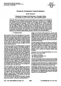
control systems (NCSs), which implement control over communication networks, are becoming increasingly important in industry due to the increasing demand on large-scale integration of information, communications, and control. As shown in Figure 1, an NCS consists of a plant to be controlled, sensors, actuators, and controllers. Sensors, controllers, and actuators are interconnected via a communication network. Introduction to the fundamentals of NCSs can be found in [8–16] and references therein. We have recently analysed the complex behaviour of the network traffic in real-time NCSs, and have found the multifractal nature of the network traffic [3]. The characteristics of non-uniform distribution of the network-induced delay [17] has been used to improve NCS stability analysis by Peng and Tian [18].
Figure 1. Diagram of networked control systems.
It is well realised that control over data networks faces two challenging problems: network-induced delay, and packet dropout. The network-induced delay is time-varying and unpredictable, and thus affects the accuracy of timing-dependent computing and control of the NCSs. The packet loss results from network traffic congestions and limited network reliability, and forces the controller and/or actuator to make a decision on how to control the system when a control packet is lost. Effort has been made to solve these two challenging problems. From Figure 1, it is natural that many control scientists and engineers have focused on the study on the controller side while the network quality-of-service (QoS) conditions are considered as constraints. When the network-induced delay is treated as a stochastic variable, models can be developed to describe the network-induced delay and packet loss, separately or simultaneously. A simultaneous description of both network-induced delay and packet loss in a unified model is considered in [19], and has been shown to be more effective to deal with the network stability and control synthesis [20–25]. With the developed model, stability criteria, which relate to the upper bound of the time delay, are derived that guarantee the stability of the overall NCS [19,22,26,27]. Controller synthesis is also carried out to determine the controller settings under the stability criteria. Packet dropout is considered in some references for establishing the stability conditions, but is not compensated at all. Overall, approaches developed from the perspective of the controller design provide stability conditions, but do not directly deal with the real-time requirement of the NCS network communications. Therefore, conservative control is usually designed in order to guarantee the stability of an NCS. Conventionally, “throwing bandwidth” was an effective method to resolve many problems in network communications. Therefore, some network engineers are optimistic that over-provisioning of network capacity can easily resolve the challenging problems of both network-induced delay and packet dropout. It has not been well recognised in the control community, and also in the networking community, that a high bandwidth does not necessarily mean predictable communication behaviour, and real-time control does not necessarily require fast data transmission. Deterministic communication behaviour is essential in real-time NCS applications. Over-provisioning may work for some applications, but is not a general solution. The reasons are discussed below.
September 10, 2007
5:56
International Journal of Computer Mathematics
TianCompNetV2
LATEX 2ε Dealing with Network Complexity in Real-Time Networked Control
3
(i) There have been many industrial control systems implemented in fieldbus networking, e.g., Controller Area Network (CAN) [7]. However, the fieldbus technology has not been widely accepted in industry so far [28]. Moreover, like all other technologies, fieldbus also has its technical limitations. For example, DeviceNet, a popular fieldbus technique based on CAN provides up to 1Mbps bandwidth with the maximum end-to-end transmission distance of 40m. For 1.3km transmission distance, the bandwidth on the bus is down to 50kbps, implying that only about 25 devices can be interconnected in order to achieve similar performance to that in peer-to-peer networking where each peer-to-peer connection can have up to 1.92kbps bandwidth with RS232 asynchronous communications for about 1km (when using 0-10mA direct current transmission). Over-provisioning of the capacity of such networks is a very expensive solution, if it is not impossible, especially for large scale control systems. (ii) Effort has been made to promote Ethernet based networking for simple and cost effective NCS applications [16, 28, 29]. With recent advances in network technologies, high-speed IP networks have been commercialised with the bandwidth as high as 100Mbps, 1Gbps, and even 10Gbps, so the transmission speed of data in IP networks is no longer a major problem for most industrial applications. However, deterministic and predictable communication performance is not guaranteed in IP networks. If network-induced delay is comparable with the process delay, the performance of the Ethernet based NCS will be largely dependent on the networking. Although high speed Ethernet has very small communication latency [28], it has not been recommended for time-critical NCSs [16] because of its limited real-time QoS. (iii) Our recent studies [10] have shown that for some IP-based NCS networks, simply increasing the network capacity may result in more packet losses for periodic control tasks. We have interpreted this as the consequence of the burst traffic of multiple periodic control tasks. This is not acceptable in many realtime applications, e.g., safety-critical systems. (iv) A large number of sensors and actuators employed in various applications, especially in small and battery-powered embedded control systems, have limited computing power and do not support high communication bandwidth. (v) In wireless networked applications, over-provisioning of the bandwidth is impossible or very expensive in most cases because of the tight bandwidth recourses. Therefore, a general solution to the challenging problems of network-induced delay and packet loss cannot reply on the over-provisioning of the network capacity. From our recent development, this paper aims to develop a general framework to deal with the NCS network complexity. The basic idea is the co-design of network and control. The procedure of the framework is summarised below. • Step 1. Apply a real-time queuing protocol [10, 30] in the NCS network to make the behavior of the network traffic predictable, thus simplifying the network dynamics. The most important achievement is the predictability of the networkinduced delay. • Step 2. Configure the worst-case communication delay (WCCD) under acceptable level of packet loss rate to significantly reduce the network-induced delay in networked control [31]. • Step 3. For any control packet loss, activate a packet dropout compensator, e.g., [4, 32], to predict the lost control signal. A control packet that is received after the control period ends is treated as a lost packet in that control period. • Step 4. Through the above three steps, the network-induced delay is limited within a single control period, largely simplifying the system analysis and design.
September 10, 2007
5:56
International Journal of Computer Mathematics
4
TianCompNetV2
Yu-Chu Tian and David Levy
Then, the predictable network-induced delay is compensated through controller design. Many controller strategies can be used for predictable delay compensation, e.g., [33, 34] The rest of the paper is organised as follows. In Section 2, we rectify our recent development of real-time queuing protocol for networked applications. Section 3 extends our packet dropout compensation scheme. The general framework for dealing with NCS network complexity is summarised and demonstrated through case studies in Section 4. Section 5 concludes the paper.
2. 2.1.
Real-Time Queuing Protocol for Networked Control Queuing Protocol
A few NCS control methodologies have been developed [13]. Among various NCS control methodologies, the ‘queuing methodology’ [35–37] is the only one that aims to develop NCSs with predictable communication timing. The method proposed by Luke and Ray [35, 36] depends crucially on the accuracy of the plant model, ¨ uner [37] is based on probabilistic predictions. and the method by Chan and Ozg¨ However, both have not explicitly addressed the requirement of the predictive timing behaviour of real-time NCS. They have tried to compensate for packet dropout through sophisticated computation at the controller, but these algorithms may not be feasible for implementation at actuators that have limited computing power. Due to these problems, a reference in the open literature to report a successful application of the queuing methods has not been found. Queuing packets to smooth out network-induced delay is not a new idea in multimedia and even in NCS [36,37]. However, the requirement in multimedia applications is different from that in NCS control. For example, throughput is important in video streaming, but is not the focus in networked control as many measurement and control packets are very small. For packet dropout, the existing stability based NCS control methodology does not provide compensation at all; and existing queuing methods have not shown success in real applications. This paper will rectify our real-time queuing protocol to deal with both network-induced delay and packet dropout. Our basic ideas in development of the queuing protocol are: (i) Keep the general networks unchanged at the transport, network, data-link and physical layers to maintain the simplicity, scalability, and interconnectivity of the networks. However, a real-time queuing protocol is introduced on top of the transport layer to meet the real-time communication requirement. (ii) Use two queues to smooth out the network induced-delay and and to compensate for packet dropout. The queuing architecture shown in Fig. 2 implements the above mentioned ideas [10, 30].
Figure 2. Real-time queuing architecture for networked control.
September 10, 2007
5:56
International Journal of Computer Mathematics
TianCompNetV2
LATEX 2ε Dealing with Network Complexity in Real-Time Networked Control
5
Compared with conventional networked control shown in Figure 1, the proposed NCS scheme in Figure 2 has two parallel queues, Q1 and Q2 , at the actuator. Queue Q1 stores only one control packet, and is used to enqueue the received control packet. The enqueued control packet is dequeued from the queue and output to the actuator at a fixed time instant in a control period. In this way, network-induced delay and jitter can be smoothed out. Consequently, the network-induced delay becomes predictable, favorable to real-time networked control. Queue Q2 is a firstin-first-out (FIFO) queue, with a capacity of a few, e.g., two or three, packets. If a control packet is lost, a control signal is estimated from the past control packets stored in Q2 . Using these two queues, we are able to limit the network-induced delay within a single control period, significantly simplifying the NCS analysis and design.
2.2.
Events and Timelines
For periodic control tasks, the events and timelines of the queuing protocol in a control peiod are depicted and explained in Figure 3 [10, 30]. In Figure 3, the earliest possible time instant TE , at which the control packet arrives at queue Q1 , is described by TE = TO + min(tsc ) + tctr + min(tca )
(1)
where min(·) means the lower bound; tsc , tctr , and tca are sensor-to-controller delay, the worst case control computation time, and controller-to-actuator delay, respectively. Without packet dropout, the latest possible time instant TL , at which the control packet reaches queue Q1 , is, TL = TE + tj
(2)
where tj is the sum of sensor-to-controller and controller-to-actuator jitters, i.e., tj = max(tsc ) − min(tsc ) + max(tca ) − min(tca ) where max(·) represents the upper bound.
Figure 3. Timelines for the queuing architecture.
(3)
September 10, 2007
5:56 6
2.3.
International Journal of Computer Mathematics
TianCompNetV2
Yu-Chu Tian and David Levy
Timeline Requirements
The basic requirements among these timeline parameters for real-time systems are:
TO < TE < TL ≤ TC < TD ≤ T.
(4)
Eqn. (4) can be interpreted differently for hard and soft real-time systems, respectively. Hard real-time systems require that Eqn. (4) is always met. Any network design and configurations that do not satisfy Eqn. (4) will not allow the applications of the proposed method in hard real-time systems. However, for soft real-time systems, Eqn. (4) can be occasionally missed out, e.g., TL > T occurs occasionally. This explains why Ethernet has some applications in soft real-time control of industrial processes [28]. It is seen from Figure 3 that TE − TO represents the fixed part of the networkinduced delay and control computing time tctr . It is necessary to optimise control algorithms and network architectures in order to reduce this fixed time delay. The latest time instant for actuators to receive control packets and enqueue them, TL , is chosen such that it covers the major part of the jitter or its full range if possible. In [31], we have shown show how to achieve such a TL under acceptable level of packet loss rate. At time instant TC ≥ TL , check whether queue Q1 is empty or full. For ease of theoretical analysis, we may simply set TC = TL . At time instant TD , dequeue the control packet from Q1 and output the control signal to the plant. The choice of TD relies on how much time is required to deal with control packet dropout. The constraint is that the computing of the algorithm dealing with packet dropout should complete within the time interval TD − TC for hard real-time systems. This constraint can be alleviated occasionally for soft realtime systems.
2.4.
Estimate of Timeline Parameters
In order to check whether the requirements of Eqn. (4) are fulfilled, it is necessary to estimate any two parameters of TE , TL , and tj . Two possible solutions to the parameter estimation are: theoretical calculations and simulation analysis. Eqns. (1) - (3) are expressions of the timing parameters; while more detailed descriptions are required for actual calculations. Theoretical calculations of time delay for simple networks are possible under simplified assumptions [28]. However, such calculations have significant limitations for NCS design. For example, they depends crucially on the configurations of the networks and thus do not scale well. Therefore, we propose to estimate the key timing parameters through network modelling and simulation analysis. With network modelling and simulation, it is easy to analyse the best and worst communication delays under various conditions of network traffic and configurations, such as the timing parameters in Eqns. (1) - (4): TE , TL , max(tsc ), min(tsc ), max(tca ), min(tca ), etc. Moreover, modelling and simulation can also help evaluate the timing behaviours of the NCS network communications. This will be shown in Section 4 through case studies.
September 10, 2007
5:56
International Journal of Computer Mathematics
TianCompNetV2
LATEX 2ε Dealing with Network Complexity in Real-Time Networked Control
3. 3.1.
7
Dealing with Packet Dropout The Concept of Packet Dropout
Packet dropout results from unreliable network interconnections or traffic congestions over the NCS network. Therefore, the problem of packet dropout should be first considered in NCS network design. This is a better option than implementing sophisticated control algorithms to compensate for packet dropout in the control module of the NCS. As a result, sustained sequences of successive dropped packets will unlikely happen under normal conditions in an NCS. From this understanding, substantial packet dropouts might be an indication of abnormal conditions or an unsatisfactory system NCS network design, and should be addressed together with system stability analysis (e.g., [19, 22, 26]) and alarm/safety control modules. This is an issue of the integrated architecture design for the overall NCS, and is beyond the scope of this paper. In the following, we only deal with occasional packet dropouts in an NCS. Basically, there are two types of packet dropouts in an NCS. One is the measurement packet dropout from the sensor to the controller. The other is the control packet dropout from the controller to the actuator. With powerful computing ability, the controller can deal with the measurement packet dropout easily, e.g., through employing complicated predictive algorithms as in [36, 37]. Therefore, we will not discuss how to deal with measurement packet dropout in this paper. We will focus on dealing with control packet dropout. The complicated predictive algorithms in [36, 37] are not directly applicable for control packet dropout. A commonly used methodology to deal with control packet dropout is to derive the maximum allowable network induced delay for NCS stability, e.g., in [19, 22, 26]. However, no any directly compensation has been made for control packet dropout in this methodology - simply do nothing when a control packet dropout happens. In contrary to these existing methods, strategies will be developed in this paper to directly compensate for the control packet dropout. 3.2.
Philosophy for Compensation of Control Packet Dropout
Control packet dropouts refer to the situation where, in a control period, no control packet is received by the actuator before TL , the latest time instant to enqueue a control packet to queue Q1 . Before developing strategies to deal with control packet dropout, we would like to clarify the following two aspects, which are crucial for our development: (i) How much computing power and other resources are available for calculations of packet dropout compensation? (ii) How much chance will various packet dropout scenarios likely occur? To answer the first question we have noted that smart actuators normally have limited computing power and resources, and consequently sophisticated algorithms are difficult to implement in the actuators. Therefore, we have aimed to develop simple and model-free methods to resolve the control packet dropout problem. In this paper, we will further extend our solution presented in [10, 30]. The following discussions help answer the second question. As mentioned previously, an NCS network should be designed such that the packet loss rate is low and sustained sequence of successive dropped packets will unlikely happen under normal conditions. Therefore, it is senseless to discuss how to compensate for, say 50%, packet loss rate, which simply means a bad network design. For a rough quantitative analysis, if the packet loss rate of the network is lr, the rate of s successive
September 10, 2007
5:56 8
International Journal of Computer Mathematics
TianCompNetV2
Yu-Chu Tian and David Levy
packet losses can be estimated as (lr)s . For example, 5% packet loss rate (this is significant for NCS networks), two and three successive packet losses will happen with the chance of 2.5% and 1.25%, respectively. This tells us to focus on the compensation for a single packet loss and two/three successive packet dropouts; there is only a small chance for four or more successive packet dropouts to occur. Compared with the existing methodologies, which either are not directly applicable to control packet dropout compensation (e.g., [36, 37]) or only provide the maximum allowable network induced delay (e.g., [19, 22, 26]), the strategies that will be developed below is innovative in the sense that the control packet dropout is explicitly compensated at the actuators. 3.3.
Strategies to Deal With Control Packet Dropout
The key concepts in our simple solution are: (i) To use the FIFO queue Q2 to buffer a few, e.g., two or three, control packets to allow the smart actuator to recover a dropped control packet; and (ii) To construct a control signal from Q2 when a control packet dropout occurs. Suppose that the control packet in a control period k is not received before time TL , but that there are three control packets, uk−1 , uk−2 and uk−3 , in queue Q2 . We can use these three control packets to construct a packet u ˆk for use in the current control period k. The accent over ‘u’ implies that the packet is an estimate. A simple and general form of u ˆk can be u ˆk = f (uk−1 , uk−2 , uk−3 ),
(5)
where f : R → R is a nonlinear function. A particular choice of f in Eqn. (5) is u ˆk = uk−1 + α∆uk−1 ,
(6)
where ∆uk−1 = uk−1 −uk−2 , and α ∈ [0, 1] is a proportional coefficient. Two special cases of Eqn. (6) are: (1) α = 0; this means u ˆk = uk−1 , i.e., the actuator simply reuses the last control packet queued in Q2 when a control packet fails to arrive; (2) α = 1; it follows that u ˆk = 2uk−1 − uk−2 , i.e., the actuator makes a one-step ahead prediction to the control through a linear extrapolation from the last two control packets queued in Q2 . We have recently analysed the dynamic behaviour of Eqn. (6) through functional analysis using model checking [32]. Duplicating the last control packet, i.e., setting α = 0 in Eqn. (6), provides a conservative control to the plant. Linear extrapolation, i.e., α = 1 in Eqn. (6), gives better control in most cases, but may result in unacceptable behaviour in the presence of repetitive pattern of dropped packets. However, as analysed previously, sustainable and repetitive pattern of dropped packets will unlikely happen under normal conditions (or may happen in very low probability), the simple linear extrapolation is a good choice for compensation for control packet dropout. We have also proposed an adaptive linear extrapolation, which is a further improvement to the linear extrapolation, to predict the control when a control packet is not received by the actuator [32]. The basic idea is to calculate the estimate error which is the difference between the estimate control and the actually received one, and then to use this error to adjust the extrapolated value when a control packet is dropped.
September 10, 2007
5:56
International Journal of Computer Mathematics
TianCompNetV2
LATEX 2ε Dealing with Network Complexity in Real-Time Networked Control
9
More work on packet dropout compensation has also been reported in our recent paper [4], in which past control packets and their derivative information are employed to estimate the lost control packet. As a common industrial practice, preprocessing of measurements and past control packets is necessary in the presence of noises when applying these strategies for packet dropout compensation.
3.4.
Further Analysis of the Strategies
The linear extrapolation strategy shown in Eqn. (6) looks simple. One may argue that this does not seem to be particularly attractive, innovative, or sophisticated either. However, the use of such a simple linear extrapolation can be justified from the following two aspects: (i) The existing methodologies for networked control either do not compensate for control packet dropout at all, e.g., in [19, 22, 26], or attempt to compensate for control packet dropout at the central controller through sophisticated algorithms that may not be feasible for implementation at actuators [36, 37]. The former gives conservative results through robust stability guarantee, while for the latter after 10 years there has been still no reference in the open literature to report a successful application. The simple linear extrapolation proposed in this paper aims to directly compensate for control packet dropout at the actuator that has limited computing power. (ii) The usefulness of a strategy for industrial applications is solely justified by its effectiveness rather than by how sophisticated it is. To build our confidence to use the simple linear extrapolation in Eqn. (6), let us further develop some insight into the strategy. Suppose the measurement series of the controlled variable are yk−1 , yk−2 , yk−3 , · · ·, and a proportional plus integral (PI) controller is used to control the plant. The proportional coefficient and integral time of the PI controller are K and Ti , respectively. It follows that ³ ´ P uk−1 = K ∆yk−1 + T1i k−1 ∆y r r=−∞ ³ ´ 1 Pk−2 uk−2 = K ∆yk−2 + Ti r=−∞ ∆yr ∆yr = yr − yr−1 , r = · · · , k − 2, k − 1
(7)
Substituting Eqn. (7) into Eqn. (6), we have u ˆk = uk−1 +
i αK h ∆yk−1 + Ti (∆t)(∆yk−1 )(1) Ti
(8)
∆yk−1 − ∆yk−2 ∆t
(9)
where (∆yk−1 )(1) =
approximates the derivative of the measurement ∆y at the time instant (k − 1)∆t, ∆t = T is the control period. Eqn. (8) clearly shows that the predicted control action uˆk is a PI+PD (proportional-derivative) predictive control. • The PI part is uk−1 , which is given in Eqn (7); and
September 10, 2007
5:56
International Journal of Computer Mathematics
10
TianCompNetV2
Yu-Chu Tian and David Levy
£ ¤ (1) with the proportional coefficient • The PD part is αK Ti ∆yk−1 + Ti (∆t)(∆yk−1 ) αK Ti and integral time Ti (∆t), respectively. It is a one-step ahead prediction to the control increment. The mode of PI+PD control explains why the linear extrapolation in Eqn. (6) can have good prediction ability. It also reveals the complicated predictive control mechanism behind the simple linear extrapolation.
4.
Case Studies
This section carries out case studies for a middle-scale process or multiple smallscale processes to be controlled over an NCS network, and shows how the real-time protocol proposed in this paper can be applied. The NCS to be modelled and simulated is a TCP/IP network using IEEE802.3 protocols. Switched TCP/IP will be adopted instead of shared-medium TCP/IP, which was investigated by Lian et al [16]. The open source package Network Simulator ns2 [38], which is a discrete event driven simulator for TPC/IP networks, is used to model and simulate the NCS. Because the focus of this paper is on real-time communications for NCSs, we will evaluate the NCS network performance under various scenarios. The issues of controller design and control performance are beyond the scope of this paper and thus will not be discussed here. 4.1.
System Architecture Specifications
The NCS we focus on in the case studies has a three-layer hierarchical topology, as depicted in Fig. 4, which is typical in industrial control systems [39]. The system has been investigated previously in our preliminary studies [10, 30]. On the top of the hierarchy are management computers. Control computers, i.e., controllers, are in the middle. Sensors and actuators, and the plant to be controlled, are at the bottom. There are n smart sensors and m smart actuators, respectively. In practice, n ≥ m. We set n = 30 and m = 20 here to simulate a middle-scale industrial process or multiple small-scale industrial processes. Also, we use 5 control computers and 5 management computers in the NCS.
Figure 4. Hierachical topology of the modelled NCS.
For ease of discussions, we introduce the following notations to represent various devices of the modelled NCS: S1, S2, · · ·, Sn: Smart Sensors, n = 30 A1, A2, · · ·, Am: Smart Actuators, m = 20 C1, C2, · · ·, C5: 5 control computers M1, M2, · · ·, M5: 5 management computers P1, P2, · · ·, Pq: P2P connection devices, q is configurable in our model
September 10, 2007
5:56
International Journal of Computer Mathematics
TianCompNetV2
LATEX 2ε Dealing with Network Complexity in Real-Time Networked Control
11
Table 1. Control Loops.
Loop Sensor(s)
1 1
2 2
... ...
10 10
Actuator
1
2
...
10
11 11 12 11
12 13 14 12
··· ··· ··· ···
20 29 30 20
Without loss of the generality, we assign C1 as the central controller, and C5 as a local control server. C2, C3, and C4 are used for display and other purposes. To evaluate the timing behaviour of the proposed queuing protocol in real-time NCSs, we assume that there are 20 control loops, corresponding to the 20 actuators. The control loops are arranged as in Table 1. Various LAN architecture designs are possible to interconnect NCS hosts and devices. Two such designs are considered in this work: 2Segment and 4Segments configurations both with 10Mbps capacity. In the 2Segment architecture, put all management and control computers in a segment, and all smart sensors and actuators in another segment. In the 4Segment design, we have four segments for management computers, control computers, sensors, and actuators, respectively. These two architecture designs with their representations in ns2 are shown in Figs. 5 and 6, respectively.
Figure 5. 2Segment architecture (upper) and its simplified ns diagram (lower) for the modelled NCS.
Figure 6. 4Segment architecture (upper) and its simplified ns diagram (lower) for the modelled NCS.
September 10, 2007
5:56
International Journal of Computer Mathematics
12
4.2.
TianCompNetV2
Yu-Chu Tian and David Levy
Traffic Flow Specifications
For traffic flow specifications, we suppose that control tasks are periodic with the period of 200ms. Typical traffic flows in the NCS are specified below. (i) Within a control period, each of the smart sensors sends a packet of 200 bytes in the first 50ms to the controller (C1), and also to the local server (C5). (ii) From 100ms to 200ms, the controller sends a control packet of 200 bytes to each of the actuators, and a packet of 1k bytes to the local server C5. (iii) In each control period, C5 sends packets of 2k bytes to each of C2, C3, and C4 for local information processing, monitoring, and displaying. (iv) Each of C2, C3, and C4 sends queries to the local server C5 and gets responses from C5 within an interval of 5s. The sizes of the queries and responses for each of C2, C3, and C4 are 1k and 10k bytes, respectively. (v) Within a session of 10min, each management computer sends queries of 60k bytes to the local server C5, and gets responses of 600k bytes from C5. From the above specifications, traffic flows are calculated and tabulated in Table 2 for the modelled NCS. It is worth mentioning that for each TCP packet transmitted over the NCS network, there is a 40-byte overhead for TCP and IP headers. Table 2. Traffic Flow Specifications.
No. Traffic Flow Flow Rate TCP1. 0–50ms: each S1 ∼ Sn ⇒ C1 200 bytes → 8kbps TCP2. 0–50ms: each S1 ∼ Sn ⇒ C5 200 bytes → 8kbps TCP3. 100–200ms: C1 ⇒ each A1∼Am 200 bytes → 8kbps TCP4. 100–200ms: C1 ⇒ C5 1k bytes → 40kbps TCP5. 0–200ms: C5 ⇒ each C2∼C4 2k bytes → 80kbps TCP6. 0–5s: each C2∼C4 ⇒ C5 1k bytes → 1.6kbps TCP7. 0–5s: C5 ⇒ each C2∼C4 10k bytes → 16kbps TCP8. 0–10min: each M1∼M5 ⇒ C5 60k bytes → 800bps TCP9. 0–10min: C5 ⇒ each M1∼M5 600k bytes → 8kbps Packet Size (bytes) - TCP1,2,3,6: 200; TCP4,5,7,9: 1k; TCP8: 100 10Mbps capacity and 4ms propagation time for all links
In all cases, assume that the network propagation time is 4ms for all LANs and P2P links. For each of the case studies, the modelled NCS is simulated for 10s using ns2 under Unix. All traffic flows over the network are monitored and recorded in trace files. Then, extract information from the trace files and analyse and evaluate the performance the NCS network. 4.3.
Case Study 1: TwoSegments/10Mbps
This case study, as shown in Fig. 5 for 10Mbps capacity, has been investigated in our preliminary work under different configurations [10, 30]. Selected results of our simulation and performance analysis are summarised in Table 3. The first observation from Table 3 is that all measurement and control packets are successfully delivered to their destinations. This implies that the NCS network is reliable for NCS communications under the modelled conditions. The second observation from Table 3 is that the sensor-to-actuator delay ranges from 16.30ms to 93.34ms, and the controller-to-actuator delay changes from 16.93ms to 34.16ms. Considering both sensor-to-controller delay and controller-toactuator delay, we can see that the total NCS communication latency is between
September 10, 2007
5:56
International Journal of Computer Mathematics
TianCompNetV2
LATEX 2ε Dealing with Network Complexity in Real-Time Networked Control
13
Table 3. Case study 1 (2Segments/10Mbps): performance analysis.
Total number of recorded receive events: 25 600 All measurement/control packets received? Yes Received bits/s within each local area (bps) Network Utilisation Computer side: 1 313 760 < 13.2% Sensor/actuator side: 901 120 < 9.1% P2P link: 901 120 < 9.1% Average throughput (bps): C1 C5 Aj (Actuator) 323 232 355 680 9 632 Sensor-to-controller delay and jitter (ms) S01 S10 S20 S25 S30 All Min delay 16.64 16.71 16.71 16.71 16.81 16.30 Max delay 69.79 77.92 93.34 91.04 56.65 93.34 Jitter 53.15 61.25 76.64 74.33 39.84 77.05 Controller-to-actuator delay and jitter (ms) A01 A05 A10 A15 A20 All Min delay 17.50 17.35 18.42 19.48 19.12 16.93 Max delay 28.92 29.85 31.37 32.86 34.16 34.16 Jitter 11.42 12.50 12.96 13.38 15.04 17.23 33.23ms and 127.50ms, resulting in a jitter of 94.27ms. Both the latency and jitter are significant. Using the notations in Eqns. (1) through (4), we have min(tsc ) = 16.30ms, max(tsc ) = 93.34ms min(tca ) = 16.93ms, max(tca ) = 34.16ms tj = 94.27ms
(10)
These rough estimates will be used later for calibration of timeline parameters in our queuing protocol for real-time NCSs. To show how significant the communication latency and jitter are in the NCS, Figs. 7 and 8 depict the plots of sensor-to-controller delay and its distribution, respectively. Fig. 7 shows that the sensor-to-controller delay exhibits irregular dynamic behaviour. Such behaviour has been traditionally treated as randomness in NCS research. However, our recent work has revealed the multifractal nature of the network induced time delay in such NCSs, implying that the time delay is long-range correlated [3].
Figure 7. Sensor-to-controller delay for case study 1.
Compared with the sensor-to-controller delay, the control-to-actuator delay, as shown in Fig. 9, exhibits more regular behaviour with small jitter. This is due to the
September 10, 2007
5:56 14
International Journal of Computer Mathematics
TianCompNetV2
Yu-Chu Tian and David Levy
Figure 8. Distibution of the sensor-to-controller delay for case study 1.
same setting of the control period for all control tasks in the NCS; and the setting means that there is no sensor-to-controller traffic sharing the network bandwidth when the controller is sending control packets to the actuators.
Figure 9. Delay from the controller to actuator 10 for case study 1.
Now let us show how to use the rough estimates in Eqn. (10) to calibrate the timeline parameters in our queuing protocol. We have set the control period T = 200ms. For timeline settings in Fig. 3 and Eqns. (1) through (4), let TO = 0ms. From Eqns. (1) and (10), it follows that TE = 33.23ms + tctr = 88.23ms
(11)
where tctr = 50ms is the control computing time. We will try to cover the full range of the communication jitter to avoid any control packet dropouts. According to Eqns. (2), (3), (10) and (11), we need to set TL ≥ TE + tj = 127.50ms + tctr = 177.50ms.
(12)
For the control period of 200ms, it is seen from Eqns. (4) and (12) that we still have around 22.50ms for checking the queue Q1 , dealing with possible packet dropout, and outputting the control action to the plant. In this example, we can simply set TC = 180ms, TD = 190ms.
(13)
This will allow extra TC −TL = 2.50ms time for control computing (tctr ) and packet transmissions. We also have TD − TC = 10ms time to deal with possible packet dropout. The total time delay for the control computation and packet transmission
September 10, 2007
5:56
International Journal of Computer Mathematics
TianCompNetV2
LATEX 2ε Dealing with Network Complexity in Real-Time Networked Control
15
in each of the control loops is TD = 190ms, which is fixed for all control periods. Fig. 10 shows the resulting timing behaviour of the modelled NCS (Refer to Table 1 for control loop arrangement). It is seen from Fig. 10 that deterministic and predictable timing behaviour is achieved for the NCS by using the proposed queuing protocol.
Figure 10. Timing behaviour of the NCS with the queuing protocol for case study 1 (‘O’: measurement packets received by controller; ‘X’: Control packets received by the actuator; ‘*’: TC ; ‘∆’: TD ).
4.4.
Case Study 2: FourSegments/10Mbps
Simulation results for the case study FourSegments/10Mbps as shown in Fig. 6 are summarised in Table 4 [10]. Table 4. Case study 2 (4Segments/10Mbps): performance analysis.
Total number of recorded receive events 34 420 All measurement/control packets received? Yes Received bits/s within each local area (bps) Network Utilisation Control computer side: 1 313 760 13.1% Manag. comput. side, P2-P5: 51 040