Decentralized Cascade Control of Binary Distillation

ThP10.1

Proceeding of the 2004 American Control Conference Boston, Massachusetts June 30 - July 2, 2004

Decentralized Cascade Control of Binary Distillation Columns Eduardo Castellanos-Sahagún and Jesús Alvarez* Universidad Autónoma Metropolitana, Unidad Iztapalapa Departamento de Ingeniería de Procesos e Hidráulica Apdo. Postal 55534, 09340, México D. F., MEXICO ABSTRACT In this work the problem of designing a two-point (temperature-composition) linear decentralized cascade controller for binary distillation columns is addressed within a nonlinear robust constructive control framework, yielding: a systematic construction, a simple tuning scheme coupled with a robust stability criterion, an inputoutput pairing criterion based on RGA-like (relative gain array) analysis, and the identification of the performance limiting factors. The proposed approach is illustrated with a benchmark representative example and numerical simulations, showing that the proposed linear decentralized cascade design can recover the performance of its MIMO counterpart (Castellanos-Sahagún and Alvarez, 2004), which in turns recovers the performance of an exact model-based nonlinear state-feedback composition controller. 1. INTRODUCTION Distillation represents the most used separation operation and since it is energy intensive, the development of improved control techniques for these processes constitutes a relevant problem. Designing dual composition controllers is challenging, because of strong nonlinear interaction, and ill-conditioning, mostly in high purity columns. Usually, the control approach taken is to design decentralized (i. e., diagonal) controllers (Niederlinski, 1971; Skogetsad, 1997 and references therein), which are tuned as two linear independent SISO loops. The diagonal input-output parings are chosen according to relative gain array (RGA) techniques, the interaction conflict is usually handled via integral action plus loop detuning (Ogunnaike et. al., 1994), sacrificing performance. The structure-oriented nonlinear geometric control theory (Isidori, 1995) offers rigorous means to address the interaction problem. In fact, dual composition control has been investigated in this framework. If the composition measurements are on-line available, the construction of a nonlinear geometric dual composition control can be carried out easily, because the associated relative degrees _______________________________________________ * Corresponding Author: [email protected]

0-7803-8335-4/04/$17.00 ©2004 AACC

are equal to one. This has been done using low order models (Castro et. al., 1990, Lévine et. al. 1991), and nonlinear wave models (Balasubramhanya et. al., 1997), in conjunction with suitable state estimators. However, these composition controllers have two drawbacks, especially in high-purity separations: (i) the low sensitivity of the composition outputs with respect to input disturbances and controls, and (ii) the control actions take place after the disturbances have upset the entire composition profile. To cope with these problems, two-point decentralized (Wolff and Skogestad, 1996; Alvarez-Ramírez et al. 2002) and MIMO (Shin et. al., 2000; Castellanos-Sahagún and Alvarez, 2003 & 2004) cascade control schemes have been proposed. A fast secondary temperature loop compensates quickly the effect of disturbances on the composition profile, while a slow primary composition controller yields the temperature setpoints, regulating effluent compositions. However, it is not clear whether the extension to the cascade case of the optimal linear decentralized composition controller (Morari et. al., 1989) can adequately handle the loop interaction conflict. Wolff and Skogestad (1996) studied this problem, and concluded that the use of two composition-temperature cascaded loops is not advisable, at least for a specific column. Nevertheless, three recent studies have successfully addressed this two point cascade control problem: (i) Shin et. al. (2000) combined a linear decentralized primary controller with a nonlinear (reduced-order wave model) observer-based secondary controller, (ii) Alvarez-Ramírez et. al. (2002) combined a linear decentralized cascade design with a linear observer-based modeling error compensator in the secondary loop, and (iii) Castellanos-Sahagún and Alvarez (2004) proposed a linear MIMO cascade controller, with observer-based modeling error compensation in both the primary and the secondary loops. In the latter work, a linear MIMO cascade recovered the performance of a nonlinear state feedback (SF) composition-only controller, with the gain limiting factor the presence of high-frequency dynamics, mainly holdup dynamics (also known as hydraulics, or liquid flow dynamics, Skogestad, 1997). Knowing that a linear MIMO cascade controller can recover the behavior of a nonlinear SF composition controller (Castellanos-Sahagún and Alvarez 2004), and keeping in mind the industrial success and acceptance of decentralized controllers, in this work is investigated if the 3556

same behavior recovery can be accomplished with a decentralized cascade controller. In the present work, we show that this question is positively answered, the linear decentralized cascade control of distillation columns is addressed within a nonlinear robust constructive control framework (Krstić et al., 1995; Sepulchre et al., 1997) based on the notions of passivity and observability of unknown inputs due to unmodeled dynamics. The I/O pairings are carried out in the light of relative gain array-like (RGA, Bristol, 1966) tools, and the decoupling matrix associated to the output controllability property. The solvability conditions and the closed-loop robust stability issues are discussed, and simple tuning guidelines are provided. The proposed approach is tested with numerical simulations, showing that the proposed linear decentralized cascade controller can recover the performance of its MIMO counterpart (Castellanos-Sahagún and Alvarez, 2004), which in turns recover the performance of a nonlinear SF one, the main gain limitation due to the presence of holdup dynamics. 2. CONTROL PROBLEM Consider a binary distillation column with N trays plus reboiler and condenser, where a binary mixture is fed at tray nf, with molar flow F and composition cF, yielding flows B (bottoms) and D (distillate), with compositions co and cD respectively. The objective is to maintain (co, cD), by regulating the temperatures in two trays (to be chosen), using the well known RV configuration (Skogestad, 1997). The measured outputs are the temperatures Ts and Te, in the stripping (and enriching) section of the column, respectively, as well as the composition of the bottom effluent, and of tray N. The reason for measuring cN instead of cD is explained in Castro et. al. (1990): when cD is measured, the decoupling matrix (Isidori, 1995) is singular. From standard assumptions (constant pressure; equilibrium in all trays; perfect level control, constant molar flows), the column dynamics are given by: -1 . c0 = {η(m1)(c1 - c0) + V[c0 - ω(c0)]}m0 . ci = {η(mi+1)(ci+1 - ci) + V[ω(ci-1) - ω(ci)] -1 1≤i≤N-1 + δi,n F(cf - ci)}mi , f

-1 . cN = {R(cD - cN) + V[ω(cN-1) - ω(cN)]}mN -1 . cD = V[ω(cN) - cD]mD . mi = η(mi+1) - η(mi), 1 ≤ i ≤ N, η(mN+1) = R T

T

c

c

ψs = σ(cs), ψe = σ(ce), ψo = λo(co), ψN = λN(cN) λo(co) = ln(co), λN(cN) = -ln(1 - cN) where δi,n is Kronecker’s delta, ci (or mi) is the light f component mole fraction (holdup) at the i-th stage, ω σ and η are respectively the nonlinear liquid-vapor equilibrium, T T bubble point and the hydraulic functions; ψs (or ψe ) is the temperature measurement in the s-th (or e-th) tray in the

stripping (or enriching section). To improve primary control behavior, yco (or ycN) is chosen as the logarithmic composition measurement (Shinskey, 1988) in the 0-th and N-th trays. For control design purposes, we assume constant holdups, in the understanding that the application example will include holdup dynamics (Skogestad, 1997; Castellanos-Sahagun and Alvarez, 2004). In compact notation, the n-state (n=N+2), 2input, 4-output, reduced column model is given by: . c = F(c, δ, υ), ψT = hT(c), ψc = hc(c) (1) c = (c0, c1 ,…, cN, cD)', δ = (F, cF)', υ = (V, R )' hc(c) = [λo(co), λN(cN)]' hT(c) = [σ(cs), σ(ce)]', At the nominal steady state operation (c-, δ, υ- ), the following algebraic equations are satisfied: 0 = F(c-, δ, υ- ),

ψ- T = hT(c-),

ψ- c = hc(c-)

(2)

Our cascade control problem consists in designing a decentralized linear dynamic cascade controller to regulate the output concentrations (ψc) by means of a slow primary controller that yields the temperature setpoint vector (ψ*T) of a fast secondary controller that steers the control input vector (υ). In particular, we are interested in: (i) drawing a systematic design methodology with a simple tuning scheme, coupled to a closed-loop robust stability criterion, (ii) identifying the I/O pairs for decentralized control, (iii) and putting our approach in perspective with the existing linear and nonlinear cascade control designs. 3. CONSTRUCTIVE CONTROL FRAMEWORK 3.1 Coordinate Change The application of the relative degree algorithm (Isidori, 1995) to the reduced column model (2), leads to the following conclusions: (i) the secondary input-output pair (yT, u) has a (passive) relative degree (1, 1), and (ii) the primary input-output pair (yc, yT) has a (non-passive) relative degree (s, N - e). This means that the secondary SF (state feedback) controller problem admits a robust solution, and that the same is not true for the primary controller because its construction involves high (s, and N-e) order derivatives of the nonlinear uncertain functions ω and σ. Following the constructive control paradigm, Sepulchre, Janković and Kokotović, 1997), the high degree obstacle is removed via the derivation of a linear passive realization of the model. First, let us introduce the next (deviation) coordinate change x(c) = (x' , x' , x')', x = [λ (c ) - λ (c- ); λ (c ) - λ (c- )]' c

T

I

c

o

o

xT = [σ(cs) - σ(c-s); σ(ce) - σ(c-e)]',

o

o

N

N

N

xI = (cI - c-I)' cI = [c1,..., cs-1, cs+1,..., ce, ce+1, cN-1, cN+1]' - , y =ψ -ψ d = δ - δ, u = υ - υ- , y = ψ - ψ T

T

T

c

c

N

c

to take the column into (linear in the output) nonlinear system . xc= fc(xc, xI, d, u), yc = xc . xT = fT(xT, xI, d, u), yT = xT 3557

. xI = fI(xc, xT, xI, d, u),

dim(xI) = n-4

(3)

3.2 Decoupling Matrices Now, take the directional derivatives of the output maps (matrices and nonlinear maps are defined in the Appendix): . . yc = fc(x, d, u); yT = fT(x, d, u) (4) The decoupling matrices (Isidori, 1995) associated with the pairs (u, yc), and (u, yT) are given respectively by (Castellanos-Sahagún and Alvarez, 2003): Ac = ∂ufc(0, 0, 0) = DcP; AT = ∂ufT(0, 0, 0) = DTP D = diag{(c- - c- )/(c- m ), (c- - c- )/[(1 - c- )m ]} c

1

o

o

o

D

N

N

N

DT = diag{σ′(c-s)(c-s+1 - c-s)/ms, σ′(c-e)(c-e+1 - c-e)/me} - ps 1 - - - pe = R/V P = ⎡⎣- p 1⎤⎦, ps = (R+F)/V, e

(5) where ps ≥ 1, pe ≤ 1, are the slopes of the stripping and enriching section operating lines in the corresponding nominal McCabe-Thiele design diagram. As shown in our previous work, (Castellanos-Sahagún and Alvarez, 2004), P is nonsingular if ps ≠ 1, and pe ≠ 1 (ps = pe = 1 at infinite energy, or equivalently, minimum number of stages, Skogestad 1997). Necessarily, the nonsingularity of DT requires a temperature measurement in each section of the column, preferably allocated where the maximum tray-to-tray temperature change occurs (Castellanos-Sahagún and Alvarez, 2003). The diagonal elements of the diagonal matrix Dc can be close to zero, especially in high-purity columns with a large number of trays, and this could limit the performance (i.e., small gains should be used to avoid error propagation). The nonsingularity of the decoupling matrix Ac (or AT) is equivalent to the output controllability property (Chen, 1984) of the column with the output yc (yT). Thus, these matrices contain the input-output (I/O) interaction information that is relevant for a linear cascade control design with passive relative degrees. 3.3 I/O Pairings Usually, a RGA (relative gain array, Bristol, 1966) analysis can be applied to an input-to-output transfer function of a MIMO process. Here we apply a similar analysis to the static decoupling matrices (which can be seen as the input-to-output time derivative static transfer function). The resulting interaction parameters ρ are equal for both decoupling matrices: - ρ(Ac) = ρ(AT) = 1/(1 - pe/ps) = 1 + R/F > 1 (6) This expression with ρ > 1, says that the best pairings are those in the diagonal, since pairings with negative RGA parameters should be avoided (Skogestad, 1997; Shinskey, 1988). This is consistent with previous findings (Sågfors and Waller, 1998). Thus, according to the RGA parameter, in the light on the interaction feature associated to the output

controllability property, the best pairings for decentralized control are: (y0, V) and (yN, R) for the composition loop, and (ys,V) (ye, R) for the temperature loop. Such pairings agrees with previous ones (Skogestad and Morari, 1988; Skogestad and Lundström, 1990; Wolff and Skogestad, 1996), drawn from the application of the RGA to the I/O transfer function of the column. 3.4 Linear Decentralized Realization In terms of the (nonsingular) diagonal approximations Ac and AT of the (squared) decoupling matrices Ac and AT: A = diag{-p (c- - c- )/(c- m ), (c- - c- )/[(1 - c- )m ]} c

s

1

o

o

o

D

N

N

N

AT = diag{-psσ′(c-s)(c-s+1 - c-s)/ms, σ′(c-e)(c-e+1 - c-e)/me}

(7)

the distillation column dynamics can be rewritten in the next linear-nonlinear interconnected systems form (see figure 1): . xc = Acu + bc, yc = xc (8) . xT = ATu + bT, yT = xT . xI = fI(x, d, u), bc = βc(x, d, u), bT = βT(x, d, u) βc(x, d, u) = fc(x, d, u) - Acu, βT(x, d, u) = fT(x, d, u) A Tu (βc, βT, fI)'(0, 0, 0, 0, 0) = (0, 0, 0)' This system is made by the interconnection of two linear decentralized controllable subsystems, and a nonlinear unmodeled one. Each linear subsystem is controllable, and the state-input pairs (xc,bc), (xT,bT) are instantaneously observable (Hermann et. al., 1977), because they can be reconstructed from the measurement yc (or yT) and its . . derivative xc (or xT). Therefore, the effect (bc or bT) of the "unknown" dynamics xI on the linear subsystem xc (or xT) can be reconstructed arbitrarily fast, via a dynamic observer, and as a consequence, we can assume they are known for observer-based control design purposes.

C o n tro l M o d e l yc = xc

.

x c = A cu + bc u

yT = xT

.

x T = A Tu + bT

b T, b c

xc, x T

u

.

xι

x ι = f ι (x , d , u ) d

β c( x , d , u ) β T (x , d , u ) d

u

U n m o d e le d d yn a m ics

Figure 1. Distillation Column in linear-nonlinear interconnected form

3558

3.5 Linear Decentralized Control Model Knowing that any robust linear controller can be realized in observer-controller form (Zhou, 1998), let us consider the following internal linear decentralized model: . . xc = Acu + bc, bc ≈ 0, yc = xc (9) . . bT ≈ 0, yT = x T (10) xT = ATu + bT, where the unknown but observable input bc (bT) is regarded as an augmented dynamical state with a rate of change that is slow when compared with the observer (to be constructed) dynamics. This model is consistent with the Internal Model Principle (Wonham, 1985) which states that “to compensate the effect of the unknown disturbances (bc, bT) generated by an unknown exosystem (i.e., the unmodeled dynamics), the controller must include an exosystem model”. 4. LINEAR DECENTRALIZED CASCADE CONTROL 4.1 Cascade SF-Controller To build the cascade controller, we must find a temperature setpoint vector that ensures that the measured compositions track the desired setpoints. For this aim, impose the closedloop decoupled composition regulation dynamics (ωc is the primary loop gain): . xc = - Kcxc,

Kc = diag(ωc, ωc)

(11)

in (9a) and solve for u to obtain the "virtual" controller: -1

uc = Ac (- Kcxc - bc),

(12)

The application of this controller to the temperature equation of the internal model (10) yields the decentralized primary controller (i.e., the setpoint generator): -1 . xT* = ATAc (- Kcxc - bc) + bT

(13)

-1

where ATAc is a diagonal matrix. To build the secondary controller, let us enforce the first order decoupled temperature dynamics in (10): . . xT - x*T = - KT(xT - x*T),

- i) The matrices Ac, AT have inverses, or equivalently, |P| ≠ 0, |Dc| ≠ 0, |DT| ≠ 0 (see section 3). ii) The stability of origin of the (n - 2)-dimensional (internal) zero-dynamics (i.e, (12) with xc = 0, under the -1

control uc = -Ac bc) . xI = ΦI(0, x*T, xI, d), . xT* = ΦT(0, x*T, xI, d)

(14)

(ωT is the secondary controller gain), and solve for u: -1 . u = AT [x*T - KT(xT - x*T) - bT], (15) 4.2 Solvability Conditions As stated in Castellanos-Sahagún and Alvarez (2003), using well known nonlinear geometric control arguments (Isidori, 1995), the necessary and sufficient conditions for the solvability of the cascade SF-controller are:

(16)

iii) The secondary controller is tuned sufficiently faster than the primary one (ωT ≥ ωc). Condition (i) is met if: (a) the slopes of the operating lines are different (ps ≠ pe). (b) Diagonal elements of Dc can be very small numbers (c) DT will be nonsingular if its diagonal elements σ´(c-s)(c-s+1 - c-s) ≈ Ts+1 - Ts ≠ 0 σ´(c- )(c- - c- ) ≈ T - T ≠ 0 e

e+1

e

e+1

(17)

e

As (17) shows, the numerators of the elements of DT are approximately the temperature gradients in the chosen trays. To obtain a well-conditioned matrix, the measurements trays should be those where the maximum tray to tray change occurs in each section of the column. Physically speaking, the condition (ii) means that the plant -1

is stable under the material balance control uc = -Ac bc. Condition (iii) is required to enhance the control response, i.e., the secondary controller is intended to reject load disturbances before the latter ones affect the output compositions. 4.3 Measurement-Driven Cascade Controller The combination of the open-loop observers (eq. 18), associated to the linear internal model (eqs. 9, 10), with the cascade controller (eqs. 13, 15) yields the measurementdriven controller in IMC form (ζ is a damping factor of the second order observer, and ωo is the observer gain): Internal model:

(18)

.

.

P

x^c = Acu^ + ^ bc +

KO (yc - x^c),

.

P

b^c = KI (yc - x^c)

.

x^T = ATu^ + ^ b T + KsO (yT - x^T), b^T = KsI (yT - x^T) P P Ks = K = 2ζω diag(1,1), Ks = K = ω 2diag(1,1) O

KT = diag(ωT, ωT)

xI(t = 0) = xIo

o

O

I

Control

.

I

-1

x^T* = ATAc [ - Kcx^c - ^ b c] + ^ bT -1

-1

u^ = Ac ( - Kcx^c - ^ b c) -AT KT(x^T - x^*T )

o

(19) (primary) (secondary)

4.4 Closed-Loop Stability and Tuning The closed-loop error dynamics of the nonlinear column (2) with the dynamic output feedback cascade controller (18-19), is given by the following equations:

3559

(20) ΩI(0, 0) = 0 Ωc(0) = 0

ΩT(0) = 0 Ω*T(0) = 0 θe(0, 0, 0, 0, 0) = 0

where ε*T = x^T - x^*T, and xc, are the regulation errors, and ε is the observation error. Moreover, with (θe, Ω*T, ΩT, Ωc, ΩI) = 0, the individual subsystems (x, ε*T, ε) are stable. From singular perturbation arguments (Kokotović et. al., 1986), and the vanishing properties of (θe,Ω*T, ΩT, Ωc, ΩI), follows that the preceding closed-loop system is stable if the observer is tuned sufficiently faster than the secondary controller, which in turn must be tuned faster than the primary one. This is ωo > ωT > ωc such that the estimation, secondary and primary controller dynamics are sufficiently separated. The presence of (parasitic high frequency) holdup dynamics limits the observer and controller gains, as shown in CastellanosSahagún and Alvarez (2004). In that work it was proven that with any nonsingular approximations of Ac and AT, the linear decentralized controller recovers the behavior of an exact model-based nonlinear SF composition controller. The preceding results lead us to the following tuning guidelines. Keeping in mind the level of measurement noise and the unmodeled high-frequency dynamics (mainly holdup dynamics):

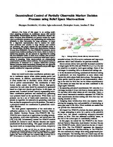
ωp = 0.0.4 min-1. We compare the performance of the proposed approach with the one of the previous MIMO linear cascade control of Castellanos-Sahagún and Alvarez (2004) (with ωo = 0.89 min-1, ωs = 0.267 min-1, ωp = 0.133 min-1). Figure 2 shows the closed-loop (CL) response of both controllers to a sequence of step disturbances. At t = 0 minutes, the column is subjected to a step perturbation in feed composition, from 0.5 to 0.2. Then at t = 200 minutes, there is -30% step change in feed flow rate. At t = 400 minutes, feed composition steps from 0.2 to 0.5. Finally, at = 600 min, feed rate returns to its nominal value. From the figure we can see that the proposed linear decentralized cascade controller yields a behavior similar to the aforementioned MIMO controller, with recovery times of about 50-60 min (i.e, 0.250.3 natural settling times, if we consider that this column has a response time of about 200 min). As stated before, the presence of (high-frequency) holdup dynamics limits the observer and controller gains (e.g., if higher observer and controller gains are used, the response becomes oscillatory; nevertheless, the output compositions are still regulated properly). On the other hand, if slower observer and controller gains are used, the response degrades (i.e., the deviations, and the recovery rates are larger). This was shown in the previous study of Skogestad and Lundström (1990), where the use of more conservative gains and integral times in their decentralized PI composition controllers degraded the performance. Comparing with the existing linear and nonlinear controllers (Skogestad and Morari, 1988; Shin et. al., 2000), the proposed controller yields a faster recovery with smaller deviations, meaning that the successful optimal composition control design (Morari et. al., 1989) can be effectively extended to the cascade case. 0.02 Bottoms composition cB

Closed-loop reduced model . xI = ΦI(xc, x*T, xI, d) + ΩI (ε, ε*T), -1 . xc = - Kcxc- AcAT KTεT* + Ωc(ε), . xT* = ΦT(xc, x*T, xI, d) . . xT = x*T + KTε*T + ΩT(ε) . ε*T = - KTε*T + Ω*T(ε), . ε = Aoε + πθε(ε, xc, xT, xI, d),

0.01

-1

behavior is attained, in the understanding that ωc|Ac | ≈ 1 limits the gain ωc. 5. APPLICATION EXAMPLE As a representative example, let us consider Morari et. al.’s (1989) distillation column A, including the holdup dynamics described in Wolff and Skogestad (1996). The application of the sensor allocation criterion (17) yields that the temperature measurement trays are s = 13 (stripping section), e = 24 (enriching section). The application of the tuning guidelines yielded in a rather straightforward manner ζ = 3, ωo = 4 min-1, ωs = 0.67 min-1,

0.00

Distillate composition cD

(i) Tune the observer gain ωo as fast as possible (ii) With the primary controller disconnected (ωc = 0), tune the secondary temperature controller as fast as possible, typically at least 3 - 10 times slower than the observer (ωT ≈ 1/10 - 1/3ωo). (iii) Increase the primary control gain ωc until a satisfactory

1.00

0

200

400

600

800

MIMO control Decentralized control 0.99

0.98 0

200

400

600

800

Time, minutes

Figure 2. Response comparison between the proposed cascade decentralized controller and a linear MIMO one, to a sequence of step disturbances.

3560

A methodology for the constructive design of two-point decentralized cascade controllers for binary distillation columns has been developed, including a systematic construction, a tuning scheme coupled with a stability criterion, the election of the best pairings for decentralized control, and the property of recovering the behavior of an exact model based nonlinear SF composition controller. The methodology is consistent with widely used heuristic knowledge, and identifies a connection between linear and nonlinear control techniques.

Skogestad, S., Lundström, M. Computers & Chem. Engng., Vol. 14, No. 4/5, pp. 401-413 (1990). Skogestad, S., Morari, M. CES Vol. 43, No. 1, pp. 33-48 (1988). Tolliver, T. L., McCune, L. C. InTech, Vol. 27. No. 9, pp. 75-80. (Sept. 1980). Wolff, E. A., Skogestad S.. I & EC Res., Vol. 35, pp. 475484 (1996). Wonham, W. M. Linear Multivariable Control: A Geometric Approach. 3rd Ed. Springer (1985). Zhou, K. Essentials of Robust Control. Prentice Hall (1998).

BIBLIOGRAPHY

APPENDIX

6. CONCLUSIONS

Alvarez-Ramírez, J., Monroy-Loperena, R., Alvarez, J. AIChE, J., Vol. 48, No. 8, pp. 1705-1718 (2002). Balasubramhanya, L. A., Doyle III, F. J. AIChE J., Vol. 43, No. 3, pp. 703-714 (1997). Bristol, E. IEEE TAC, Vol. 11, pp. 133-134 (1966). Castellanos-Sahagún, E., Alvarez, J. Proc. of the 2003 ACC, Denver Co., pp. 373 - 378 (2003). Castellanos-Sahagún, E., Alvarez, J. “An Adaptive Cascade Multivariable Controller for a Class of Binary Distillation Columns” Submitted to International Journal of Adaptive Control and Signal Processing (2004). Castro, R., Alvarez, J, Alvarez, J. Automatica, Vol. 26, No. 3, pp. 567-572 (1990). Chen, C. T. Linear System Theory and Design. Harcourt Brace College P., New York, 1984. Hermannm, R., Krener, A. J.. IEEE TAC, AC-22, No. 5, pp. 728-740, (1977). Isidori, A. Nonlinear Control Systems. An Introduction, 2nd Ed. Springer-Verlag, (1995). Kokotović, P. , Khalil, H. K., O’Reilly. Singular Perturbation Methods in Control: Analysis and Design. Academic Press (1986). Krstić, M., Kanellakopoulos, I., Kokotović, P. Nonlinear & Adaptive Control Design. Wiley, (1995). Lévine, J., Rouchon, P. Automatica, Vol.27, pp. 463-480 (1991). Morari, M, Zafiriou, E. Robust Control. Prentice-Hall (1989). Niederlinski, A.. AIChE J., Vol. 17, No. 5, pp. 1261-1263 (1971). Ogunnaike, B. Ray, H. Process Dynamics, Modeling & Control. Oxford Univ. Press (1994). Sepulchre, R., Janković, M., Kokotović, P. R. Constructive Nonlinear Control. Springer Verlag, London (1997). Sågfors, M. F., & Waller, K. V. J. Proc. Cont. Vol. 8, No. 3, pp 197-208 (1998). Shin, J. Seo, H., Han, M., & Park, S. CES Vol. 55, pp. 807813 (2000). Shinskey, G. Process Control Systems, 3rd Ed. McGrawHill (1988). Skogestad, S. Modeling, Identification & Control Vol. 18, No. 3, pp. 177-217 (1997).

. . θc(xc, xT, xI, ε*T, ε, d) = (∂βc/∂xc)xc + (∂βc/∂xT)xT

. . . + (∂βc/∂xI)xI + (∂βc/∂u)u^ + (∂βc/∂d)d . . θT(xc, xT, xI, εT* , ε, d) = (∂βT/∂xc)xc + (∂βT/∂xT)xT . . . + (∂βT/∂xI)xI + (∂βT/∂u)u^ + (∂βT/∂d)d .

-1

P

P

u^ = Ωu(x, ε*T, ε) = Ac {- Kc[- Kc(xc + εc) + KOεc] - KI εc} -1

- AT KT[-KTεT* + ΩT* (ε)] Observation errors ε = (εc1, εbc1, εc2, εbc2, εT1, εbT1, εT2, εbT2)' εc1 = x^c1 - xc1, εc2 = x^c2 - xc2, εT1 = x^T1 - xT1, εT2 = x^T2 - xT2,

εbc1 = ^ bc1 - bc1, εbc2 = ^ bc2 - bc2

εbT1 = ^ bT1 - bT1, εbT2 = ^ bT2 - bT2

bd = block diagonal matrix -2ζωo 1 ⎤ A=⎡ ⎣ -ωo2 1⎦, Ao= bd(A, A, A, A) 0 πo = ⎡⎣1⎤⎦ , π = bd(πo, πo, πo, πo) θε = [θθc(xc, xT, xI, ε*T, ε, d), θT(xc, xT, xI, ε*T, ε, d)]' Ωc(ε) = - Kcεc- εbc ΩI(ε, ε*T) = qI[qu(ε, ε*T)] qI(u^ - uc) = fI(x, d, u^) - fI(x, d, uc) -1 -1 u^ - uc := qu(ε, ε*T)= Ac ( -Kcεc + εbc) - AT KTε*T -1

ΩT(ε) = ATAc ( - Kcεc + εbc) s

Ω*T(ε) = KOεT

3561