IEEE TRANSACTIONS ON POWER SYSTEMS, VOL. 31, NO. 3, MAY 2016
1715
Decentralized Control of Oscillatory Dynamics in Power Systems Using an Extended LQR Abhinav Kumar Singh, Member, IEEE, and Bikash C. Pal, Fellow, IEEE
Abstract—This paper proposes a decentralized algorithm for real-time control of oscillatory dynamics in power systems. The algorithm integrates dynamic state estimation (DSE) with an extended linear quadratic regulator (ELQR) for optimal control. The control for one generation unit only requires measurements and parameters for that unit, and hence the control at a unit remains completely independent of other units. The control gains are updated in real-time, therefore the control scheme remains valid for any operating condition. The applicability of the proposed algorithm has been demonstrated on a representative power system model. Index Terms—Decentralized, dynamic state estimation, extended linear quadratic regulator, optimal control.
NOMENCLATURE Difference of rotor angle and stator voltage phase in rad. Denotes a zero matrix of size . Discrete and continuous forms of the state matrix, resp. Discrete and continuous forms of the input matrix, resp. Discrete and continuous forms of pseudo-input matrix, resp. State-feedback gain in the LQR and ELQR solutions. Feedback gains corresponding to in the ELQR solution. Vectors of differential and algebraic functions, resp. Denotes an identity matrix of appropriate size. Quadratic cost function for a discrete LTI system. Positive-definite matrix corresponding to . State cost matrix. Input and pseudo-input cost matrices, resp. Manuscript received May 22, 2014; revised October 07, 2014, February 12, 2015, and April 15, 2015; accepted July 26, 2015. Date of publication August 14, 2015; date of current version April 15, 2016. This work was supported by EPSRC, U.K., under Grants EP/G066477/1, EP/K036173/1, and EESC-P55251. Data supporting this publication can be obtained on request from
[email protected]. Paper no. TPWRS-00694-2014. The authors are with the Control and Power Group, Department of Electrical and Electronic Engineering, Imperial College London, London SW7 2BT, U.K. (e-mail:
[email protected];
[email protected]). Color versions of one or more of the figures in this paper are available online at http://ieeexplore.ieee.org. Digital Object Identifier 10.1109/TPWRS.2015.2461664
Matrices corresponding to and , resp, in the ELQR. Discrete and continuous forms of the input vector, resp. Discrete and continuous forms of pseudo-input vector, resp. Discrete and continuous forms of the state vector, resp. Vector of continuous-time algebraic quantities. Rotor angle in rad. Rotor-speed in p.u., and its base-value in rad/s, resp. Stator current phase in rad. Subtransient emfs due to axis damper coil in p.u. Subtransient emfs due to axis damper coil in p.u. Stator voltage phase in rad. Rotor damping constant in p.u. State of the dummy-rotor coil in p.u. Transient emf due to flux in -axis damper coil in p.u. Transient emf due to field flux linkages in p.u. Field excitation voltage in p.u. Frequency of the phase of the stator voltage in p.u. Generator inertia constant in s. Stator current magnitude in p.u. Denote the th generation unit and the th time sample, resp. -axis and -axis stator currents, resp., in p.u. AVR gain in p.u. Ratio
.
Ratio
.
Ratio
.
Ratio . Total number of machines and buses in the system, resp. Final time sample at which a closed-loop system with LQR or ELQR reaches steady state. Armature resistance in p.u. Denotes the transpose of a matrix or a vector.
This work is licensed under a Creative Commons Attribution 3.0 License. For more information, see http://creativecommons.org/licenses/by/3.0/
1716
IEEE TRANSACTIONS ON POWER SYSTEMS, VOL. 31, NO. 3, MAY 2016
System time in s. -axis and -axis subtransient time constants, resp., in s. -axis and -axis transient time constants, resp., in s. Sampling period for the system in s. Time constant for the dummy rotor coil (usually 0.01) in s. Electrical and mechanical torques, resp., in p.u. Time constant for the AVR filter in s. Stator voltage magnitude in p.u. -axis and -axis stator voltages, resp., in p.u. AVR-filter voltage and AVR-reference voltage, resp., in p.u. AVR-control input (from the PSS or other controller) in p.u. -axis and -axis subtransient reactances, resp., in p.u. -axis and -axis transient reactances, resp., in p.u. -axis and -axis synchronous reactances, resp., in p.u. Armature leakage reactance in p.u. Armature impedance
in p.u.
I. INTRODUCTION
T
HE electricity supply systems all over the world have grown in sizes and complexities. The stability of operation of such systems is a real challenge. Almost all interconnected power systems in the world have suffered from long outages, much of which have been attributed to control related problems amongst other causes. In many power blackout analyses, the ineffectiveness of the control was identified as an important link to inception of the events leading to the blackouts [1]. Traditionally Supervisory Control and Data Acquisition (SCADA) system forms the heart of energy management system (EMS) in system operation and control. The EMS has a host of network computation functions such as state estimations, optimal power flow, contingency analysis, etc. These are very useful to drive load and generation scheduling and dispatch in the time scale of minutes to hours. Some of the dynamics in power systems such as oscillatory angle instability are very fast and it is not possible to deliver time critical control action from EMS based on static state estimation and security assessment. This paper considers control of small signal stability of power systems. Small-signal stability refers to the ability of a power system to withstand small changes or disturbances and provide sufficient damping to subsequent oscillations. This means that the oscillations caused by small disturbances in the system can be suppressed within specified time and the deviations of system state variables remains small when the oscillations die down. The objective of the paper is to ensure small signal stability of the system by providing adequate damping to all the oscillations occurring in the system, which are the intra-plant oscillations,
the intra-area oscillations (also called as local oscillations), and the inter-area oscillations. Small signal stability is an established concept, and applicability of linear tools for analysis and control of small signal stability has been shown in several literatures on power systems such as [2]–[4]. Usually power system stabilizer (PSS) in generator and power oscillation dampers (PODs) in flexible AC transmission systems (FACTS) provide such control action in a dynamic manner. The estimation of state variables representing oscillatory dynamics of a power system can also be used for effective control of these dynamics. With growing deployment of time synchronized phasor measurement units (PMUs, [5]) across the system, the estimation of dynamic states (typically machine load angle, acceleration, transient speed voltages, etc.) in real-time is now possible. Recently decentralized approach to dynamic state estimation based on the measurement from local PMUs has gained attention of the community [6]. The centralized approach to dynamic system identification and control has also been reported by many research groups [7]–[9]. However this approach needs strong and fast communication network to transmit information and data to control center. The packet based communication has been claimed to be very effective in this regard. The issues of packet delay, drop out, and cyber intrusion in packet based communication have also been studied in recent research activities [10], but there is a lack of practical cases of interconnected power systems being controlled through communication network in real-time. A practical alternative can be utilizing the output from decentralized dynamic state estimator and designing a control law that can be implemented in every generator or controllable devices in a decentralized manner. This alternative has been explored in this paper. Optimal linear quadratic regulator (LQR) theory has been modified to include measurements from PMUs. The chief advantages of this architecture are: • Besides being optimal, the control is completely decentralized and only local measurements and machine parameters are needed, and hence communication requirements are minimized. • Computational requirements are less intensive; so they can be easily met by a personal computer. • Existing PMU in each decentralized location is adequate; no extra investment is required. • The control law remains valid for any operating condition, and the control gains are updated in real-time. This indirectly renders the control scheme adaptive to current operating point. The eest of the paper is organized as follows. Section II describes the architecture of the problem formulation. Section III explains the concept used for decentralization, while Section IV briefly explains DSE. The control methodology is detailed in Section V; and Section VI describes the results on a power system model. Section VII concludes the paper. II. PROPOSED ARCHITECTURE OF CONTROL Electromechanical oscillations in power network are global in nature as they involve large number of generators, loads, and significant part of the network. As every generator contributes to these oscillations in varying degrees, each of them can provide
SINGH AND PAL: DECENTRALIZED CONTROL OF OSCILLATORY DYNAMICS IN POWER SYSTEMS USING AN EXTENDED LQR
Fig. 1. Overview of the system and the methodology.
suitable control to dampen them out. In the proposed architecture of control, the dynamic states that are obtained for every individual generator from local PMUs measurement would be utilized to design a controller that contributes to the overall damping of the system-wide oscillations besides any local oscillation. The combined efforts of all the decentralized controllers must produce the desired response of the system at all operating conditions. An overview of the complete system is given in Fig. 1. Generally a power system has many generators and loads connected through network. Each generator has excitation control system through automatic voltage regulator and some generators are equipped with PSS [3], [4]. In the proposed architecture, each machine is assumed to have a PMU at its terminal that feeds voltage and current phasors to the dynamic state estimator. The state estimates and the measurements are then sent to the local controller, which works on an extended LQR (ELQR) algorithm to calculate an optimal control signal for the AVR, which in turn controls the excitation of the machine, thereby closing the control loop. Functionally even though dynamic state estimator and controller are two components, they can be implemented in the same location. The output from PSS can also be combined with the output of ELQR, but it is not required as such. It should be understood here that a PSS is not necessary when there is an ELQR in the system, and hence an ELQR can completely replace a PSS. It may also be noted here that the ELQR controller behaves like a PSS as its output signal directly controls the excitation system of the machine, but there is a fundamental difference between the two. The control-gains of the ELQR controller are optimized with respect to the weighted deviation of states and control efforts and are self-tuned so that the controller works for any operating point of the system, while the control-gain and phase compensator time constants for the PSS are obtained from model based design for one or a few operating conditions. PMUs form an essential part of the proposed schemes of estimation and control, and hence their implementation details and their effects on estimation and control performance need to be considered. A brief description of PMUs is as follows. • Implementation: PMUs do not get measurements directly from field; instead they use analog values of current and
1717
voltage waveforms provided by current transformers (CTs) and potential transformers (PTs), respectively (CTs and PTs are also called as instrument transformers). These values are first sent to analog and digital filters for smoothening and filtering and then they are sampled by a sampler. The sampled values are then time-stamped to an absolute reference provided by global positioning system (GPS) in order to generate the final current and voltage phasors [5]. • Effects of PMU dynamics on controller performance: The dynamic response of a PMU depends on the combined response of its constituent components, which are the analog and digital filters and the sampler. The waveforms produced by instrument transformers are processed by the filters for surge suppression and anti-aliasing filtering in order to filter-out high frequency transients generated during faults and switching operations. There is also an issue of possible aliasing effects due to inadequate sampling rates of the sampler for higher swing frequencies in the network. This issue is rectified by using a decimation filter or a simple averaging-filter. Using these functions, PMUs measure the phasors accurately (provided the instrument transformers and GPS satellites are accurate) for both oscillatory and steady state modes of operation for all practical power systems [5]. Thus, PMU dynamics have no effect on controller performance. • Effects of PMU accuracy on controller performance: The accuracy of PMUs is dependent on the instrument transformers and GPS satellites on which they rely for waveform acquisition and time-synchronization, respectively. The waveforms provided by the instrument transformers have errors in both magnitude and phase, but the error in phase can be accurately compensated and calibrated out using digital signal processing (DSP) techniques [11]. Hence the errors in phase are limited only by the time synchronization accuracy of GPS. The errors in magnitude of these phasors are limited by accuracy class of the instrument transformers used. These errors in phasors obtained by PMUs can be represented by noises of finite variances, and large errors are considered as bad-data. These noises and bad-data can be filtered-out from the dynamic state estimates in the state estimation stage, as shown in [6], and have negligible effect on controller performance, as explained in Section VI-D. III. DECENTRALIZATION OF CONTROL USING PSEUDO-INPUTS The dynamic behavior of a power system is modeled using a set of continuous-time nonlinear differential and algebraic equations (DAEs) [3], [4], which may be written as
(1) (2) The subscript in the above equation stands for continuoustime. A central control scheme which tunes itself in real-time requires complete knowledge of the differential function , the various states , inputs , and either the algebraic quantities
1718
IEEE TRANSACTIONS ON POWER SYSTEMS, VOL. 31, NO. 3, MAY 2016
or the algebraic function . Obtaining such information centrally in real-time is very difficult. However, the local states for the generation unit can be obtained locally in real-time using decentralized dynamic state estimation. The equation for a single unit is written in the standard form as (3) (as explained in [3] or [4], assuming a static excitation system):
(3) The subscript in the above equation stands for the th generation unit. Both and act as inputs in (3), but there is a basic difference between the two. , which constitutes (the control input to AVR), is given by some pre-determined control policy dependent on and . On the contrary, , which constitutes and (the stator voltage phasors), is dependent on the dynamics of the whole network. As the dynamics of rest of the network are not known at the th unit, and can only be measured at a given time instant, and their values in the next time instant cannot be predicted or controlled. Thus, acts as a “pseudo” input in deciding the dynamics of the states of the th unit. This concept of pseudo-inputs also forms the basis of decentralized DSE in [6]. From now on, is re-termed as to emphasize that it is used as an input rather than a algebraic variable. The multi-machine dynamic model of power system given by (1)–(3) is a rotational model, and every rotational system needs to have a reference angle which is common for all the angles in the system. This fact is illustrated in detail in [4]. Thus, each and is defined with respect to a suitable common reference angle, which can either be the rotor angle of a particular reference machine, or can be the center of inertia angle, . But doing this would require the knowledge of rotor angle of the reference machine (or worse, the knowledge of rotor angles of all the machines, in case of ) at each decentralized location, and would therefore defeat the purpose of decentralization. A way of dealing with this problem is by defining a new state . As and have a common reference angle, it gets canceled in the definition of . The dynamic equation of is given by (4) in (3), re-terming as , and After incorporating in replacing the pseudo-input with its time derivative in p.u., , (3) gets redefined to
(5)
where
,
,
Appendix A gives the details of the DAEs in (5) and the matrices in (6). It should be noted that after introduction of the new state , neither nor is present in (5) (which can be verified in Appendix A). Instead, is added as a new exogenous input in (5) because of (4). Remark 1: It should be understood that (6) remains valid for any operating point of the system as long as it remains close to an equilibrium point. As (6) is used in calculating the ELQR control gains, the ELQR control gains also remain valid for every operating point of the system which lies in the domain of small signal operation. The only exception to this fact takes place during a contingency (such as a system fault) during which some of the system states may become transiently unbounded, and the system equations can no longer be linearized. Therefore, before linearization and update of control gains it should be checked whether each machine state or input is within safe operating limits and if not, control gains from the previous sample should be used. Discretizing (6) at a sampling period ( is the sampling period of the dynamic state estimator) gives (see [12]) (7) where
,
,
Writing (7) in simplified form by dropping suffix (8) Remark 2: The frequencies of the electromechanical modes of a machine lie in the range of 1.5–3.0 Hz [2]. As the ELQR controllers need to control and properly damp these modes, the minimum required sampling frequency for the controller is 6.0 Hz according to the Nyquist-Shannon sampling theorem (i.e., a maximum allowed sampling period of 0.17 s). This upper limit is also the threshold requirement for the sampling period. The lower limit is decided by the rate at which the dynamic states are provided to the controllers, which is given by . As it is desired that the controllers operate at the fastest update rate possible, is also used as the sampling period for finding the discrete model and the control laws. The discrete equation in (8) has an extra term (corresponding to the pseudo-inputs) as compared to the general discrete-time LTI system, which is given as follows: (9)
The nonlinear equation given by (5) needs to be linearized before it can be used in a linear controller. Linearizing (5) about an operating point gives (6)
The state estimation policy and the optimal control policy for a system with pseudo-inputs also get modified as compared to a system without pseudo-inputs, and these policies are explained in the next two sections.
SINGH AND PAL: DECENTRALIZED CONTROL OF OSCILLATORY DYNAMICS IN POWER SYSTEMS USING AN EXTENDED LQR
IV. DYNAMIC STATE ESTIMATION It was shown in [6] that if the voltage and current phasors from the local PMU at the terminal bus of a machine are sampled at a sufficiently high sampling rate [which is greater than or equal to twice the fundamental component of the system frequency (or the Nyquist frequency)], and one of the phasors is treated as a pseudo-input and the other as a normal measurement, then unscented Kalman filtering can be used to generate accurate dynamic state estimates of the power system, that too in a decentralized manner. It is this DSE algorithm that is used for providing state estimates to the ELQR controller. In the DSE algorithm, at the th machine the PMU measurements of and are used as pseudo-inputs and the PMU are used as normal outputs in the measurements of and sub-transient model of the machine to get its decentralized , is treated as a constant equations. The mechanical torque, and other parameters for the machine (such parameter. If as and ) are not known, they may be estimated using the parameter estimation algorithm given in [13]. Unscented Kalman filtering [14] is then applied to the decentralized equations, along with an algorithm for bad data detection, to estimate all the dynamic states of the machine which are and the state is calculated as . These states are estimated because they are required for the calculation of ELQR gains and also for state feedback after multiplying the states with the calculated gains. Further details of the decentralized DSE algorithm are available in [6]. Remark 3: It should be noted that the PMUs are required not only for DSE, but also for the ELQR control. The ELQR requires the dynamic state estimates provided by DSE and the phasor measurements provided by the PMU for the calculation of control gains, as shown in Fig. 1.
and the steady-state solution is found by solving the following discrete-time algebraic Riccati equation: (13) (14) Coming back to the system under study, its discrete and decentralized equation for a generating unit are given by (8). As this system has an extra term as compared to (9), the quadraticcost for this system also gets modified. For samples it is given by
(15) in (8) cannot It should be understood that the extra term be absorbed in as is an exogenous input which cannot be changed or predicted, while is a normal control input. In the derivation of LQR law, the costs corresponding to states and inputs are minimized by finding the optimum value of input which should be used. As we cannot find an optimum value for , but can only measure its present value, hence needs to be considered separately from . Thus, the optimal control policy for (8) also gets modified, and has been derived in Appendix B, giving the following theorem: Theorem 1: For an LTI system with pseudo-inputs [as given by (8)], provided , the optimal control policy for is given by (16)–(18) (and for ): (16) (17) (18)
V. EXTENDED LINEAR QUADRATIC REGULATOR The quadratic cost function for (9) for by (see [15])
1719
samples is given
(10) Minimizing with respect to gives the optimal control policy; and this minimization problem is called as the linear quadratic regulator (LQR) problem [15]. Its solution is
and remain same as the LQR case [given by (11) and (12)]. Proof: Please see Appendix B. The optimal control solution in Theorem 1 has been termed as the ELQR solution. If the pair is stabilizable, then infinite horizon solutions for , , , and exist, and are given by , as in (13) and (14), and , as in (19) and (20):
[this is because
from (61)] (19)
(11) (12) is finite then the above optimal control policy is finite If horizon LQR; otherwise it is infinite horizon. Moreover, and for the infinite horizon case are bounded and have a steadystate solution if and only if the pair is stabilizable [15],
(20) Although the terms and for the ELQR case remain same as the LQR case, this needs to be mathematically derived and hence this derivation is an important contribution of the paper. The other terms and are independent of the sequence of , and hence they can be easily calculated if , , , , and are known. On the other hand, the terms and
1720
IEEE TRANSACTIONS ON POWER SYSTEMS, VOL. 31, NO. 3, MAY 2016
require the knowledge of the sequence of for all the future and present samples, hence they cannot be calculated for a practical power system as only the past and present values of the sequence of are available. Moreover, using offline values of the pseudo-inputs (which are and ) it was found that has very small contribution in the control law given by Theorem 1. Thus, while implementing ELQR, is ignored and only the optimal gains and are calculated in real-time. Also, Theorem 1 requires that . This condition can be taken into account if , that is, if no limit is imposed on the time within which the power system comes to a steady state. As is the infinite horizon case, the final decentralized control policy [using (13), (14), (19), and (20)], after including suffix for the th unit (whose equation is given by (7)), is written as (21) (22)
(23) A. Damping Control The stable response of power system requires that all the electromechanical modes in the system should have damping ratios more than a certain percentage (typically more than ten percent). This can be achieved by ensuring that each unit provides a minimum damping to the intra-plant mode it observes, and the collective damping efforts of all the units leads to damping of all the intra-area and inter-area oscillations in the system. This constraint implies that the electromechanical poles observed at a unit should lie within a conic-section in the left half of the -plane. In -plane, the conic-section maps to a logarithmic-spiral [16], and hence the discrete-domain poles should lie within the spiral. But confining the closed-loop poles within a logarithmic spiral is not practical; rather, a practical alternative is to substitute the spiral with a disk, and confine the closed-loop poles of the system within that disk. It is this technique that has been used in this paper for damping control. Using Theorem 1 in this paper and [17, Theorem 2], it can be shown that the decentralized control policy of ELQR for confining the closed-loop poles within a disk of radius and center remains same as in (21)–(23) except that , and are replaced by , , and , respectively. This technique requires a circle which coincides with the logarithmic spiral at the points where the electromechanical poles should lie. As electromechanical poles have high participation from the states of and , there is only one pair of electromechanical intra-plant mode for a machine (as each machine has only one pair of and ). Let the modal-frequency of this intra-plant mode be and let the minimum damping ratio to which this mode needs to be damped be . Since it is desired that the substituting circle should exactly coincide with the logarithmic spiral at the point corresponding to , hence the substituting circle should intersect the spiral at this point and it should also be inside the spiral. This can only happen when
Fig. 2. Circle substituting a logarithmic spiral.
the circle is tangential to the spiral at this point from within the spiral. This substitution of spiral with a circle can be better understood from Fig. 2. In this figure, the blue-dotted spiral corresponds to a constant damping-ratio of (only upper half has been shown, lower half will be its mirror-image), the red-dashed line corresponds to a constant frequency of Hz (this is the modal frequency of the intra-plant mode of the 9th machine; all the calculations for this machine have been shown in the case study in Section VI) and the black-solid curve is the substituting circle. All the curves are inside the unity circle. The substituting circle should be tangent at the point where the constant frequency line intersects the constant damping ratio spiral. The black-solid curve denotes this tangential circle. For clarity, the right sub-figure in Fig. 2 shows the magnified version of the region enclosed by the small rectangle in the left sub-figure. This substituting circle ensures a damping ratio of more than or equal to for all the poles of the machine, as the circle is completely inside the spiral, and the damping ratio of is exactly ensured for the intra-plant mode of modal frequency as the circle will be tangential to the spiral at the point corresponding to . Thus, the parameters of this circle can be used in deriving the modified ELQR law for damping the intra-plant modes. Using coordinate geometry, the parameters and for the circle for given and are found as follows:
(24)
VI. CASE STUDY A model 16-machine, 68-bus test system (Fig. 3) has been used for the case study. This system has four inter-area modes in the range 0.2–1.0 Hz and all of them are poorly damped with damping ratios less than 10% (as shown in Table I). A detailed description of the system is available in [3]. Each machine in the system is assumed to be equipped with excitation system controller, a PSS, a dynamic state estimator (Section IV), and an ELQR controller (Section V). PSS control is used only for comparison, that is, in one case only ELQR is
SINGH AND PAL: DECENTRALIZED CONTROL OF OSCILLATORY DYNAMICS IN POWER SYSTEMS USING AN EXTENDED LQR
Fig. 3. Line diagram of the 16-machine, 68-bus, power system model.
TABLE I MODAL ANALYSIS FOR THE FOUR INTER-AREA MODES
working and in second case only PSS is working. They are not working together in any case. The control case when only PSS is working has been termed as “PSS control”, while the case when only ELQR is working has been termed as “ELQR control”. The matrices and are positive semi-definite and positive definite matrices, respectively, and their values depend on how costs/penalties are assigned to the deviations of the states and inputs, respectively, from their steady state values. In the case
1721
study it is desired that the sum of the squares of deviations for all the states and all the inputs for a machine is minimized for all the time samples, so that all the state and input deviations get uniform penalties in the control law. Hence the state cost for the th machine is taken as for the seven states of the th machine. Since , hence for each machine ( is an identity matrix of order 7). Similarly, control cost is (as there is only one control-input); and since , hence . The state estimator provides estimates every 10 ms, while the state matrices and the control gains of the ELQR are updated every second. As an example, the complete calculation process for finding the control gains for one of the machines (the 9th machine) at has been shown as follows. The calculation process remains same for rest of the machines in the system. The constant parameters for the 9th machine, using the data for the 68-bus system from [3], are: ; ; ; ; ; ; ; ; ; ; ; ; ; ; ; ; . The values of the states and algebraic variables for the 9th machine at , found using DSE, are: ; ; ; ; ; ; ; ; ; ; ; ; ; . As for all the machines of the 68-bus system, remains constant (equal to zero) and can be eliminated from the DAEs and the linearized equations in Appendix A. Thus, there are effectively seven dynamic states for each machine in the system. The following system matrices are found for the 9th machine after substituting the above values of parameters and states into the expressions for , and in Appendix A and eliminating expressions corresponding to ; see the equation at the bottom of the page.
1722
IEEE TRANSACTIONS ON POWER SYSTEMS, VOL. 31, NO. 3, MAY 2016
The discrete forms of above matrices, using (7) (with ), come as shown in the equation at the bottom of the page. Using the above value of , the intra-plant modes are found as . The modal frequency for this pair of modes is Hz. Finally, using equations (21)–(23) after replacing , , and with , , and , respectively (as explained in Section V-A); taking , [which are found using (24), after taking Hz and ] and taking and as identity matrices, the gain matrices and for the 9th machine are found to be
At each unit, a washout filter with time constant of 10 s is also applied to the ELQR output signal. This ensures that the steadystate output of the ELQR is zero to allow operation of the system at off-nominal frequency. The output signal from the ELQR can also get unbounded transiently during contingencies; therefore its output is limited just like a PSS, with . Although the parameters for the AVR, PSS, and the washout filter can be tuned individually for each machine in the system, in the case study standard parameters have been used as given in [3]. Specifically, the parameters for the two-stage PSSs which are being used are: PSS gain , wash-out time constant , lead time constant , lag time constant , minimum output , maximum output Standard parameters are used so that the performance of the ELQR methodology is evaluated in a standard framework. The system is simulated in MATLAB Simulink. Level-2 S-functions are used for dynamic update of state matrices and control-gains. A. Control Performance In the simulation, the system starts from steady state, and then a balanced three phase fault is applied in one of the tie-lines between buses 53–54 followed by immediate outage of this tie-line. Fig. 4 shows the plots of relative rotor speed between
Fig. 4. Dynamic performance of PSS control versus ELQR control.
machines 13–16 and the power flow in inter-area tie-lines between buses 60–61 for two cases. In first case each machine is controlled using PSS control, while in second case each machine is controlled using ELQR control. Table I shows the modal frequencies and damping ratios for the four poorly damped interarea modes. It can be observed that although the modal frequencies for the ELQR case decrease as compared to the case of without control, this decrease is strongly compensated by the increase in damping ratios of these modes, and all the modes are damped to damping ratios of 10% or more. Similar improvement in damping performance is not observed for the case of PSS control. Thus, Fig. 4 and Table I show that the control and damping performance of ELQR control is significantly better than PSS control. B. Robustness to Different Operating Conditions As the state matrices and control-gains are updated every second and get adapted to the current system conditions, the control remains valid for any operating point. The power flow in
SINGH AND PAL: DECENTRALIZED CONTROL OF OSCILLATORY DYNAMICS IN POWER SYSTEMS USING AN EXTENDED LQR
1723
Fig. 6. Oscillation damping comparison for WADC and ELQR. TABLE III COMPARISON OF TOTAL COSTS FOR WADC VERSUS ELQR
Fig. 5. Dynamic performance for different operating conditions. TABLE II COMPARISON OF TOTAL COSTS FOR PSS VERSUS ELQR
line 60–61 has been shown for three operating cases. The total power flow from the area NETS to the area NYPS is varied in the three cases, which is 700 MW for the first case (Fig. 4, second plot), 100 MW for the second case (Fig. 5, first plot), and 900 MW for the third case (Fig. 5, second plot). It can be observed that ELQR control remains robust in varying operating conditions. Table II presents a comparison of total cost given by , which is the sum of control ) and state efforts (or the control-cost deviations (or the state-cost ). Three more operating cases are shown in Table II in which the faulted tie-line has been changed. It can be observed that although the control-costs for PSS control and ELQR control are similar, the state-costs are reduced by an average of 27.8% and total costs are reduced by an average of 23.5% for ELQR control as compared to PSS control. Remark 4: As the system is completely decentralized and only local measurements are used, a direct coordination between the controllers is not present. Each controller requires a PMU because an accurate knowledge of both magnitude and phase of the voltage and current signals is crucial to derive the ELQR control law. This means that there is an indirect coordination between the decentralized controllers through time synchronization of the PMUs via GPS satellites.
C. Comparison With Centralized Wide-Area Based Control A wide-area damping control (WADC) based control given in [18] has also been used for comparison with the proposed scheme. In this scheme, wide-area signals which have high observability of the intra-area and inter-area electromechanical modes are used to control excitation systems of several machines which have high controllability of those modes. The control signal is used for this purpose, which is same as the control signal used by a PSS or an ELQR. The design of the centralized WADC controller is done using the linearized and reduced model of the whole system and its tuning is based on mixed optimization with pole placement constraints as detailed in [18]. Seven power flow signals are used as output measurements and they are , , , , , , and . Each one of these signals has highest observability of one or more intraarea/inter-area modes of the system. Using these signals and the designed controller, control inputs are sent to the excitation system of each machine in the system. Comparisons of time-domain simulation, modal response and control/state costs are shown in Fig. 6, Tables I and III, respectively. It can be observed from Fig. 6 and Table I that the damping performance of ELQR control and WADC are comparable, and WADC gives better damping ratios to the second and fourth inter-area modes, while ELQR control gives better damping to the first and third modes. The costs (as shown in Table III), are not as uniformly distributed between state costs and control efforts as in the case of ELQR control, and thus the total costs are higher for WADC than ELQR control. This is expected as mixed optimization is not as optimal as ELQR control as far as net quadratic costs are concerned. Thus, it can be concluded that the proposed scheme performs at par (or even better than) an established wide-area based centralized damping control method. Considering the facts that WADC requires information of the whole system for controller design and requires a fast
1724
TABLE IV COMPARISON OF TOTAL COST WITH AND WITHOUT NOISE/BAD-DATA
and reliable communication network for transmission of measurements and control signals, decentralized ELQR is a better choice over centralized WADC. D. Effect of Noise/Bad-Data on Control Performance ELQR control is affected by noise and bad-data in the measurements, but the effect is too small to make any significant impact on the control performance. All the aforementioned results of the case study have been obtained considering noise and bad-data in the measurements. For comparison, results have also been obtained without considering any noise or bad-data in the measurements, and the costs are shown in Table IV. It can be observed from Table IV that the results of case study remain almost same with and without noise in the measurements, and the state-costs differ by an average of 0.1% and control costs differ by an average of 0.5%. First reason for such a small change is that majority of the contribution in the ELQR control output comes from the seven state estimates from which noise and bad-data have been filtered out. Secondly, the level of noise in the measurements is very small: the standard deviation of the noise in magnitude measurements is 0.1% of true values and in phase measurements it is 0.1 mrad, for both voltage and current signals. These noise levels are as per IEC 60044/IEEE C57.13 standards for CTs and PTs and IEEE C37.118.1-2011 standard for PMUs. Such a small level of noise implies that the measurements deviate very little from their true values. Lastly, bad-data in the measurements is detected, removed and replaced with latest correct-data using the bad-data detection algorithm given in [6]. Bad-data is introduced in the simulated measurements as given in [6]. Thus, noise and bad-data have negligible impact on the ELQR control performance. E. Computational Feasibility The complete simulation of the power system, along with the dynamic estimators and the ELQR controllers at each of the 16 machines, runs in real-time. In the case study, a 30-s simulation takes an average running time of 5.5 s on a personal computer with Intel Core 2 Duo, 2.0-GHz CPU and 2 GB of RAM. Hence the computational requirements at one machine can be easily met for both DSE and ELQR control. F. Potential for Industry Application The results obtained in the previous subsections have established the theoretical applicability of the proposed control method. In order to evaluate the practical applicability, the dependencies of the method need to be considered. The proposed method is a direct application of DSE, and therefore its practical implementation in the power system industry also depends
IEEE TRANSACTIONS ON POWER SYSTEMS, VOL. 31, NO. 3, MAY 2016
on how fast DSE is adopted by the industry. Considering that DSE is a relatively new technology, and every new technology requires reasonable time scale to be adopted by the industry in general and more so particularly in power industry; DSE is a fast growing and widely researched field, and shows very good potential for industry application. In fact, there already exists an example of adoption of DSE by the industry: the patent filed by ABB Research Ltd. on parallel computation of DSE [19]. The practical problems and drawbacks of DSE have been thoroughly studied and addressed in recent papers published in power system literature [20]–[27]. Thus, with a high potential for DSE, the proposed concept also has a high potential and applicability for future power systems. VII. CONCLUSIONS A control scheme has been presented for the decentralized control of power system dynamics. The scheme utilizes dynamic state estimation using local PMU measurements and machine parameters, and employs the concept of pseudo-inputs for decentralization. It is based on an extended version of linear quadratic regulator which self-tunes in real-time to varying operating condition of the system. The scheme is also computationally feasible and easily implementable. The authors believe that the proposed scheme is a practical one for reliable control of the power systems of 21st century. APPENDIX A The details of the DAEs used in (6) are given in this section. As it is understood that (5) and (6) are in continuous form for the th generating unit for time and the partial derivatives are evaluated at time , the variables , , , and can be dropped from (5) and (6) without causing any ambiguity. Thus (5) and (6) are written in simple form as
(25) The vector consists of eight functions corresponding to the eight states, . The DAEs for a generating unit are as follows:
SINGH AND PAL: DECENTRALIZED CONTROL OF OSCILLATORY DYNAMICS IN POWER SYSTEMS USING AN EXTENDED LQR
where , , see the equation at the bottom of the page. Some intermediate partial derivatives (using above DAEs):
Using (25), the above DAEs and the intermediate derivatives, the various non-zero terms of , , and are given as
1725
1726
IEEE TRANSACTIONS ON POWER SYSTEMS, VOL. 31, NO. 3, MAY 2016
Also,
, where
, and (27) (28)
and is the number Here is the number of elements in of elements in . It should be understood that because of (28), the above modification has no effect on the dynamics of the original system. The modification is needed to get an iterative expression for the optimal control policy. On its own, cannot be expressed in terms of . But when a new pseudo-input vector is defined by appending a constant value 1 at the end of , then can be expressed in terms of using (27). The quadratic-cost for the modified system (given by (26)) for samples is given by (29) (30)
(31) [given by (30)] ensure Equation (31) and the definition of that the constant pseudo-input 1 in has zero cost, so that the quadratic-costs for the modified system and the original system [as given by (29) and (15), respectively] are identical. As it is given that , and the system reaches its final steady state, , at , hence the optimal input required is . The optimal cost for is therefore . The combined quadratic cost for and , provided that the cost for is optimal (which is ), is given by as (32) Substituting
and in (32)
(33) in above equation with Finding the partial derivative of respect to , comes as
APPENDIX B PROOF OF THEOREM 1 A preliminary modification needs to be done in the system given by (8) for the derivation of Theorem 1, by adding a constant pseudo-input at the end of the column vector , as
(26)
(34) (35)
(36) (37)
SINGH AND PAL: DECENTRALIZED CONTROL OF OSCILLATORY DYNAMICS IN POWER SYSTEMS USING AN EXTENDED LQR
(38)
1727
(52)
(39) (53)
(as ,
Also, as , and is quadratic function of gives global minimum for . Substituting thus, from (37) for in (32)
(54) (55)
(40)
It may be noted that has no role in deciding [using (54)] can be rewritten as
. Also,
(56) (41) (42) (43) Again, the combined quadratic cost for and , provided that the combined cost for and is optimal (which is ), is given by lowing the same aforementioned steps applied to find and come as values of
(57) from (52) in (57) gives
Substituting
Similarly,
[using (55)] can be rewritten as
(58)
, (59) , and fol, the
(60) Also, from (57)
(44) (45)
(61) Substituting
from (61) in (60) (62)
(46) Using (52),
in (53) can be rewritten as
(47) (63)
(48) Partitioning
in (60) as
,
(49) (64) (65)
(50) Next, when the terms and are evaluated, their expressions are similar to (44) and (47), respectively, with the only change that is replaced by , and is replaced by . Similar expressions come for the rest of and (that is for ). Thus, using initial conditions and , and applying induction for , the optimal cost for in (29) comes as (and is found by iteratively evaluating the sequence , , , , ) and the corresponding optimal control policy required to arrive at this optimal cost is given by (51)
(66) Partitioning in (51) as where is the number of elements in
,
(67) and using (63), (68) Hence, with (52), (58), (65)–(68), Theorem 1 stands proved.
1728
IEEE TRANSACTIONS ON POWER SYSTEMS, VOL. 31, NO. 3, MAY 2016
REFERENCES [1] P. Kundur and C. Taylor, “Blackout Experiences and Lessons, Best Practices for System Dynamic Performance, the Role of new Technologies,” IEEE Task Force Report, 2007. [2] K. R. Padiyar, Power System Dynamics: Stability and Control. Tunbridge Wells, U.K.: Anshan Limited, 2004. [3] B. Pal and B. Chaudhuri, Robust Control in Power Systems. New York, NY, USA: Springer, 2005, ch. 4. [4] M. A. Pai and P. W. Sauer, Power System Dynamics and Stability. Englewood Cliffs, NJ, USA: Prentice Hall, 1998, ch. 6. [5] A. G. Phadke and J. S. Thorp, Synchronized Phasor Measurements and Their Applications. New York, NY, USA: Springer, 2008. [6] A. K. Singh and B. C. Pal, “Decentralized dynamic state estimation in power systems using unscented transformation,” IEEE Trans. Power Syst., vol. 29, no. 2, pp. 794–804, Mar. 2014. [7] H. S. Ko and J. Jatskevich, “Power quality control of wind-hybrid power generation system using fuzzy-LQR controller,” IEEE Trans. Energy Convers., vol. 22, no. 2, pp. 516–527, Jun. 2007. [8] K. M. Son and J. K. Park, “On the robust LQG control of TCSC for damping power system oscillations,” IEEE Trans. Power Syst., vol. 15, no. 4, pp. 1306–1312, Nov. 2000. [9] J. C. Seo, T. H. Kim, J. K. Park, and S. I. Moon, “An LQG based PSS design for controlling the SSR in power systems with series-compensated lines,” IEEE Trans. Energy Convers., vol. 11, no. 2, pp. 423–428, Jun. 1996. [10] C. H. Hauser, D. E. Bakken, and A. Bose, “A failure to communicate: Next generation communication requirements, technologies, architecture for the electric power grid,” IEEE Power Energy Mag., vol. 3, no. 2, pp. 47–55, Mar.–Apr. 2005. [11] K. Tam, “Current-transformer phase-shift compensation and calibration,” Application Report, Texas Instruments, pp. 1–6, Feb. 2001, Literature Number SLAA122. [12] K. Ogata, Modern Control Engineering, 4th ed. Upper Saddle River, NJ, USA: Prentice Hall PTR, 2001. [13] L. Fan and Y. Wehbe, “Extended Kalman filtering based real-time dynamic state and parameter estimation using PMU data,” Elect. Power Syst. Res., vol. 103, pp. 168–177, Oct. 2013. [14] S. Julier, J. Uhlmann, and H. F. Durrant-Whyte, “A new method for the nonlinear transformation of means and covariances in filters and estimators,” IEEE Trans. Autom. Control, vol. 45, no. 3, pp. 477–482, Mar. 2000. [15] R. E. Kalman, “A new approach to linear filtering and prediction problems,” Trans. ASME, J. Basic Eng., vol. 82, pp. 34–45, 1960. [16] C. L. Philips and H. Troy Nagel, Digital Control System Analysis and Design, 3rd ed. Englewood Cliffs, NJ, USA: Prentice Hall, 1994. [17] K. Furuta and S. Kim, “Pole assignment in a specified disk,” IEEE Trans. Autom. Control, vol. 32, no. 5, pp. 423–427, May 1987. [18] Y. Zhang and A. Bose, “Design of wide-area damping controllers for interarea oscillations,” IEEE Trans. Power Syst., vol. 23, no. 3, pp. 1136–1143, Aug. 2008. [19] E. Scholtz, V. D. Donde, and J. C. Tournier, “Parallel Computation of Dynamic State Estimation for Power System,” U.S. Patent Application 13/832,670, Mar. 15, 2013. [20] E. Ghahremani and I. Kamwa, “Local and wide-area PMU-based decentralized dynamic state estimation in multi-machine power systems,” IEEE Trans. Power Syst., to be published.
[21] Y. Cui and R. Kavasseri, “A particle filter for dynamic state estimation in multi-machine systems with detailed models,” IEEE Trans. Power Syst., vol. 30, no. 6, pp. 3377–3385, Nov. 2015. [22] X. Qing, H. R. Karimi, Y. Niu, and X. Wang, “Decentralized unscented Kalman filter based on a consensus algorithm for multi-area dynamic state estimation in power systems,” Int. J. Elect. Power Energy Syst., vol. 65, pp. 26–33, Feb. 2015. [23] N. Zhou, D. Meng, Z. Huang, and G. Welch, “Dynamic state estimation of a synchronous machine using PMU data: A comparative study,” IEEE Trans. Smart Grid, vol. 6, no. 1, pp. 450–460, Jan. 2015. [24] K. Emami, T. Fernando, H. H.-C. Iu, H. Trinh, and K. P. Wong, “Particle filter approach to dynamic state estimation of generators in power systems,” IEEE Trans. Power Syst., vol. 30, no. 5, pp. 2665–2675, Sep. 2015. [25] J. Qi, K. Sun, and W. Kang, “Optimal PMU placement for power system dynamic state estimation by using empirical observability Gramian,” IEEE Trans. Power Syst., vol. 30, no. 4, pp. 2041–2054, Jul. 2015. [26] J. Zhang, G. Welch, G. Bishop, and Z. Huang, “A two-stage Kalman filter approach for robust and real-time power system state estimation,” IEEE Trans. Sustain. Energy, vol. 5, no. 2, pp. 629–636, Apr. 2014. [27] N. Zhou, D. Meng, and S. Lu, “Estimation of the dynamic states of synchronous machines using an extended particle filter,” IEEE Trans. Power Syst., vol. 28, no. 4, pp. 4152–4161, Nov. 2013.
Abhinav Kumar Singh (S'12–M'15) received the B.Tech. degree from the Indian Institute of Technology, New Delhi, India, and the Ph.D. degree from Imperial College London, London, U.K., in 2010 and 2015, respectively, both in electrical engineering. Currently, he is working as a Research Associate at Imperial College London. His current research interests include state estimation, networked control, and communication aspects of power systems.
Bikash C. Pal (M'00–SM'02–F'13) received the B.E.E. (with honors) degree from Jadavpur University, Calcutta, India, the M.E. degree from the Indian Institute of Science, Bangalore, India, and the Ph.D. degree from Imperial College London, London, U.K., in 1990, 1992, and 1999, respectively, all in electrical engineering. Currently, he is a Professor in the Department of Electrical and Electronic Engineering, Imperial College London. His current research interests include state estimation, and power system dynamics. Prof. Pal is Editor-in-Chief of the IEEE TRANSACTIONS ON SUSTAINABLE ENERGY and Fellow of IEEE for his contribution to power system stability and control.