May 30, 2006 - [25] Aaron Stump, Clark W. Barrett, David L. Dill, and Jeremy Levitt. A decision procedure for an extensional theory of arrays. In Proceedings of ...
UNIVERSITÀ DEGLI STUDI DI MILANO Dipartimento di Scienze dell’Informazione
RAPPORTO INTERNO N◦ 309-06
Deciding Extensions of the Theory of Arrays by Integrating Decision Procedures and Instantiation Strategies Silvio Ghilardi, Enrica Nicolini, Silvio Ranise, Daniele Zucchelli
Deciding Extensions of the Theory of Arrays by Integrating Decision Procedures and Instantiation Strategies Silvio Ghilardi1 , Enrica Nicolini2 , Silvio Ranise1,3 , and Daniele Zucchelli1,3 1
Dipartimento di Scienze dell’Informazione, Università degli Studi di Milano (Italy) 2
Dipartimento di Matematica, Università degli Studi di Milano (Italy) 3
LORIA & INRIA-Lorraine May 30, 2006
Abstract The theory of arrays, introduced by McCarthy in his seminal paper “Toward a mathematical science of computation”, is central to Computer Science. Unfortunately, the theory alone is not sufficient for many important verification applications such as program analysis. Motivated by this observation, we study extensions of the theory of arrays whose satisfiability problem (i.e. checking the satisfiability of conjunctions of ground literals) is decidable. In particular, we consider extensions where the indexes of arrays has the algebraic structure of Presburger Arithmetic and the theory of arrays is augmented with axioms characterizing additional symbols such as dimension, sortedness, or the domain of definition of arrays. We provide methods for integrating available decision procedures for the theory of arrays and Presburger Arithmetic with automatic instantiation strategies which allow us to reduce the satisfiability problem for the extension of the theory of arrays to that of the theories decided by the available procedures. Our approach aims to reuse as much as possible existing techniques so to ease the implementation of the proposed methods. To this end, we show how to use both model-theoretic and rewriting-based theorem proving (i.e., superposition) techniques to implement the instantiation strategies of the various extensions.
1
Introduction
Since its introduction by McCarthy in [18], the theory of arrays (A) has played a very important role in Computer Science. Hence, it is not surprising that many papers [9, 23, 26, 15, 17, 25, 1, 6] have been devoted to its study in the context of verification and many reasoning
1
techniques, both automatic - e.g., [1] - and manual [23], have been developed to reason in such a theory. Unfortunately, as many previous works [26, 15, 17, 6] already observed, A alone or even extended with extensional equality between arrays (as in [25, 1]) is not sufficient for many applications of verification. For example, the works in [26, 15, 17] tried to extend the theory to reason about sorted arrays while, more recently, Bradley et al. [6] have shown the decidability of a restricted class of first-order (possibly quantified) formulae whose satisfiability is decidable and allows one to express many important properties about arrays. In this paper, we consider the theory of arrays with extensionality [25, 1] whose indexes have the algebraic structure of Presburger Arithmetic (P) and extend it with additional (function or predicate) symbols expressing important features of arrays (e.g., the dimension of an array or an array being sorted). The main contribution of the paper is a method to integrate two decision procedures, one for the theory of arrays without extensionality (A) and one for P, with instantiation strategies that allow us to reduce the satisfiability problem of the extension of A ∪ P to the satisfiability problems decided by the two available procedures. Our approach to integrating decision procedures and instantiation strategies is inspired by model-theoretic considerations and by the rewriting-approach to build satisfiability procedures [1, 2, 16]. For the rewriting-based method, we follow the lines of [16], where it is suggested that the (ground) formulae derived by the superposition calculus [22] between the axioms of a theory T , extending the theory of equality Eq, and some ground literals while attempting to solve the satisfiability problem of T can be passed to a decision procedure for Eq. In this paper, we use superposition to generate enough (ground) instances of an extension of A so to enable the decision procedures for P and A to decide its satisfiability problem. An immediate by-product of our approach is the fact that the various extensions of A can be combined together to decide the satisfiability of the union of the various extensions. Related work. The work most closely related to ours is [6]. The main difference is that we have a semantic approach to extending A since we consider only the satisfiability of ground formulae and we introduce additional functions and predicates while in [6], a syntactic characterization of a class of full first-order formulae is considered which turns out to express many properties of interest of arrays. Our approach allows us to get a more refined characterization of some properties of arrays, yielding the decidability of the extension of A with injective arrays (see Section 5.1), which is left as an open problem in [6]. Our instantiation strategy based on superposition (see Section 5.2) has a similar spirit of the work in [12], where equational reasoning is integrated in instantiation-based theorem proving. The main difference with [12] is that we solve the state-explosion problem, due to the
2
recombination of formulae caused by the use of standard superposition rules, by deriving a new termination result for an extension of A as recommended by the rewriting approach to satisfiability procedures of [1]. This allows us to re-use efficient state-of-the-art theorem provers without the need to implement a new inference systems as required by [12]. The instantiation strategies described in this paper can also be seen as another instance of instantiation-based methods that allow one to employ decision procedures for first-order fragments more complex than propositional logic as proposed in [13]. The main difference between our work and [13] is that our instantiation strategy is precise since it generates a ground formula which is equisatisfiable to the original one, thereby enabling the available decision procedures to conclude about the satisfiability of the original formula without the need of further instantiations (as in [12, 13]). Plan of the paper. Section 2 introduces some formal notions necessary to develop the results in this paper. Section 3 gives some motivation for the first extension of the theory of arrays by a dimension function together with its formal definition. Section 5 considers two extensions of the theory defined in Section 3: some of the proofs omitted in Section 5 can be found in Appendix A. Further extensions are given in Appendix B. Finally, Section 6 gives some conclusion.
2
Formal Preliminaries
We work in many-sorted first-order logic with equality and we assume the basic syntactic and semantic concepts as in, e.g., [11]. A signature Σ is a non-empty set of sort symbols together with a set of function symbols and a set of predicate symbols (both equipped with suitable lists of sort symbols as arity). The set of predicate symbols contains a symbol =S for equality for every sort S and we usually omit the subscript S in =S . A signature Σ is a sub-signature of signature Ω (in symbols, Σ ⊆ Ω) iff Σ is a signature that can be obtained from Ω by removing some of its sorts, function, and predicate symbols. If Σ is a signature, a simple expansion of Σ is a signature Σ0 obtained from Σ by adding a set a := {a1 , ..., an } of “fresh” constants (each of them again equipped with a sort), i.e. Σ0 := Σ ∪ a, where a is such that Σ and a are disjoint. Below, we write Σa as the simple expansion of Σ with a set a of fresh constant symbols. First-order terms and formulae over a signature Σ are defined in the usual way, i.e., they must respect the arities of function and predicate symbols and the variables occurring in them must also be equipped with sorts (well-sortedness). A Σ-atom is a predicate symbol applied to (well-sorted) terms. A Σ-literal is a Σ-atom or its negation. A ground literal is a literal not containing variables. A constraint is a finite conjunction `1 ∧ · · · ∧ `n of literals,
3
which can also be seen as a finite set {`1 , . . . , `n }. A Σ-sentence is a first-order formula over Σ without free variables. A Σ-structure M consists of non-empty and pairwise disjoint domains S M for every sort S, and interprets each function symbol f and predicate symbol P as functions f M and relations P M , respectively, according to their arities. If t is a ground term, we also use tM for the element denoted by t in the structure M. We write M to denote the disjoint union of all domains MS of a structure M. Let Σ and Ω to signatures such that Σ ⊆ Ω and M is an Ω-structure, the Σ-reduct of M is the Σ-structure M|Σ obtained from M by forgetting the interpretations of sort, function, and predicate symbols of Ω not belonging to Σ. Validity of a formula φ in a Σ-structure M (in symbols, M |= φ), satisfiability, and logical consequence are defined in the usual way. The Σ-structure M is a model of the Σ-theory T iff all axioms of T are valid in M. A Σ-theory T is a (possibly infinite) set of Σ-sentences. Given a theory T , we usually refer to the signature of T as ΣT . Given a Σ-theory T , if there exists a set Ax (T ) of sentences in T such that every formula φ of T is a logical consequence of Ax (T ), then we say that Ax (T ) is a set of axioms of T . A theory T is complete iff, given a sentence φ, we have that φ is either true or false in all the models of T . A Σ-embedding between two Σ-structures M and N is a mapping µ : M → N that is sort-conforming (i.e., maps elements of S M to elements of S N ), and satisfies the condition M |= A(a1 , . . . , an ) iff
N |= A(µ(a1 ), . . . , µ(an ))
(1)
for all Σ-atoms A(x1 , . . . , xn ) and (sort-conforming) elements a1 , . . . , an of M .4 If the embedding µ is the identity on A, then we say that M is a substructure of N . In case (1) holds for all first order formulae, then µ is said to be an elementary embedding. If the elementary embedding µ is the identity on M , then we say that M is an elementary substructure of N or that N is an elementary extension of N . An isomorphism is a surjective embedding. In this paper, we are concerned with the constraint satisfiability problem for a theory T , also called the T -satisfiability problem, which is the problem of deciding whether a ΣT constraint is satisfiable in a model of T . Notice that a constraint may contain variables: since these variables can be equivalently replaced by free constants, we can reformulate the constraint satisfiability problem as the problem of deciding whether a finite conjunction of a
a
ground literals in a simply expanded signature ΣT is true in a ΣT -structure whose ΣT -reduct is a model of T . We say that a ΣT -constraint is T -satisfiable iff there exists a model of T satisfying it. Two ΣT -constraints φ and ψ are T -equisatisfiable iff the following condition 4
As usual, there are some implicit (but obvious) notation conventions in the formulation of (1): the signature
Σ is expanded to ΣM , M is seen as a ΣM -structure by interpreting a ∈ M into a, N is seen as a ΣM -structure by interpreting a ∈ M into µ(a).
4
holds: there exists a structure M1 such that M1 |= T ∧ φ iff there exists a structure M2 such that M2 |= T ∧ ψ. Without loss of generality, when considering a set S of ground literals to be checked for satisfiability, we may assume that each literal ` in S is flat, i.e. ` is required to be either of the form a = f (a1 , . . . , an ), P (a1 , . . . , an ), or ¬P (a1 , . . . , an ), where a, a1 , . . . , an are free constants (of appropriate sort), f is a function symbol, and P is a predicate symbol (possibly equality). It is well-known (see e.g., [1]) that, given a ΣT -constraint φ, there exists a linear a
time algorithm which returns a T -equisatisfiable flat ΣT -constraint φ0 by introducing “fresh” constants to name all the sub-terms occurring in φ.
3
Arrays with Dimension: from Sequences to Arrays and back
Given a set A of elements, the set seq(A) of finite sequences of elements from A is the set of total functions5 whose domain is N, whose co-domain is A ∪ {⊥} (with ⊥ 6∈ A)6 and which are definitively equal to ⊥, i.e. for every sequence s in seq(A), there exists n ∈ N, called the length of s (denoted with |s|), such that s(i) 6= ⊥ for 0 ≤ i < n and s(i) = ⊥ for i ≥ n.7 Notice that a sequence s has the property that there are no “gaps” (i.e. undefined values) between any two positions identified by numbers in its domain because of the requirement that s(i) 6= ⊥ for 0 ≤ i < n. As we will see below, it turns out that a very useful theory for many applications in verification can be obtained by dropping this requirement, i.e. allowing gaps in sequences, and considering an operation for the point-wise modification of a sequence. Let Tseq(A) be the first-order theory of finite sequences over A. It is not difficult to express properties such as that two sub-sequences are equal or that a sub-sequence satisfy a certain property in Tseq(A) . For example, we can say that the sequence s1 is equal to the sequence s2 if |s1 | = |s2 | and s1 (i) = s2 (i), for each i < |s1 |. In the literature, various extensions of Tseq(A) has been studied by considering new operations (such as concatenation of sequences) or relations (such as a sequence is the prefix of another). Notice that the satisfiability problem in Tseq(A) extended with concatenation and length operations is not known to be decidable [7]. For applications to verification, it would be particularly interesting to consider a simpler extension of Tseq(A) where it is considered the length operation and an operation for point-wise modifications taking a sequence s, an index i, and element e, and returning a copy s0 of s with the element at index i over-written with e. To the best of our knowledge, such an extension has never been considered before despite its relevance to applications. This is so because the 5
We avoid partial functions since they are problematic in the framework of first-order logic. Intuitively, ⊥ denotes a kind of “default” or “undefined” value. 7 The fact that a sequence is a function allows us to identify elements from a sequence s by applying s to 6
the appropriate index number.
5
over-writing operation poses some technical problems. For example, consider a sequence s of length n. If one wants to over-write an element of s at a position i < n, then it is obvious what is the result of this operation. The situation is not so clear as soon as we pretend to over-write an element of s at a position i ≥ n: should we leave the result unspecified? This is difficult since we need to introduce partial functions in first-order logic. Should we return the same input sequence s? This could be appropriate for some applications, e.g., sorting programs which does not alter the dimensions of arrays, but not for others, e.g., programs using dynamic arrays which automatically re-allocate enough memory space when needed. Or, should we build a new sequence s0 of length i > |s| such that s0 (k) = s(k) for k < n? This would be satisfactory for both static and dynamic arrays but what about the values which should be stored in s0 (l) for n < l < i − 1 when i > n + 1? Notice that we cannot use ⊥ for padding s0 up to i since finite sequences are expected to have no “gaps”. A possible source of inspiration to solve these problems can be the theory of arrays (see, e.g., [1]), which features two operations: one for reading the value stored at a certain position i in an array a (in symbols, a[i]) and one for the point-wise modification of an array a at position i with the value e (in symbols, ai7→e ). Arrays, as already argued above, has received a lot of attention for their applications in verification. The first-order theory of (extensional) arrays TArr can be characterized by the following three properties: ai7→e [i] = e if i 6= j then ai7→e [j] = a[j] if for all index i.a[i] = b[i] then a = b where a is an array, i, j are indexes, and e is an element. If we regard arrays as functions, a[i] can be seen as applying the function a to i and ai7→e is a function a0 such that a0 [i] = e and a0 [j] = a[j] for every j 6= i. Since we are interested in the satisfiability problem of TArr , considering arrays as functions is justified by observing that any model of TArr can be embedded in a model interpreting arrays as functions. Since embeddings preserves the satisfiability of the existential fragment of a set of formulae over a given signature (see, e.g., [27]), we are entitled to conclude that a decision procedure for the satisfiability problem in TArr is also a decision procedure for the satisfiability problems of the theory of the class of models where arrays are considered as functions. TArr is the dual of Tseq(A) in the sense that properties that are easy to express in TArr are difficult to be expressed in Tseq(A) and vice-versa. For example, assertions such as that two sub-arrays are equals or that a sub-array satisfy a certain property cannot be expressed in TArr while, as seen above, it can easily be expressed in Tseq(A) . This is so because Tseq(A) 6
naturally supports the definition of a length operation but TArr does not, since arrays are (possibly) infinite. At this point, it should be clear that it would be quite useful to “reconcile” the two theories so that the two classes of properties that can be defined in Tseq(A) and in TArr can be expressed in a single theory. Below, we formally define a theory of “sequences with gaps” or, equivalently, “finite arrays”, which allow us to achieve this goal.
3.1
Finite Arrays with Dimension as a Combined Theory: Informally
Let A be a set, Arr (A) denotes the set of finite arrays with natural numbers as indexes and whose elements are from A. The array a can be seen as a sequence a : N −→ A ∪ {⊥} which is definitively equal to ⊥, i.e. a[i] = ⊥ for i ≥ n for some natural number n ≥ 0. In this way, for every array a ∈ Arr (A) there is a smallest index n ≥ 0, called the dimension of a, such that a[i] = ⊥ for i ≥ n. Contrary to seq(A), we do not require that a[k] 6= ⊥ for at k < n: this is also the reason to use the word ‘dimension’ rather than ‘length’, as in the case of sequences. We will write dim(a) to denote the natural number n ≥ 0 such that a[i] = ⊥. There is just one array whose dimension is zero, we indicate it by ε, and call it the empty array. Let TArr (A) be the first-order theory of finite arrays over A. In order to define TArr (A) and to understand its relationship with TArr , it is useful to regard it as a combination of theories. For example, we may assume the theory of Presburger Arithmetic over indexes; however, any other decidable fragments of Arithmetics would be a good alternative. This is a natural choice since many applications of verification require to reason about arithmetic expressions over the indexes of arrays. For simplicity, we consider the theory of equality over the elements stored in the arrays without any further structure (see Appendix B for an extension of TArr (A) assuming some structure over elements). Then, we consider TArr so to be able to reason about the standard operations of reading at a certain index of an array and point-wise modification of an array. At this point, in order to define finite arrays, we need to introduce the function dom which takes an array and returns its dimension (in the sense explained above). The theory TArr (A) can be seen as the (non-disjoint) combination of TArr , Presburger Arithmetics, and some suitable characterization of dom. Because of the function dom, the combination is non-disjoint and cannot be handled by classical combination methods such as the one by Nelson-Oppen [21]. Unfortunately, even the method in [14] for the non-disjoint combination of theories cannot be applied in this case. In fact, as explained below, the common theory making the combination non-disjoint does not satisfy one of the requirement for obtaining a decision procedure identified in [14]. Nevertheless, we have found it useful to proceed along the lines of [14] to develop our decision procedure for TArr (A) (see Section 4 below). As a preliminary step, the following subsection introduces the formal counterpart of TArr (A) . 7
3.2
Finite Arrays with Dimension as a Combined Theory: Formally
We formally introduce the theories whose (non-disjoint) combination will yield the theory of finite arrays. Below, we use different symbols to name theories with respect to those used above to emphasize the fact that we are formally defining theories of first-order logic. T0 has just one sort symbol index, the following function and predicate symbols: 0 : index, s : index → index, and a > ε > s > ∅ > e > ⊥ > b > false > true > i, for each function symbol f of arity greater that 0 and for each constants a, s, e, b, i respectively of sort array, set, elem, bool, and index. Since the precedence > is total, also the ordering 33
S ∪ {C, C 0 }
Subsumption
if for some substitution θ, θ(C) ⊆ C 0
S ∪ {C}
if l0 ≡ θ(l), θ(l)sθ(r), and
S ∪ {C[l0 ], l = r}
Simplification
∀L ∈ C[θ(l)] : Ls(θ(l) = θ(r))
S ∪ {C[θ(r)], l = r} S ∪ {Γ ⇒ ∆, t = t}
Deletion
S where C and C 0 are clauses and S is a set of clauses.
Figure 5: Contraction Inference Rules of SP. is total on ground terms. ∅ Lemma 5.8. SP terminates on A ∪ S− ∪ IL ∪ L for every finite set L of ground and flat ∅ ΣAe ∪Se∅ -literals, where S− := S ∅ \ {(23)}.
Proof. Let L be a set of ground and flat ΣA∪S ∅ -literals. The clauses in the saturation of ∅ A ∪ S− ∪ IL ∪ L by SP can only be of type
i) the empty clause; ii) the clauses in A, i.e. a) select(store(x, y, z), y) = z; b) select(store(x, y, z), w) = select(x, w) ∨ y = w; iii) clauses of the following kind (n, m ≥ 0): 0 ; a) select(a, x) = select(a0 , x) ∨ x = i1 ∨ · · · ∨ x = in ∨ j1 ./ j10 ∨ · · · ∨ jm ./ jm 0 ; b) select(a, i) = e ∨ j1 ./ j10 ∨ · · · ∨ jm ./ jm 0 ; c) store(a, i, e) = a0 ∨ j1 ./ j10 ∨ · · · ∨ jm ./ jm 0 ; d) a ./ a0 ∨ j1 ./ j10 ∨ · · · ∨ jm ./ jm 0 ; e) e ./ e0 ∨ j1 ./ j10 ∨ · · · ∨ jm ./ jm 0 ; f) j1 ./ j10 ∨ · · · ∨ jm ./ jm
derived by considering only A ∪ L, or of type i’) the empty clause; ∅ ii’) the clauses in S− , i.e.
a) mem(x, ins(x, z)) = true; 34
b) mem(x, ins(y, z)) = mem(x, z) ∨ x = y; c) mem(x, ∅)) 6= true; iii’) clauses of the following kind (n, m ≥ 0): 0 ; a) mem(x, s) = mem(x, s0 ) ∨ x = i1 ∨ · · · ∨ x = in ∨ j1 ./ j10 ∨ · · · ∨ jm ./ jm 0 ; b) mem(i, s) = b ∨ j1 ./ j10 ∨ · · · ∨ jm ./ jm 0 ; c) ins(i, s) = s0 ∨ j1 ./ j10 ∨ · · · ∨ jm ./ jm 0 ; d) s ./ s0 ∨ j1 ./ j10 ∨ · · · ∨ jm ./ jm 0 ; e) b ./ b0 ∨ j1 ./ j10 ∨ · · · ∨ jm ./ jm 0 ; f) j1 ./ j10 ∨ · · · ∨ jm ./ jm ∅ derived by considering only S− ∪ L, or of type
iv) clauses in IL and constraint involving the function dom: a) select(a, x) 6= ⊥ ∨ mem(x, dom(a)) 6= true; b) select(a, x) = ⊥ ∨ mem(x, dom(a)) = true; c) b = true ∨ b = false; d) false 6= true; e) dom(a) = s. v) non-unit clauses: 0 a) select(a, x) 6= ⊥ ∨ mem(x, t) 6= true ∨ x = i1 ∨ · · · ∨ x = in ∨ j1 ./ j10 ∨ · · · ∨ jm ./ jm
where t is either s or dom(a0 ); 0 b) select(a, x) = ⊥ ∨ mem(x, t) = true ∨ x = i1 ∨ · · · ∨ x = in ∨ j1 ./ j10 ∨ · · · ∨ jm ./ jm
where t is either s or dom(a0 ); 0 c) mem(x, t1 ) 6= true ∨ mem(x, t2 ) = true ∨ x = i1 ∨ · · · ∨ x = in ∨ j1 ./ j10 ∨ · · · ∨ jm ./ jm
where ti is either si or dom(ai ); 0 ; d) select(a, x) 6= ⊥ ∨ select(a0 , x) = ⊥ ∨ x = i1 ∨ · · · ∨ x = in ∨ j1 ./ j10 ∨ · · · ∨ jm ./ jm
vi) non-unit ground clauses: 0 where t is either e or select(a, i) and t a) t1 6= ⊥ ∨ t2 6= true ∨ j1 ./ j10 ∨ · · · ∨ jm ./ jm 1 2
is b or mem(i, s) or mem(i, dom(a)); 0 where t is either e or select(a, i) and t b) t1 = ⊥ ∨ t2 = true ∨ j1 ./ j10 ∨ · · · ∨ jm ./ jm 1 2
is b or mem(i, s) or mem(i, dom(a)); 35
0 where t is b or mem(i, s ) or c) t1 6= true ∨ t2 = true ∨ j1 ./ j10 ∨ · · · ∨ jm ./ jm k k k
mem(i, dom(ak )); 0 where t is either e or select(a , i); d) t1 6= ⊥ ∨ t2 = ⊥ ∨ j1 ./ j10 ∨ · · · ∨ jm ./ jm k k k 0 ; e) e 6= ⊥ ∨ b = true ∨ j1 ./ j10 ∨ · · · ∨ jm ./ jm 0 ; f) e1 6= ⊥ ∨ e2 6= ⊥ ∨ j1 ./ j10 ∨ · · · ∨ jm ./ jm 0 where g) b1 ./ v1 ∨ b2 ./ v2 ∨ false = true ∨ ·{z · · ∨ false = true} ∨j1 ./ j10 ∨ · · · ∨ jm ./ jm | k times
v1 , v2 ∈ {true, false} and k ≤ 16N 2 (N is the number of constant symbols of sort bool); 0 . h) dom(a) = s ∨ j1 ./ j10 ∨ · · · ∨ jm ./ jm
derived by considering the instances of axioms (23) and (25) in IL . In fact, by termination results in [1], the clauses that can be generated by the exhaustive ∅ application of the rules of SP to A ∪ L and to S− ∪ L can only be of type i) - iii) and i’) -
iii’), respectively.13 It is clear that no more clauses will be generated by the saturation process between clauses of the kind (i),(ii),(iii) and (i’),(ii’),(iii’). Let us consider the clauses of type iv), i.e. instances of the axioms (23) and (25) and constraints involving the function dom. The superposition calculus can only generate clauses of types v) and vi) as shown below: – Inferences between a clause in iv) and a clause in ii) or iii): inferences between iv.a) and iii.a), iii.b), iii.d) give clauses respectively in v.a), vi.a), and v.a); inferences between iv.b) and iii.a), iii.b), iii.d) give clauses respectively in v.b), vi.b), and v.b); inferences between iv.e) and iii.d) give a clause in vi.h). – Inferences between a clause in iv) and a clause in ii’) or iii’): inferences between iv.c) and iii’.e) give a clause in vi.g); inferences between iv.d) and iii’.e) give a clause in iii’.f): in fact, because of the ordering, the literal b ./ b0 in iii’.e) have to be equal to false = true, 0 thus the inference would give a clause of the kind true 6= true ∨ j1 ./ j10 ∨ · · · ∨ jm ./ jm
which will be immediatly simplified by the Deletion rule into a clause of the kind iii’.f) because of the chosen strategy. – Inferences between a clause in iv) and a clause in iv): inferences between iv.a) and iv.b) give a clause in v.c) or v.d) (depending on the chosen ordering on the function symbols); 13
It is easy to see that the saturation with the clause ii’.c) do not generate any additional clause since ∅ is
minimal in the chosen precedence.
36
inferences between iv.e) and iv.a), iv.b) give a clause in v.a) and v.b) respectively; inferences between iv.e) and itself give a clause in iii’.d).14 – Inferences between a clause in iv) and a clause in v): inferences between iv.a) and v.b), v.c), v.d) give clauses respectively in v.c) or v.d) (again depending on the chosen ordering on the function symbols), v.a), and v.a); inferences between iv.b) and v.a), v.c), v.d) give clauses respectively in v.c) or v.d), v.b), and v.b); inferences between iv.e) and v) give clauses which are still in v). – Inferences between a clause in iv) and a clause in vi): inferences between iv.a) and vi.b), vi.c), vi.d), iv.f) give clauses respectively in vi.c) or vi.d), vi.a), vi.a), and vi.a); inferences between iv.b) and vi.a), vi.c), vi.d), vi.h) give clauses respectively in vi.c) or vi.d), vi.b), vi.b), and vi.b); inferences between iv.c) and vi.c) give clauses which are in vi.g) (in this case, t1 , t2 have to be constant symbols); inferences between iv.c) and vi.g) give clauses which are still in vi.g); inferences between iv.d) and vi.g) give clauses in vi.g) or iii’.e): in fact, if an inference between iv.d) and vi.g) occur, then, because of the ordering, vi.g) 0 , have to be a clause of the kind false = true ∨ false = true ∨ · · · ∨ j1 ./ j10 ∨ · · · ∨ jm ./ jm
thus a clause with one less occurrence of the literal false = true will be produced (see inferences between iv.d) and iii’.e) above); inferences between iv.e) and vi) give clauses which are still in vi).15 – Inferences between a clause in v) and a clause in ii) or iii): inferences between v.a) and iii.a), iii.b), iii.d) give clauses respectively in v.a), vi.a), and v.a); inferences between v.b) and iii.a), iii.b), iii.d) give clauses respectively in v.b), vi.b), and v.b); inferences between clauses in v.d) and iii.a), iii.b), iii.d) give clauses respectively in v.d), vi.d), and v.d). – Inferences between a clause in v) and a clause in ii’) or iii’): inferences between v.a) and iii’.a), iii’.b), iii’.d) give clauses respectively in v.a), vi.a), and v.a); inferences between v.b) and iii’.a), iii’.b), iii’.d) give clauses respectively in v.b), vi.b), and v.b); inferences between v.c) and iii’.a), iii’.b), iii’.d) give clauses respectively in v.c), vi.c), and v.c). – Inferences between a clause in v) and a clause in v): all the clauses produced are still in v). 14
Notice that no inference between iv.c) and iv.d) can occur because, if so, the constant b should be equal
to false, thus the clause iv.c) would have already been removed by the Deletion rule. 15 Notice that no inference can occur between iv.d) and vi.c) because a literal of the kind false = true cannot be maximal in vi.c); the same argument apply also to clauses of the kind vi.e).
37
– Inferences between a clause in v) and a clause in vi): inferences between v) and vi.h) give clauses in v); all other inferences still give clauses in vi). – Inferences between a clause in vi) and a clause in ii) or iii): inferences between vi.a) and iii.a), iii.b), iii.d), iii.e) give clauses in vi.a); inferences between vi.b) and iii.a), iii.b), iii.d) give clauses in vi.b); inferences between vi.b) and iii.e) give clauses in vi.b) or in vi.e) depending of the sign of the literal e ./ e0 in iii.e) (notice that if e = ⊥ is maximal in vi.b), then t2 have to be a constant of sort bool); inferences between vi.d) and iii.a), iii.b), iii.d) give clauses in vi.d); inferences between vi.d) and iii.e) give clauses in vi.d) or in vi.f) again depending of the sign of the literal e1 ./ e2 in iii.e); inferences between vi.e) and iii.e) still remain in vi.e); inferences between vi.f) and iii.e) still remain in vi.f). – Inferences between a clause in vi) and a clause in ii’) or iii’): inferences between vi.a) and iii’.a), iii’.b), iii’.d), iii’.e) give clauses in vi.a); inferences between vi.b) and iii’.a), iii’.b), iii’.d), iii’.e) give clauses in vi.b) (notice that no inference can occur between vi.b) and iii’.e) if the sign of b ./ b0 in iii’.e) is negative because the literal t2 = true cannot be maximal in vi.b) if t2 is a constant of sort bool); inferences between vi.c) and iii’.a), iii’.b), iii’.d) give clauses in vi.c); inferences between vi.c) and iii’.e) give clauses in vi.g); inferences between vi.g) and iii’.e) give clauses in vi.g). – Inferences between a clause in vi) and a clause in vi): all the clauses produced are still in vi) with the exception of the inferences between vi.h) and itself which give clauses of the kind iii’.d). Actually, a clause of the form C 0 := ⊥ = 6 ⊥ ∨ C (resp. C 0 := true 6= true ∨ C) will be produced in many of the cases considered above. However, notice that an application of the Reflection rule produces the clause C which immediately subsumes C 0 (because of the strategy gives higher priority to the simplification rules). Moreover, since the precedence of the constant ⊥ (resp. true) is less than all other constant of sort elem (resp. bool), it is clear that any clause derived from C 0 is subsumed by the clause obtained applying the same derivation from C. According to the rewriting approach of [1], we can immediately conclude that SP behaves ∅ as a satisfiability procedure for A ∪ S− ∪ IL , because of the refutation completeness of SP.
B
Further Extensions of ADP
To show the flexibility of our approach, we consider here some more extensions of ADP whose satisfiability problem can be checked by extending the decision procedure of Section 4 by 38
suitable instantiation strategies. The extensions considered below are all relevant for applications as discussed in, e.g., [6].
B.1
Prefixes
We consider the new binary predicate symbol v: array × array and we extend the set of axioms of ADP by adding the following sentence: avb
↔
∀i(i < dim(a) → select(a, i) = select(b, i))
(27)
where i is a variable of sort index, a and b are implicitly universally quantified variables of sort array. We denote the extended theory with ADP pfx . Intuitively, a is a prefix of b whenever a v b holds. In order to obtain a decision procedure for the ADP pfx -satisfiability problem, we need to extend the definitions of E- and G-instantiation closed sets of literals. Definition B.1 (Epfx -instantiation closed set of literals). A set L of ground flat literals is Epfx -instantiation closed if and only if L is E-instantiation closed (cf. Definition 4.4) and the following conditions are satisfied: 1. if a 6v b ∈ L, then {select(a, i) = e1 , select(b, i) = e2 , e1 6= e2 , i < da , da = dim(a)} ⊆ L for some constants i, da : index, e1 , e2 : elem; 2. if a v b ∈ L, then da = dim(a) ∈ L for some constant da : index. Definition B.2 (Gpfx -instantiation closed set of literals). A set L of ground flat literals is Gpfx -instantiation closed if and only if L is G-instantiation closed (cf. Definition 4.6) and the following condition is satisfied: 1. if {a v b, i < da , da = dim(a)} ⊆ L then {select(a, i) = e, select(b, i) = e} ⊆ L for some constant e : elem. A decision procedure DP ADP pfx for the constraint satisfiability problem of ADP pfx can be obtained from DP ADP by simply replacing the modules for E-instantiation and G-instantiation in Figure 2 with those taking into account Definitions B.1 and B.2 above. The soundness and completeness of DP ADP pfx are obtained with arguments which are similar to that for injective arrays in Section 5.1. As a consequence, here we only state the main result without providing proofs which are left as an exercise to the reader. Theorem B.3. DP ADP pfx is a decision procedure for the ADP pfx -satisfiability problem. Furthermore, DP ADP pfx decides the satisfiability problem in the standard models of ADP pfx . 39
B.2
Iterators
We consider two finite set {mapf 1 , . . . , mapf n } and {f1 , . . . , fn } of fresh unary function symbols such that mapf k : array → array and fk : elem → elem (k ∈ {1, . . . , n}). We extend the set of axioms of ADP by adding a finite number of sentences of the following form: select(mapf k (a), i) = fk (select(a, i))
(28)
fk (⊥) = ⊥,
(29)
where i and a are implicitly universally quantified variables of sort index and array, respectively (k ∈ {1, . . . , n}). We denote the extended theory with ADP map . Intuitively, mapf k (a) can be seen as an application of the higher-order function map, which is routinely used in many functional languages, such as ML or Haskell, i.e. mapf k (a) is equivalent to map fk a. In order to obtain a decision procedure for the ADP map -satisfiability problem, we need to extend the definition of of E-instantiation closed set of literals. Definition B.4 (Gmap -instantiation closed set of literals). A set L of ground flat literals is Gpfx -instantiation closed if and only if L is G-instantiation closed (cf. Definition 4.6) and the following conditions are satisfied: 1. if b = mapf k (a) ∈ L, then {select(a, i) = e1 , fk (e1 ) = e2 , select(b, i) = e2 } ⊆ L for some constants e1 , e2 : elem; 2. fk (⊥) = ⊥ ∈ L (k ∈ {1, . . . , n}). A decision procedure DP ADP map for ADP map can be obtained from DP ADP by replacing the module for G-instantiation in Figure 2 with that taking into account the Definition B.4 above and by extending the decision procedure for A-satisfiability to cope with the uninterpreted function symbols fk ’s which have been added to the signature of ADP. This latter modification can be obtained for free in the rewriting-based approach to satisfiability procedures (as explained in [1]) or by combining à la Nelson-Oppen [21] the decision procedure for A with one for the theory of equality (see, e.g., [20]). The soundness and completeness of DP ADP map are obtained with arguments which are similar to that for injective arrays in Section 5.1. As a consequence, here we only state the main result without providing proofs which are left as an exercise to the reader. Theorem B.5. DP ADP map is a decision procedure for the ADP map -satisfiability problem. Furthermore, DP ADP map decides the satisfiability problem in the standard models of ADP map .
40
B.3
Sorting
We consider the new binary predicate symbol �: elem × elem and we extend the axioms of ADP by adding the following sentences (constraining � to be a total order over the sort elem): e�e
(30)
e1 � e2 ∧ e2 � e1 → e1 = e2
(31)
e1 � e2 ∧ e2 � e3 → e1 � e3
(32)
e1 � e2 ∨ e2 � e1 ,
(33)
where e, e1 , e2 , e3 are implicitly universally quantified variables of sort elem. We also add the unary predicate symbol Sorted over the sort array, recognizing those arrays which are sorted in ascending order according to the total order �(with the exception of ⊥element). We also extend the set of axioms by adding, for each constant a : array we wish, the following sentence: Sorted(a) ↔ ∀i, j(i < j → select(a, i) � select(a, j) ∨ select(a, i) = ⊥ ∨ select(a, j) = ⊥) (34) In order to obtain a decision procedure for the ADP ord -satisfiability problem, we need to extend the definitions of E- and G-instantiation closed sets of literals. Definition B.6 (Eord -instantiation closed set of literals). A set L of ground flat literals is Eord -instantiation closed if and only if L is E-instantiation closed (cf. Definition 4.4) and the following condition is satisfied: 1. if ¬Sorted(a) ∈ L, then {select(a, i) = e1 , select(a, j) = e2 , e1 6= ⊥, e2 6= ⊥, i < j, e1 6� e2 } ⊆ L for some constants e1 , e2 : elem, i, j : index. Definition B.7 (Gord -instantiation closed set of literals). A set L of ground flat literals is Gord -instantiation closed if and only if L is G-instantiation closed (cf. Definition 4.6)and the following conditions are satisfied: 1. if Sorted(a) ∈ L then, for each constant i of sort index occurring in L, either select(a, i) = ⊥ ∈ L or {select(a, i) = e, e 6= ⊥} ⊆ L for some constant e : elem; 2. if {Sorted(a), select(a, i) = e1 , select(a, j) = e2 , i < j, e1 6= ⊥, e2 6= ⊥} ⊆ L, then e1 � e2 ∈ L. A decision procedure DP ADP ord for ADP ord can be obtained from DP ADP by replacing the modules for E- and G-instantiation in Figure 2 with those taking into account the Definitions 41
B.6 and B.7 above and by replacing the decision procedure for A with a decision procedure obtained by combining à la Nelson-Oppen [21] the decision procedure for A with one for the theory of total order (see, e.g., [4]). The soundness and completeness of DP ADP ord are obtained with arguments which are similar to that for injective arrays in Section 5.1. As a consequence, here we only state the main result without providing proofs which are left as an exercise to the reader. Theorem B.8. DP ADP ord is a decision procedure for the ADP ord -satisfiability problem. Furthermore, DP ADP ord decides the satisfiability problem in the standard models of ADP ord .
42