life cycles, there is no general agreement on the meaning of inheritance. Basten
and Van der Aalst introduced the notion of life-cycle inheritance for this pur-.
Deciding life-cycle inheritance on Petri nets H.M.W. Verbeek, T. Basten Eindhoven University of Technology P.O. Box 513, NL-5600 MB Eindhoven, The Netherlands
[email protected] Abstract. One of the key issues of object-oriented modeling is inheritance. It allows for the definition of a subclass that inherits features from some superclass. When considering the dynamic behavior of objects, as captured by their life cycles, there is no general agreement on the meaning of inheritance. Basten and Van der Aalst introduced the notion of life-cycle inheritance for this purpose. Unfortunately, the search tree needed for deciding life-cycle inheritance is in general prohibitively large. This paper presents a backtracking algorithm to decide life-cycle inheritance on Petri nets. The algorithm uses structural properties of both the base life cycle and the potential sub life cycle to prune the search tree. Test cases show that the results are promising. Keywords. Object-orientation, workflow, life-cycle inheritance, branching bisimilarity, backtracking, Petri nets, structural properties, T-invariants.
1
Introduction
Inheritance of behavior. One of the main goals of object-oriented design is the reuse of system components. A key concept to achieve this goal is the concept of inheritance. The inheritance mechanism allows the designer to specify a class, the subclass, that inherits features of some other class, its superclass. Thus, it is possible to specify that the subclass has the same features as the superclass, but that in addition it may have some other features. The Unified Modeling Language (UML) [19, 10, 17] has been accepted throughout the software industry as the standard object-oriented framework for specifying, constructing, visualizing, and documenting software-intensive systems. The development of UML began in late 1994, when Booch and Rumbaugh of Rational Software Corporation began their work on unifying the OOD [9] and OMT [18] methods. In the fall of 1995, Jacobson and his Objectory company joined Rational, incorporating the OOSE method [16] in the unification effort. The informal definition of inheritance in UML states the following: “The mechanism by which more specific elements incorporate structure and behavior defined by more general elements.” [19]. However, only the class diagrams, describing purely structural aspects of a class, are equipped with a concrete notion of inheritance. It is implicitly assumed that the behavior of the objects of a subclass, as defined by the object life cycle (OLC), is an extension of the behavior of the objects of its superclass. In the literature, several formalizations of what it means for an OLC to extend the behavior of another OLC have been studied; see [8] for an overview. Combining the usual definition of inheritance of methods and attributes with a definition of inherit-
ance of behavior yields a complete formal definition of inheritance, thus, stimulating the reuse of life-cycle specifications during the design process. One possible formalization of behavioral inheritance is called life-cycle inheritance (LCI) [8]: An OLC is a subclass of another OLC under LCI if and only if it is not possible to distinguish the external behavior of both when the new methods, that is, the methods only present in the potential subclass, are either blocked or hidden. The notion of LCI has been shown to be a sound and widely applicable concept. In [8], it has been shown that it captures extensions of life cycles through common constructs such as parallelism, choices, sequencing and iteration. In [5], it is shown how LCI can be used to analyze the differences and the commonalities in sets of OLCs. Furthermore, in [3], the notion of LCI has been successfully lifted to the various behavioral diagram techniques of UML. Finally, LCI is successfully applied to the workflow-management domain. There is a close correspondence between OLCs and workflow processes. Behavioral inheritance can be used to tackle problems related to dynamic change of workflow processes [6]; furthermore, it has proven to be useful in producing correct interorganizational workflows [4]. Exponential-size search space. The basis of deciding LCI is an equivalence check, namely a branching bisimilarity (BB) check on the state spaces of both OLCs (the base OLC and the potential sub OLC). Particularly in the workflow domain, these state spaces can be large (up to millions of states each). Therefore, such a check might be time-consuming despite the fact that efficient algorithms exist to check BB on state spaces [15]. An exhaustive search algorithm (ESA) for deciding LCI might require many equivalence checks on these state spaces: One check for every possible partitioning of hiding and blocking the new methods in the potential sub OLC. The number of possible partitionings is exponential in the number of new methods. The combination of the large state spaces and the exponential factor results in an algorithm that is prohibitively expensive in many cases. Reducing the size of the search space. This paper introduces a backtracking algorithm (BA) that is based on efficient pruning of the possible partitionings. Our main goal is to reduce the number of BB checks. To be able to do so, we assume that Petri nets are used to model the OLCs. We develop the concept of constraints indicating that certain methods must be hidden or blocked in order to allow a successful BB check. These constraints are efficiently generated using structural analysis techniques for Petri nets. Our first experiments show that the BA using these constraints does indeed efficiently and effectively reduce the search space. Overview. The remainder of this paper is organized as follows. Section 2 gives a formal definition of LCI. Section 3 presents the BA. Section 4 compares the BA with the ESA for several test cases. Section 5 concludes the paper.
2 Life-cycle inheritance This section formalizes the concepts of object life cycles (OLCs) and life-cycle inheritance (LCI). After discussing some general notations, we define the subclass of Petri nets that we assume are used to model the OLCs. On these Petri nets, we define a branching bisimilarity (BB) relation [14]. This BB relation forms the basis of the LCI relation. Using these definitions, we lay down the concepts of OLCs and LCI. 2.1 General Let U be some universe of identifiers, and let L be some set of action labels. A bag over some alphabet A is a function from A to N that assigns only a finite number of elements from A a positive value. For a bag b over alphabet A and a ∈ A , b ( a ) denotes the number of occurrences of a in b , often called the cardinality of a in b . Note that a finite set of elements from A is also a bag over A , namely the function yielding 1 for every element in the set and 0 otherwise. The set of all bags over A is denoted µA . We use brackets to explicitly enumerate a bag and superscripts to denote cardinalities. For example, [ a 2, b 3, c ] is the bag with two a ’s, three b ’s and one c ; the bag [ a 2 P ( a ) ] , where P is a predicate on A , contains two elements a for every a such that P ( a ) holds. The sum of two bags b 1 and b 2 , denoted b 1 + b 2 , is defined as [ a n a ∈ A ∧ n = b 1 ( a ) + b 2 ( a ) ] . The difference of b 1 and b 2 , denoted b 1 – b 2 , is defined as [ a n a ∈ A ∧ n = ( b 1 ( a ) – b 2 ( a ) ) max 0 ] . Bag b 1 is a subbag of b 2 , denoted b 1 ≤ b 2 , if and only if for all a ∈ A : b 1 ( a ) ≤ b 2 ( a ) . Bag b 1 is a strict subbag of b 2 , denoted b 1 < b 2 , if and only if b 1 ≤ b 2 and b 1 ≠ b 2 . Bag b 1 is minimal in a set of bags if and only if there is no bag b 2 in that set such that b 2 < b 1 . The set of all minimal bags in a set of bags S is denoted S . The range of a function f ∈ D → R , denoted rng(f) , is defined as the set of r ∈ R for which a d ∈ D exists such that f(d) = r . 2.2 Labeled P/T systems and branching bisimilarity The class of Petri nets used as the basis for specifying OLCs is the class of labeled P/T nets. Labels are an abstract representation of object methods. Definition 1. (Labeled P/T net) A labeled P/T net is a tuple ( P, T, F, l ) where (i) P ⊆ U is a finite set of places, (ii) T ⊆ U is a finite set of transitions such that P ∩ T = ∅ , (iii) F ⊆ ( P × T ) ∪ ( T × P ) is a set of directed arcs, called the flow relation, and (iv) l ∈ T → L is a labeling function. The labeling function connects transitions to methods. The use of labels allows multiple occurrences of a method in an OLC specification. Let N = ( P, T, F, l ) be a labeled P/T net. Elements of P ∪ T are referred to as nodes. A node n 1 ∈ P ∪ T is an input node of another node n 2 ∈ P ∪ T if and only if there exists a directed arc from n 1 to n 2 , that is, if and only if n 1 Fn 2 . Node n 1 is an output node of n 2 if and only if there exists a directed arc from n 2 to n 1 . If n 1 is a place, it is called an input place or an output place; if it is a transition, it is called an input transition or an output transition. The set of all input nodes of some node n is
called the preset and is denoted •n ; its set of output nodes is called the postset and is denoted n• . To avoid confusion, a subscript x of a net N x is also used as subscript for the various elements ( P x , • x , ...). The current state of a labeled P/T net N = ( P, T, F, l ) is given by a bag (or marking) M ∈ µP . A transition t ∈ T is enabled at a marking M , denoted M [t 〉 , if and only if each of its input places is marked, that is, if and only if •t ≤ M . (Note that •t is interpreted as a bag.) If M [t 〉 , transition t can fire, resulting in a new marking M 1 = M – •t + t• . This is denoted M [t 〉M 1 . If M 1 can be reached from M by firing a sequence of transitions s = t 1 ⋅ t 2 ⋅ t 3 ⋅ … , this is denoted M [s 〉M 1 . The set of markings that are reachable from a marking M by firing transitions is denoted [M 〉 . The constraint generation for our backtracking algorithm (BA) uses the wellknown structural technique of T-invariants. Usually, T-invariants are defined to be vectors over T , that is, mappings from T to the integer numbers Z. For the BA, we are only interested in semi-positive T-invariants, that is, mappings from T to the natural numbers N. This allows us to define semi-positive T-invariants as bags. Definition 2. (Semi-positive T-invariant) Let N = ( P, T, F, l ) be a labeled P/T net. A bag b ∈ µT is a semi-positive T-invariant (STI) of N if and only if for all p ∈ P : ∑ b( t) = ∑ b( t) t ∈ •p
The set of all STIs in N is denoted σN .
t ∈ p•
For an arbitrary place, the transitions in a semi-positive T-invariant produce (lefthand side of the equation) as many tokens as they consume (righthand side). In this paper, we are particularly interested in elementary (or minimal) STIs. Definition 3. (Elementary STI) Let N = ( P, T, F, l ) be a labeled P/T net and let b ∈ µT be an STI of N , that is, b ∈ σN . STI b is elementary if and only if it is minimal in σN . The set of all elementary STIs in N is denoted σN . A labeled P/T net extended with an initial marking and a notion of successful termination defines a labeled P/T system. Definition 4. (Labeled P/T system) A labeled P/T system is a tuple S = ( N, I, O ) where (i) N = ( P, T, F, l ) is a labeled P/T net, (ii) I ∈ µP is the initial marking, and (iii) O ∈ µP is the marking indicating successful termination. The notion of successful termination is not standard for P/T nets. However, when modeling OLCs, it is crucial to distinguish successful termination from unsuccessful termination (or deadlock). Hence, we include the notion of successful termination already in the definition of a labeled P/T system. Definition 5. (Cycle) Let S = ( N, I, O ) be a labeled P/T system, and let s = t 1 ⋅ t 2 ⋅ t 3 ⋅ … be a sequence of transitions. Sequence s is a cycle of S if and only if there exists an M ∈ [I 〉 such that M [s 〉M . The set of cycles of a labeled P/T system S is denoted σS .
As with STIs, we are particularly interested in elementary cycles, that is, in cycles with minimal transition support. Definition 6. (Elementary cycle) Let S be a labeled P/T system and let c = t 1 ⋅ t 2 ⋅ t 3 ⋅ … be a cycle of S , that is, c ∈ σS . Cycle c is elementary if and only if its transition bag, that is, [ t 1 ] + [ t 2 ] + [ t 3 ] + … , is minimal in the set of transition bags of all cycles of S . The set of all elementary cycles in S is denoted σS . It is straightforward to check that every cycle is a combination of elementary cycles, that is, from the set of elementary cycles we can generate the set of cycles. As a result, the set of elementary cycles uniquely defines the set of cycles. Note that when all transitions in a semi-positive T-invariant would be fired (assuming sufficient tokens are available for consumption) in some sequence, this sequence would be a cycle. The complete behavior of a labeled P/T system is captured by its reachability graph. Definition 7. (Reachability Graph) Let S = ( ( P, T, F, l ), I, O ) be a labeled P/T system. Let G = ( V, E ) be a graph which satisfies the following requirements: (i) V = [I 〉 , and (ii) E = { ( M 1, l ( t ), M 2 ) M 1, M 2 ∈ V ∧ t ∈ T ∧ M 1 [t 〉M 2 } . Graph G is called the reachability (or occurrence) graph of S . Let G = ( V, E ) be a reachability graph, v 1, v 2 ∈ V , and a ∈ L . We write v 1 [a 〉v 2 if node v 2 can be reached from node v 1 by following an a -labeled edge, that is, if ( v 1, a, v 2 ) ∈ E . All labels a ∈ L are externally observable, except for the designated label τ . Transitions that are labeled τ are silent and not visible to the environment. The notion of silent actions forms the basis for the hiding operation. We write v 1 [τ∗ 〉v 2 if v 2 can be reached from v 1 by following any number of τ -labeled edges, and we write v 1 [( a ) 〉v 2 if either (i) a = τ and v 1 = v 2 , or (ii) v 1 [a 〉v 2 . Thus, v 1 [( τ ) 〉v 2 means that v 2 can be reached from v 1 by following zero (i) or one (ii) τ -labeled edges; for any other a ∈ L , v 1 [( a ) 〉v 2 is equivalent to v 1 [a 〉v 2 because (i) can never be satisfied. The next definition introduces branching bisimilarity (BB) [14]. BB is a behavioral equivalence that equates systems with the same externally observable behavior but possibly different internal behavior. Although BB is not the only equivalence suitable for this purpose, we build on this well-known equivalence. Definition 8. (Branching bisimilarity) Let G 1 = ( V 1, E 1 ) be the reachability graph of a labeled P/T system S 1 = ( N 1, I1, O 1 ) , let G 2 = ( V 2, E 2 ) be the reachability graph of a labeled P/T system S 2 = ( N 2, I 2, O 2 ) , and let R ⊆ V 1 × V 2 be a binary relation on the nodes of both graphs. The relation R is called a branching bisimulation relation on G 1 and G 2 if and only if, (i) if v 1 Rv 2 and v 1 [a 〉v 1' , then there exist v 2', v 2'' ∈ V 2 such that v 2 [τ∗ 〉v 2'' , v 2'' [( a ) 〉v 2' , v 1 Rv 2'' , and v 1'Rv 2' , (ii) if v 1 Rv 2 and v 2 [a 〉v 2' , then there exist v 1', v 1'' ∈ V 1 such that v 1 [τ∗ 〉v 1'' , v 1'' [( a ) 〉v 1' , v 1''Rv 2 , and v 1'Rv 2' ,
(iii) if v 1 Rv 2 then ( v 1 = O 1 ) ⇒ ( v 2 [τ∗ 〉O 2 ) and ( v 2 = O 2 ) ⇒ ( v 1 [τ∗ 〉O 1 ) . Systems S 1 and S 2 are branching bisimilar, denoted S 1 ≅ S 2 , if and only if a branching bisimulation R exists between G 1 and G 2 such that I 1 RI 2 . 2.3 Object life cycles and life-cycle inheritance An OLC specifies the order in which the methods of an object may be executed. When modeling a life cycle with a Petri net, a transition firing corresponds to the execution of a method. The emphasis of an OLC is on the execution order of methods and not on their implementation details. Therefore, the uncolored formalism of P/T nets as introduced before is well suited as the basic framework for modeling life cycles and studying LCI. As mentioned, transition labels correspond to method identifiers. Definition 9. (Object Life Cycle) Let N = ( P, T, F, l ) be a labeled P/T net such that: (i) there is exactly one p ∈ P such that •p = ∅ ; this place denotes the state that an OLC has just been created and is denoted i ; (ii) there is exactly one p ∈ P such that p• = ∅ ; this place corresponds to successful termination of an OLC and is denoted o ; (iii) for all n ∈ P ∪ T : iF∗ n and nF∗ o , where F∗ is the reflexive and transitive closure of F ; this requirement means that every node in an OLC must lie on a path from creation to termination. The labeled P/T system S = ( N, [ i ], [ o ] ) is an object life cycle (OLC) if and only if: (iv) for all M ∈ [[ i ] 〉 , there exists an M 1 ∈ [M 〉 such that [ o ] ≤ M 1 (an OLC always has the option to terminate); (v) for all M ∈ [[ i ] 〉 , if [ o ] ≤ M then [ o ] = M (termination of an OLC is always successful); (vi) for all t ∈ T , there exists an M ∈ [[ i ] 〉 such that M [t 〉 (no dead transitions; any transition in an OLC has a meaningful contribution to some execution of the OLC). Figure 1 shows examples of OLCs modeling simple production units ( rcmd : receive command; pmat : process material; omat : output material; repp : repeat processing; cerr : correct error; ssps : send start-processing signal; ppmat : preprocess material). OLCs coincide with the class of sound WF-nets as described in [1]. Therefore, from Theorem 11 in [1], we may conclude that for any OLC S = ( ( P, T, F, l ), I, O ) the labeled P/T system ( ( P, T ∪ { t }, F ∪ { ( t, i ), ( o, t ) }, l ∪ { ( t, τ ) } ), I, O ) , where t ∉ P ∪ T , is live and bounded. This labeled P/T system is called the short-circuited system of S , denoted ϕS , because it adds a short-circuiting transition from the output place o to the input place i . Likewise, the short-circuited net underlying an OLC S = ( N, I, O ) is denoted ϕN . As a result of the boundedness of short-circuited OLCs, the reachability graph of any OLC is finite. Definition 10. (Encapsulation) Let S = ( ( P, T, F, l ), I, O ) be an OLC and let ∆ ⊆ L\ { τ } be a set of labels. The encapsulation operator ∂ ∆ removes from a given OLC all transitions with a label in ∆ . Formally, ∂ ∆(S) = ( ( P, T 1, F 1, l 1 ), I, O ) such
N0 i
i
N1
rcmd
N3
rcmd
i rcmd cerr
pmat
pmat
repp
pmat
ssps repp
omat
omat
omat
o
o
o
N2 i
i
N4
rcmd
rcmd cerr
ppmat
pmat
cerr pmat
repp
ssps repp
omat
omat
o
o
Fig. 1. Some examples of object life cycles
that T1 = { t t ∈ T ∧ l( t ) ∉ ∆ } , l1 = l ∩ ( T1 × L ) .
F1 = F ∩ ( ( P × T 1 ) ∪ ( T1 × P ) ) ,
and
Encapsulation can be used to block methods in an OLC. Note that the reachability graph of an encapsulated P/T system ∂ ∆(S) is a subgraph of the reachability graph of the OLC S . As a result, it is also finite. Also note that encapsulating methods in an OLC may result in a labeled P/T system that is no longer an OLC. Definition 11. (Abstraction) Let S = ( ( P, T, F, l ), I, O ) be an OLC and let ∆ ⊆ L\ { τ } be a set of labels. The abstraction operator τ ∆ renames all transitions with a label in ∆ to the silent action τ . Formally, τ ∆(S) = ( ( P, T, F, l 1 ), I, O ) such that, for any t ∈ T , l ( t ) ∈ ∆ implies l 1 ( t ) = τ and l ( t ) ∉ ∆ implies l 1 ( t ) = l ( t ) . Abstraction provides a means to hide methods in an OLC.
Definition 12. (Life-cycle inheritance [7, 8]) Let S 1 and S 2 be OLCs with reachability graphs G 1 and G 2 . OLC S 2 is a subclass of OLC S 1 under life-cycle inheritance, denoted S 2 ≤ S 1 , if and only if ∆ H, ∆ B ⊆ L\ { τ } exist such that ∆ H ∩ ∆ B = ∅ and S 1 ≅ τ ∆ H v ∂ ∆B ( S 2 ) . Consider again the example OLCs in Figure 1. It is not difficult to verify that N i ≤ N j if and only if i ≥ j . For example, hiding cerr and ssps and blocking ppmat in N 4 yields a P/T net branching bisimilar to N 1 , thus showing that N 4 ≤ N 1 .
3 Backtracking algorithm First, we explain the basic backtracking algorithm (BA). Then, we discuss two techniques to compute constraints. 3.1 General structure The BA needs to decide whether some OLC is a subclass of another OLC under LCI. For sake of convenience, we refer to the first OLC as the potential sub OLC and to the second as the base OLC. An exhaustive algorithm for deciding LCI has to test all partitionings of the methods new in the potential sub OLC into methods to be hidden and methods to be blocked. The BA prunes the search tree of partitionings when possible. For this pruning, we introduce a fast check on necessary conditions that have to hold when the base OLC and the potential sub OLC (after hiding and/or blocking the new labels in the potential sub OLC) are branching bisimilar. If the fast check fails, the branching bisimilarity (BB) check will also fail. The fast check can be applied to a partial partitioning of new labels, whereas the BB check can only be applied to a full partitioning. So, when the fast check fails on some partial partitioning, a BB check on any extension of that partial partitioning will fail. As a result, we can prune an entire subtree. We investigate some properties of the set of new labels that have to hold when we assume BB. These properties are called constraints. When such a constraint is violated, that is, when such a property does not hold, we know that we cannot achieve BB any more. For the remainder of this section, we use the following notations: (i) S b = ( ( P b, T b, F b, l b ), I b, O b ) is the base OLC. (ii) S s = ( ( P s, T s, F s, l s ), I s, O s ) is the potential sub OLC. (iii) ∆ is the set of new labels; that is, ∆ = rng(l s)\rng(l b) . (iv) ∆ H and ∆ B partition ∆ , where ∆ H is the set of new labels that are hidden and ∆ B is the set of new labels that are blocked. (v) S ∆ is a shorthand for τ ∆ H v ∂ ∆ B(S s) . Using these notations, we define the concept of constraints. A constraint is simply a pair of sets of new labels. To allow a successful BB check either some labels must be hidden from the first set or some labels must be blocked from the second set. This notion of constraints provides a very general and flexible way of expressing constraints on partitionings of new labels. If the first set in a constraint is empty, then the
1 2 3 4 5 6 7 8 9 10 11 12 13 14 15 16 17 18 19 20 21 22 23 24 25 26 27 28 29 30 31
compute constraints if (constraint ( ∅, ∅ ) exists) { return without solution } set Π H to ∅ , Π B to ∅ , backtrack to false, and n to ∆ while (true) { if (some constraint is violated by Π H and Π B ) { set backtrack to true } else { if (n equals 0) { set ∆ H to Π H and ∆ B to Π B if (branching bisimilar) { return with solution } set backtrack to true } else { /* backtrack is false */ decrement n add ∆ [ n ] to Π B } } if (backtrack) { if ( Π B is empty) { return without solution } while ( ∆ [ n ] in Π H ) { remove ∆ [ n ] from Π H increment n } /* Π B not empty */ move ∆ [ n ] from Π B to Π H set backtrack to false } } Fig. 2. The basic backtracking algorithm
second set is called a block constraint; if the second set is empty, the first set is called a hide constraint. Definition 13. (Constraint) Let h, b ⊆ ∆ . The pair ( h, b ) is a constraint if and only if for any ∆ H and ∆ B : ( S b ≅ S ∆ ) ⇒ h ∆ B ∨ b ∆ H . If h = ∅ , then b is called a block constraint; if b = ∅ , then h is called a hide constraint. Note that for the BA to work properly, we are allowed to ignore a valid constraint (less pruning than possible), but are not allowed to take into account an invalid constraint (too much pruning, that is, possible pruning of valid solutions). At this point, we can explain the basic BA. This BA is shown in Figure 2. First, we compute constraints (line 1). We return to the computation of constraints in later sub-
block
cerr
hide
ppmat ssps
Fig. 3. The algorithm in action
sections. If the unsatisfiable constraint ( ∅, ∅ ) exists (line 2), we return without a solution (line 3). Otherwise, we initialize some necessary variables (line 5). Π H holds the new labels that are hidden, Π B holds the new labels that are blocked, backtrack indicates that we detected a dead end, and n equals the number of new labels still to assign. So, when n equals 0, Π H and Π B partition ∆ and are therefore valid candidates for ∆ H and ∆ B . Note that the partial partitioning of labels to Π H and Π B may already violate some constraint ( h, b ) , namely if h is fully contained in Π B and if b is fully contained in Π H . It is clear that it is of no use to extend a partial partitioning that violates some constraint: A violated constraint will remain violated. Repeatedly, we check the current partitioning, Π H and Π B (lines 6–31). If the current partitioning violates some constraint, we decide to backtrack (line 8). If the current partitioning does not violate some constraint, we check whether the partitioning is full (that is, is not partial, line 10). If so, we set ∆ H and ∆ B to Π H and Π B and check BB between S b and S ∆ (line 11). If branching bisimilar, we return with the current partitioning as a solution (line 13), otherwise we decide to backtrack (line 15). If the current partitioning was only partial, we block the next unassigned new label (lines 16–18), generating a new partial partitioning for the next iteration. Note that the BA assumes some kind of total ordering on the new labels in ∆ . Also note that the BA prefers to block new labels (because blocking reduces the size of the state space where hiding has no effect on this size). Thus, the last partitioning to check is the one that assigns all new labels in ∆ to Π H , and, if a (partial) partitioning assigning only labels to Π H violates the constraints, no solution is possible anymore. When it was decided to backtrack, we first check whether there are partitionings left to check (line 21). If not, we return without a solution (line 22). Otherwise, we repeatedly unassign the last assigned new label until we find a blocked label (lines 24–27), hide this blocked label (line 29), and reset the backtrack variable (line 30). Figure 3 shows how the BA performs when we take N 1 of Figure 1 as base OLC and N 4 as potential sub OLC. An exhaustive search algorithm (ESA) would traverse this search tree from left to right, testing every leaf node for BB. These leaf nodes correspond to partitionings of the new labels cerr , ppmat , and ssps into labels to be blocked and to be hidden. From the structure of both OLCs, we can deduce that both { cerr } and { ssps } are hide constraints, see below. The arrows in Figure 3 indicate the actual tree traversal of the BA, using both hide constraints. A black node indicates
Base OLC ib
Potential sub OLC is A
C
A
q
E
r
p
D
s
F
G
B
B
t
ob
os
H
Fig. 4. OLCs used to explain constraints
that some constraint is violated, a grey node indicates that a (successful) BB check is performed. Note that the BA needs only one BB check to show that N 4 ≤ N 1 , whereas an ESA that prefers blocking over hiding would need six BB checks. Now, we only have to find suitable constraints. In the following subsections, we derive (i) constraints from the fact that a base OLC cannot complete unsuccessfully, and (ii) hide and block constraints from the comparison of cycles in both (short-circuited) systems. 3.2 Successful termination The labels that the BA operates on are, by definition, only present in the potential sub OLC. Therefore, the base OLC will not be affected by blocking or hiding them. Because the base OLC is an OLC, it can only terminate successfully. BB distinguishes successful termination from unsuccessful termination. As a result, the potential sub OLC can only be branching bisimilar to the base OLC if it too can only terminate successfully. That is, we cannot allow the potential subclass to terminate unsuccessfully. Consider the base and potential sub OLC in Figure 4. Recall that successful termination for the base OLC and the potential sub OLC coincides with the markings O b and O s , that is, with [ ob ] and [ os ] . Because of what we mentioned above, we cannot allow a token to get stuck in places is , q , r , s , or t of the potential sub OLC. If we block labels D and E , a token in place q will be stuck; if we block label F , a token in place r will be stuck (unless also C is blocked); if we block label G , a token in place s will be stuck (unless also E, and C or F are blocked). Note that we cannot block labels A or B ; therefore, a token cannot get stuck in places is or t . In general, if the potential sub OLC contains a place p ∈ P s \ { o s } from which every output transition is labeled with a new label, we should not block all labels on these transitions. Thus, such a set of labels indicates a possible hide constraint. In Figure 4, the label sets { D, E } , { F } , and { G } are example candidates. However, the attentive reader has noticed that we made provisions. In the potential sub OLC of Figure 4, places r and s might not be markable. If we block label C , place r will be unmarkable. If we block label E and either label C or F , place s will be unmarkable. If a place is unmarkable, we are allowed to block all outgoing labels. Thus, { F } is not a hide constraint because of the
partitionings where C is blocked; { G } is not a hide constraint because of the partitionings where either (i) C and E or (ii) E and F are blocked. Although { F } and { G } are not hide constraints, the pairs ( { F }, { C } ) and ( { G }, { C, E, F } ) are both constraints: If we do not hide some labels of the first set, we have to block at least one of the labels of the second set. In the remainder of this subsection, we formalize this idea of deriving constraints from the successful termination requirement of OLCs. All places in the potential sub OLC of which all output transitions are labeled with new labels in ∆ induce a constraint ( h, b ) , where h is the set of all labels of output transitions, and where b is a set of labels whose encapsulation may render the place unmarkable. The first main result shows that if we block all output transitions of some place p and it is still possible to prove an LCI relationship, then it must be the case that p is unmarkable. Theorem 1. Let ∆ H and ∆ B partition ∆ such that p ∈ P s \ { o s } is a place with for all t ∈ p• s : l s ( t ) ∈ ∆ B . Then S b ≅ S ∆ implies that p is unmarkable. Proof. Suppose S b ≅ S ∆ . A crucial property of a branching bisimulation is that, given two related markings, it relates any marking reachable from one of these to a marking reachable from the other (see Lemma 2.2.21 of [7]). Suppose p is markable in S ∆ . Then a marking containing p can be reached in S ∆ . However, because we cannot remove the token in p , from this marking we cannot reach O s . Thus, property (iii) of Definition 8 and the fact that O b is reachable in S b from any reachable marking in S b (Requirements (iv) and (v) of Definition 9) imply that no branching bisimulation can relate any marking with a token in p to a marking reachable in S b , which leads to a contradiction with the assumption that S b ≅ S ∆ . Therefore, p is unmarkable. The properties of an OLC (Requirements (iii) and (vi) of Definition 9) guarantee that all places are markable from the initial marking. Thus, only blocking transitions in an OLC can make places unmarkable. We use a structural property to find the new labels that, when blocked in the potential sub OLC, might render a place with an induced constraint unmarkable. When one of these new labels gets blocked, the associated constraint is satisfied. However, it is possible that after blocking some of these new labels the place is markable after all. If so, this can only result in a suboptimally pruned search space and is thus safe. It is for our purposes more important that the structural property is efficiently computable. The basis for the second set b of our constraints is the following: If the base OLC and the potential sub OLC (after hiding and blocking new labels) are BB, and if a place in the potential sub OLC is unmarkable, there must be a blocked transition with (i) a directed path of arcs leading to that place, (ii) all its input places markable, and (iii) all its input places having at least one other output transition (to remove tokens possibly put into them). Thus, a place inducing a constraint ( h, b ) may become unmarkable if any transition satisfying the above three conditions is blocked. The set b is the set of labels of all transitions satisfying these conditions. In the potential sub OLC of Figure 4, the pair ( { F }, { C } ) is a constraint, the pair ( { G }, { C, E } ) is a constraint, and the pair ( { D, E }, ∅ ) is a constraint (thus, { D, E } is a hide constraint). Note that, because of requirement (iii) above, the constraint ( { G }, { C, E, F } ) mentioned earlier can be strengthened to ( { G }, { C, E } ) : if F is
blocked, it would only shift the problem (a token that gets stuck) from place s to place r . Also note that G needs to be hidden s long as not both C and E are blocked, whereas the constraint ( { G }, { C, E } ) is satisfied as soon as either C or E is blocked. Although this is safe, it could lead to suboptimal pruning of the search tree. Theorem 2. Let ∆ H and ∆ B partition ∆ such that S b ≅ S ∆ and p ∈ P s is an unmarkable place. Then there exists a t ∈ T s such that l s ( t ) ∈ ∆ B , (i) tF s∗ p , and for all q ∈ •st : (ii) q is markable and (iii) q• s > 1 . Proof. S s is an OLC, but p is unmarkable in S ∆ . Requirements (iii) and (vi) of Definition 9 imply that any place in an OLC is markable. Therefore, there has to exist a t ∈ T s such that tF s∗ p , and l s ( t ) ∈ ∆ B ( p has become unmarkable because of blocking transition t), and for all q ∈ •st : q is markable (blocking transition t can only have effects, like rendering a place unmarkable, if it can be enabled). Because S b ≅ S ∆ , a token in q ∈ •st needs to be removable (see the proof of Theorem 1). Because t ∈ q• s is blocked, q• s > 1 should hold (there has to be another transition that removes the token). Theorem 1 implies that, if some place of which all output transitions have new labels is markable, then from a specified set of labels h at least one label must be hidden for a successful BB check. Theorem 2 states that from a specified set of new labels b at least one label must be blocked if such a place is unmarkable. Thus, the pair ( h, b ) is a constraint. However, one of the conditions in Theorem 2 is non-structural, non-efficiently computable, namely the one concerning the markability of the input places of the mentioned transition t. As explained before, weakening a constraint is safe, thus we can replace this condition with the obvious requirement that t is not an output transition of the unmarkable place p . Therefore, we obtain the following theorem. Theorem 3. Suppose p ∈ P s \ { o s } is a place such that for all t ∈ p• s : l s ( t ) ∈ ∆ . Then the pair ( h, b ) is a constraint, where (i) h = { l s ( t ) t ∈ p• s } and (ii) b = { l s ( t ) t ∈ T s \ { p• s } ∧ l s ( t ) ∈ ∆ ∧ tF s∗ p ∧ ∀q ∈ •st : ( q• s > 1 ) } . Proof. Theorem 1 and Theorem 2. 3.3
Visible label supports
3.3.1 Cycles Recall that LCI is based on BB after hiding and blocking new labels. A fundamental property of BB is that if some system can generate a certain sequence of visible labels, any other branching bisimilar system can generate the same sequence of visible labels. Cycles can generate infinite sequences of labels. Because OLCs are bounded, cycles are the only way to generate infinite sequences of labels. If some bounded system contains a cycle, then any other branching bisimilar bounded system should contain a cycle that can generate the same sequences of visible labels. As a result, the visible label supports (VLSs) of these two cycles, that is, the sets of visible labels in the cycles, should be identical. Note that the cycles themselves need not be identical:
i rcmd
omat
pmat
repp
repp
pmat o
omat
Fig. 5. OLC N1 (see Figure 1) with the cycle unfolded once
Figure 5 shows an OLC that is branching bisimilar to OLC N 1 of Figure 1, although the (labeled) cycles pmat ⋅ repp and pmat ⋅ repp ⋅ pmat ⋅ repp are not identical. However, if two bounded systems have different visible label supports for their cycles, they cannot be branching bisimilar. Definition 14. (Visible label support (VLS) of cycles) Let S = ( ( P, T, F, l ), I, O ) be a labeled P/T system, and let c = t 1 ⋅ t 2 ⋅ t 3 ⋅ … be a cycle of S , that is, c ∈ σS . The VLS of c , denoted 〈 c〉 , is the set of visible labels occurring in c , that is, { l ( t 1 ), l ( t 2 ), l ( t 3 ), … }\ { τ } . If C is a set of cycles, we use 〈 C〉 to denote the set of VLSs of all cycles in C . Theorem 4. Let S 1 and S 2 be two bounded labeled P/T systems. Then ( S 1 ≅ S 2 ) ⇒ ( 〈 σS 1〉 = 〈 σS 2〉 ) . Proof. Assume S 1 ≅ S 2 and 〈 σS 1〉 ≠ 〈 σS 2〉 . Consider the set V of VLSs in 〈 σS 1〉 ∪ 〈 σS 2〉 but not in 〈 σS 1〉 ∩ 〈 σS 2〉 . Take a v ∈ V . Assume without loss of generality that v ∈ 〈 σS 1〉 and v ∉ 〈 σS 2〉 . Apparently, S 2 cannot generate an infinite sequence containing exactly the labels from v , whereas S 1 can. This contradicts the assumption of branching bisimilarity. As mentioned before, for two bounded systems to be branching bisimilar, the VLSs of their cycles should be equivalent. However, some parts of the systems, OLCs in our case, need not be covered by cycles. We use the fact that short-circuited OLCs usually have many more cycles than the original OLCs and are just like OLCs bounded. Theorem 5. ( S b ≅ S ∆ ) ⇔ ( ϕS b ≅ ϕS ∆ ) , where ϕS ∆ = τ ∆ H v ∂ ∆ B(ϕS s) . Proof. Let R be a branching bisimulation between S b and S ∆ ( ϕS b and ϕS ∆ ). It follows immediately from Definitions 8 and 9, and the definition of short-circuited OLCs that R is also a branching bisimulation between ϕS b and ϕS ∆ ( S b and S ∆ ). Corollary 1. A potential sub OLC can only be a subclass under life-cycle inheritance of a base OLC if, after short-circuiting the systems and hiding and blocking all new labels, the VLSs of their cycles are equivalent.
We can derive both hide and block constraints from this corollary. Consider for example the OLCs in Figure 4. If we short-circuit both OLCs, the base OLC will have the label set { A, B } as the VLS of the only cycle. If we block all new labels, the short-circuited potential sub OLC will have no cycles at all. Therefore, blocking all labels is not an option. Apparently, we have blocked too many new labels. We should make sure that we do not block all possible cycles that have { A, B } as VLS. This will lead to hide constraints. If, on the other hand, we hide all new labels, the short-circuited potential sub OLC will have cycles with four possible VLSs: ∅ , { A } , { B } , and { A, B } . Because of the first three VLSs, hiding all labels is also not an option. Apparently, we hid too many new labels. We should make sure that we do block all possible cycles that have ∅ , { A } , or { B } as VLS. This will lead to block constraints. 3.3.2 Block constraints Assume that we hide all new labels in the short-circuited potential sub OLC of Figure 4. The resulting system has cycles with VLSs ∅ , { A } , or { B } that the shortcircuited base OLC does not have. Clearly, if we want a successful BB check, we should prevent the cycles with VLSs ∅ , { A } , or { B } from occurring. If no new labels are present in such a cycle, then we cannot prevent it from occurring; that is, we have the empty set as a block constraint, which cannot be satisfied: There is no partitioning of new labels yielding BB. This fact is used in line 2 of the BA of Figure 2. Otherwise, we can possibly achieve branching bisimilarity by blocking at least one of the new labels present in every cycle with VLSs ∅ , { A } , or { B } . To block cycles with VLS ∅ , we should block one or more of the labels C , F , G , or H ; to block cycles with VLS { A } , we should block one or more of the labels D or H , and one or more of the labels E , G , or H ; to block cycles with VLS { B } , we should block one or more of the labels C , F or G . As a result, we conclude that the label sets { C, F, G, H } , { D, H } , { E, G, H } , and { C, F, G } are block constraints. The following is a direct corollary of Corollary 1. Corollary 2. Let v ∈ 〈 σϕS s〉 be a VLS such that v\∆ ∉ 〈 σϕS b〉 . The set v ∩ ∆ is a block constraint. 3.3.3 Hide constraints Assume that we block all new labels in the short-circuited potential sub OLC of Figure 4. The resulting system has no cycles, while the short-circuited base OLC has a cycle with VLS { A, B } . Clearly, if we want both systems to be branching bisimilar, we should hide some of the new labels in such a way that a cycle appears in the shortcircuited potential sub OLC with the VLS { A, B } . This can be done because such cycles exist when we would hide all new labels. If no such cycle would exist, then both systems cannot become branching bisimilar for any partitioning of the new labels. When they exist, we should not block them all. As a result, we should hide all new labels of one or more of these cycles. Considering the example of Figure 4, we should (i) hide D or (ii) hide E and G . This implies that the label set { D, E, G } is a hide constraint. Note that we do not use the fact that we need to hide both label G and E if we block label D . Because this information does not fit our notion of constraints, we cannot use it at this point. However, as mentioned earlier, we prefer simplicity wher-
ever possible (as long as it leads to good results). The following is a second direct corollary of Corollary 1. Corollary 3. Let v b ∈ 〈 σϕS b〉 be a VLS such that v b ∉ 〈 σϕS s〉 . The set { l l ∈ v s ∩ ∆ ∧ v s ∈ 〈 σϕS s〉 ∧ v s \∆ = v b } is a hide constraint. 3.3.4 Structural properties At this point, we deduced from the VLSs of all cycles in the two (short-circuited) OLCs under consideration a set of hide constraints and a set of block constraints. However, as mentioned earlier, we prefer to use structural properties rather than behavioral properties. Therefore, we prefer to use elementary STIs instead of cycles. First, we argue that we only need to take minimal VLSs into account. Second, we argue that when taking only minimal VLSs into account, it suffices to take only elementary cycles into account. Third, we argue that, with some odd exceptions perhaps, we can use elementary STIs as an alternative for elementary cycles. We also discuss what to do when the systems at hand happen to be one of these odd exceptions. Theorem 6. Let S 1 and S 2 be two bounded labeled P/T systems. Then ( S 1 ≅ S 2 ) ⇒ ( 〈 σS 1〉 = 〈 σS 2〉 ) . Proof. This follows immediately from Theorem 4 and the fact that two sets can only be identical if their sets of minimal elements are identical. As a result of Theorem 6, we only need to take the sets of minimal VLSs into account. Thus, in Corollaries 2 and 3 we can replace the occurrences of 〈 σϕS b〉 and 〈 σϕS s〉 by 〈 σϕS b〉 and 〈 σϕS s〉 . Theorem 7. Let S be a labeled P/T system and let v ∈ 〈 σS〉 . There exists an elementary cycle c ∈ σS such that 〈 c〉 = v . Proof. From v ∈ 〈 σS〉 , it follows that C 1 = { c 1 ∈ σS 〈 c 1〉 = v } is not empty. Let c 2 ∈ C 1 . Assume c 2 ∉ σS . Because c 2 ∉ σS , there has to exist a c 3 ∈ σS such that the transition bag of c 3 is a strict subbag of the transition bag of c 2 , and thus, 〈 c 3〉 ⊆ 〈 c 2〉 . Recall that 〈 c 2〉 = v and that v is minimal. From this, it follows that 〈 c 3〉 = v . As a result of Theorem 7, we only need to take elementary cycles into account in Corollaries 2 and 3. Thus, we can replace the occurrences of 〈 σϕS b〉 and 〈 σϕS s〉 by 〈 σϕS b 〉 and 〈 σϕS s 〉 . Recall that σN denotes the set of STIs of a labeled P/T net N . Definition 15. (VLSs of STIs) Let N = ( P, T, F, l ) be a labeled P/T net and let b ∈ σN . Then the VLS of b , denoted 〈 b〉 , is the set of visible labels occurring in b : { l ( t ) t ∈ T ∧ b ( t ) > 0 }\ { τ } . If B is a set of STIs, we use 〈 B〉 to denote the set of VLSs of all STIs in B . It is easy to check that, by definition, every cycle induces an STI. For free choice labeled P/T nets, the reverse is also true [12]. Unfortunately, for non-free-choice labeled P/T nets, this is not true: Figure 6 shows an OLC that, when short-circuited,
i
undoA
initA
initAB
initB
procA
procAB
procB
exitA
exitAB
exitB
undoB
o Fig. 6. Semi-positive T-invariants do not always induce cycles
contains STIs that do not induce a cycle: Their VLSs are { initA, procAB, undoB, exitA } and { initB, procAB, undoA, exitB } . (The induced cycles would all block on the transition labeled procAB .) As a result, the set of VLSs of cycles might be a strict subset of the set of VLSs of STIs: 〈 σS〉 ⊂ 〈 σN〉 , where S is an arbitrary system of the labeled P/T net N . However, in the context of OLCs, we expect such a situation (an STI that does not induce a cycle) to be extremely rare. Therefore, we assume that every STI does induce a cycle. Under this assumption, 〈 σS 〉 = 〈 σN 〉 , and we can replace in Corollaries 2 and 3 the occurrences of 〈 σϕS b〉 and 〈 σϕS s〉 by 〈 σϕN b 〉 and 〈 σϕN s 〉 . For computing elementary STIs, a reasonably efficient algorithm exists [11]. However, if the assumption is not correct, the BA might prune incorrectly possible solutions from the search tree. Therefore, if the BA does not find a solution, we need to check whether the assumption holds, that is, we need to check whether every elementary STI induces an elementary cycle. First, we check whether the base OLC and the potential sub OLC are free choice. If so, the assumption holds. Otherwise, we need to check whether every elementary STI induces an elementary cycle using the reachability graphs of both OLCs. These graphs are usually already computed for the BB checks. If the assumption holds, there is indeed no solution, otherwise, we need to update the constraints or simply give way to an exhaustive search of the partitionings that have not yet been checked to find a solution, if any.
4
Test samples
To test the effectivity of the backtracking algorithm (BA), we asked, without offering any explanations or limitations, an assistant professor to take a number of OLCs made by workflow students (base OLCs) and to add new functionality to these OLCs, yielding the same number of potential sub OLCs. We took these pairs of OLCs as samples to compare our BA to an exhaustive search algorithm (ESA, that is, the BA but without
Table 1. Results on the test samples base OLC
A1
B1
C1
D1
E1
F1
G1
Places
36
22
19
18
20
19
30
Transitions
32
24
19
16
25
21
37
Reachable states
469
24
30
22
21
20
30
potential sub OLC
A2
B2
C2
D2
E2
F2
G2
Places
37
25
19
22
20
20
34
Transitions
35
30
22
18
29
24
42
Reachable states
477
29
30
30
21
23
34
Partitionings
8
16
8
4
8
4
8
— satisyfing constraints
1
0
1
1
1
2
2
Solutions
1
0
1
1
1
2
0
BB checks: BA
1
0
1
1
1
1
2
— ESA
3
16
1
4
1
1
8
Time: BA (in s/100)
536.80
0.31
0.52
0.29
1.28
0.37
3.83
— ESA (in s/100)
1654.21
2.19
0.36
0.81
0.12
0.13
2.82
computing constraints). Table 1 shows the test results. The top rows of the table show basic numbers concerning the complexities of the OLCs, the middle rows show qualitative results of both algorithms, and the bottom rows quantitative results. Recall that our main goal is to reduce the number of BB checks. For six out of seven samples, the number of BB checks needed by the BA to find a solution is reduced to an absolute minimum: one for A, C, D, E, and F, and none for B. For G, we need to check BB twice before concluding that there exists no solution. Note that although this is not optimal, it is far better than the number of BB checks needed by the ESA (eight). We conclude that, for the samples, the BA is very effective. For four out of seven samples, the ESA outperforms the BA when considering computation time. In our opinion, this is acceptable, because none of the samples is very complex. In the test samples, the overhead for computing the constraints make a comparison of run-times not very meaningful. Also, in three cases, the first BB check of the ESA is successful, meaning that the BA cannot be faster. Recall that the problem we try to tackle with the BA is the combination of large state spaces (that is, up to millions of states for workflows) and the exponential factor in the number of possible partitionings. From all samples, sample A is, by far, the most typical. It is satisfactory to see that for this sample, we reduce the computation time from over sixteen seconds to less than six. Of course, we would like to test the BA on more, and more complex, samples before concluding that it is efficient in general. Unfortunately, since behavioral equivalence is not a concept in common use, it is not straightforward to obtain good testing material.
5
Conclusions and future research
In this paper, we presented a backtracking algorithm (BA) to decide whether an object life cycle (OLC) is a subclass of another OLC under life-cycle inheritance (LCI) in a Petri-net setting. Based on structural properties of both OLCs, the BA computes a set of constraints that have to hold when the first OLC is a subclass of the second under LCI. These constraints are used to prune as many of the branching bisimilarity (BB) checks underlying LCI as possible. Our first experiments show that this reduction is very effective. However, future experiments, preferably in industrial settings, are needed. Particularly the workflow domain appears to be an interesting application area for our BA because of the complexity of today’s industrial workflows [2]. The BA can be further improved, if future experiments show that this is necessary. In the current setup, we kept constraints as simple as possible: all are based on structural properties. However, if necessary, the approach can be extended with more accurate constraints, as long as they do not become too expensive to compute. And even if constraints may be too expensive to compute for certain OLCs, it is always safe to omit such constraints in those cases, and resort to constraints that are efficiently computable for the OLCs. Another topic for further work is the translation of our approach to non-Petri-netbased formalisms that are being used for the specification of workflows and OLCs, such as the statechart-based techniques of UML [13]. The current techniques for computing constraints use Petri-net-specific techniques. However, the ideas behind these constraints are more general and can be translated to other settings. Acknowledgements. The authors would like to thank the workflow students and Jacques Bouman for providing us with a set of test samples. Abbreviations. Throughout the paper, the following abbreviations are used: BA: Backtracking Algorithm BB: Branching Bisimilarity ESA: Exhaustive Search Algorithm LCI: Life-Cycle Inheritance OLC: Object Life Cycle STI: Semi-positive Transition Invariant VLS: Visible Label Support
References [1]
[2]
W.M.P. van der Aalst. Verification of Workflow Nets. In P. Azéma and G. Balbo, editors, Application and Theory of Petri Nets 1997, volume 1248 of Lecture Notes in Computer Science, pages 407–426, Toulouse, France, June 1997. Springer, Berlin, Germany, 1997. W.M.P. van der Aalst. Chapter 10: Three good reasons for using a Petri-net-based workflow management system. In T. Wakayama, S. Kannapan, C.M. Khoong, S. Navathe, and J. Yates, editors, Information and Process Integration in Enterprises: Rethinking Documents, volume 428 of The Kluwer International Series in Engineering and Computer Science, pages 161–182. Kluwer Academic Publishers, Boston, Massachusetts, 1998.
[3]
[4] [5]
[6] [7] [8] [9] [10] [11]
[12] [13] [14] [15]
[16]
[17] [18] [19]
W.M.P. van der Aalst. Inheritance of Dynamic Behaviour in UML. In D. Moldt, editor, MOCA’02, Second Workshop on Modelling of Objects, Components, and Agents, pages 105–120, Aarhus, Denmark, August 2002. University of Aarhus, Report DAIMI PB 561, 2002. http://www.daimi.au.dk/CPnets/workshop02/moca/papers/. W.M.P. van der Aalst. Inheritance of Interorganizational Workflows to Enable Businessto-Business E-commerce. Electronic Commerce Research, 2(3):195–231, 2002. W.M.P. van der Aalst and T. Basten. Identifying Commonalities and Differences in Object Life Cycles using Behavioral Inheritance. In J.-M. Colom and M. Koutny, editors, Applications and Theory of Petri Nets 2001, volume 2075 of Lecture Notes in Computer Science, pages 32–52, Newcastle, UK, 2001. Springer, Berlin, Germany, 2001. W.M.P. van der Aalst and T. Basten. Inheritance of Workflows: An Approach to Tackling Problems Related to Change. Theoretical Computer Science, 270(1-2):125–203, 2002. T. Basten. In Terms of Nets: System Design with Petri nets and Process Algebra. PhD thesis, Eindhoven University of Technology, Eindhoven, The Netherlands, December 1998. T. Basten and W.M.P. van der Aalst. Inheritance of Behavior. Journal of Logic and Algebraic Programming, 47(2):47–145, 2001. G. Booch. Object-Oriented Analysis and Design: With Applications. Benjamin/Cunnings, Redwood City, California, USA, 1994. G. Booch, J. Rumbaugh, and I. Jacobson. The Unified Modeling Language User Guide. Addison-Wesley, Reading, Massachusetts, USA, 1998. J.-M. Colom and M. Silva. Convex Geometry and Semiflows in P/T nets: A Comparative Study of Algorithms for Computation of Minimal P-semiflows. In G. Rozenberg, editor, Advances in Petri Nets 1990, volume 483 of Lecture Notes in Computer Science, pages 79–112. Springer, Berlin, Germany, 1990. J. Desel and J. Esparza. Free Choice Petri Nets, volume 40 of Cambridge Tracts in Theoretical Computer Science. Cambridge University Press, Cambridge, UK, 1995. H.-E. Eriksson and M. Penker. Business Modeling with UML: Business Patterns at Work. John Wiley and Sons, New York, USA, January 2000. R.J. van Glabbeek and W.P. Weijland. Branching Time and Abstraction in Bisimulation Semantics. Journal of the ACM, 43(3):555–600, 1996. J.F. Groote and F.W. Vaandrager. An Efficient Algorithm for Branching Bisimulation and Stuttering Equivalence. In M.S. Paterson, editor, Automata, Languages and Programming, volume 443 of Lecture Notes in Computer Science, pages 626–638, Warwick University, England, July 1990. Springer, Berlin, Germany, 1990. I. Jacobson, M. Ericsson, and A. Jacobson. The Object Advantage: Business Process Reengineering with Object Technology. Addison-Wesley, Reading, Massachusetts, USA, 1991. Object Management Group. OMG Unified Modeling Language. http://www.omg.com/uml/. J. Rumbaugh, M. Blaha, W. Premerlani, F. Eddy, and W. Lorensen. Object-Oriented Modeling and Design. Prentice-Hall, Englewoord Cliffs, New Jersey, USA, 1991. J. Rumbaugh, I. Jacobson, and G. Booch. The Unified Modeling Language Reference Manual. Addison-Wesley, Reading, Massachusetts, USA, 1998.