Sustainability 2015, 7, 13399-13415; doi:10.3390/su71013399 OPEN ACCESS
sustainability ISSN 2071-1050 www.mdpi.com/journal/sustainability Article
Decision Making on Allocating Urban Green Spaces Based upon Spatially-Varying Relationships between Urban Green Spaces and Urban Compaction Degree Hsueh-Sheng Chang and Tzu-Ling Chen * Department of Urban Planning, National Cheng-Kung University, 1 University Road, Tainan City 70101, Taiwan; E-Mail:
[email protected] * Author to whom correspondence should be addressed; E-Mail:
[email protected]; Tel.: +886-6-275-7575; Fax: +886-6-238-1369. Academic Editor: Marc A. Rosen Received: 10 August 2015 / Accepted: 28 September 2015 / Published: 30 September 2015
Abstract: The compact city is becoming a prevailing paradigm in the world to control urban sprawl and achieve a pattern of sustainable urban development. However, discussions of the area's overcrowded neighborhoods, its health problems, and the destruction of its green areas have inspired self-examination with respect to the compact city paradigm. High population density attracts even more residents and frequently renders the existing urban green space (UGS) insufficient for use as part of a living environment. Due to the unique benefits that these qualities confer, UGS allocation is now considered a significant contributing factor to urban livability. In addition, the UGS allocation may be different due to the presence of many spatial non-stationarity processes. Therefore, this study employs geographically-weighted regression (GWR) to explore the unique and spatially-explicit relationships between the degree of urban compaction and UGS within the Taipei metropolitan area. Maps summarizing the GWR results demonstrate that there is significantly insufficient UGS allocation in the central area, which consists mainly of Taipei City. Townships with higher parameters contain UGS levels that better meet the needs of their residents. Overall, the exploration of conceptualizing spatial heterogeneity of relationships between the degree of urban compaction and UGS can provide insightful analyses for decision-making on allocating UGS.
Sustainability 2015, 7
13400
Keywords: compact city; degree of urban compaction; urban green spaces (UGS); geographically weighted regression (GWR)
1. Introduction The concept of the ideal compact city was presented by the United Nations Conference in 1992 as part of a strategy to control urban sprawl and achieve a pattern of sustainable urban development [1–4] Several aspects and variants of the compact city concept, including altitude, density, efficiency, and flexibility [5], are leading practices in urban planning, a field concerned with efficient land use, urban containment, non-motorized travel, the protection of the countryside, and the densification of urban neighborhoods [6,7]. The compact city concept has received attention in Asia due to the limited amount of developmental land and vulnerable environments typically available to Asian cities. These cities must directly confront the effects of an extremely dense and intense urban environment. In Taiwan, although the densest population and the most advanced urban development are found in the Taipei metropolitan area, various other communities and cities have received awards for livable communities [8]. However, discussions of the area’s over-crowded neighborhoods, its health problems, and the destruction of its green areas [9,10] have inspired a self-examination with respect to the compact city paradigm. As cities grow larger and develop denser populations, they support urban inhabitants who reside in small apartments and create public spaces to function as an extension of the private household. In fact, urban green spaces (UGS) maximize the quality of life in highly-urbanized areas, offering environmental benefits (such as improvements to the soil, water, air, and ecosystem), psychological and physical benefits (such as stress release and improved aesthetics), and economic and social benefits (such as the integration of and interaction between various ages, races, and residents) [11–13]. Due to the unique benefits that these qualities confer, UGS allocation is now considered a significant contributing factor to urban livability for both residents [13–15] and governments [16]. Having UGS nearby provides a convenient leisure space and an extended living space for residents dwelling in skyscrapers surrounded by artificial environments and limited natural space [17–19]. Unfortunately, higher population density frequently renders the existing UGS insufficient for use as part of a living environment. Additionally, high land costs lead to a scarcity of developable land and financial pressures that limit the provision of UGS [20]. Minimal UGS limits the number of benefits available to residents and is an unsustainable model for compact city practice. Current research reflects the high density of Asian cities, in general [21]. In fact, an extremely dense or intense urban environment is frequently directly linked to discussions regarding UGS allocation. Previous studies have indicated that the physical and institutional characteristics of a compact city hinder UGS allocation [15,18]. In addition, numerous studies have ignited the self-examination with respect to the compact city paradigm. For example, Lo and Jim used an observational survey to discuss the attitudes and expectations of residents regarding green spaces in a compact city [22]. Chan et al. discussed density management and the quality of living environments [23]. To effectively characterize the relationships between the features of urban compaction and UGS, this paper extends the research of Burton by utilizing density and mixed land use to categorize the features of urban compaction [24].
Sustainability 2015, 7
13401
Numerous studies have attempted to impose economic, ecological, and social concepts on a range of self-examinations with respect to the compact city paradigm. In addition to advanced technologies for spatial modeling, for geographical information systems and for remote sensing, models have been constructed to explore the patterns, causes, and effects of the compact city paradigm [25–27]. Among the most advanced approaches, both the cellular automaton (CA) model [25] and the statistical models [26] present the compact city from a global perspective without considering its variations between spaces. In fact, different responses have emerged in different environments due to the presence of many spatial non-stationarity processes [28]. Geographically-weighted regressions (GWR) is an appropriate method to explore and respond to the issues raised by spatial non-stationarity and their effects on the strength of the relationships between the degree of urban compaction and UGS. Therefore, this study employs GWR to identify the unique and spatially explicit relationships between the degree of urban compaction and UGS within the study area. The purpose of this article is to examine spatial non-stationarity in the relationships between the degree of urban compaction and UGS using GWR and to discuss more livable options for UGS allocation in such compact cities. In addition, this study compares the results of GWR analyses with conventional regression measures (here in this article indicates ordinary least square—OLS) to evaluate the influence of spatial non-stationarity on the relationship between the degree of urban compaction and UGS. In the next section, this study examines a case study location from the Taipei metropolitan area (including Taipei, New Taipei, Keelung and Taoyuan). The following section discusses the GWR approach and GWR’s improvement over OLS; it also treats the scale dependence of spatial non-stationarity and spatial heterogeneity of relationships between urban compaction variables and UGS. The paper concludes with an examination of the non-stationarity between the degree of urban compaction and UGS. 2. Data and Methodology 2.1. Study Area Cities from the Taipei metropolitan area—Taipei, New Taipei, Keelung, and Taoyuan were selected as study areas for this analysis (Figure 1) because they represent the largest populations in Taiwan. As a result of the significant domestic migration to these cities, they offer important illustrations of density and mixed land use. The general socioeconomic trend of Taipei has created a polycentric pattern, with the wealthier residents located inside the city. Situated near Taipei, Keelung, and Taoyuan, the city of New Taipei has the largest population. New Taipei has long been recognized as a suburb of Taipei. The urbanized core of New Taipei is concentrated around the boundary between Taipei and New Taipei, while lower population densities and a vegetated area characterize the outskirts of the city. Taoyuan, which has the largest international airport in Taiwan, developed from a satellite city of the Taipei metropolitan area into the fourth-largest city in Taiwan. Due to its proximity and convenience to New Taipei and Taipei City, Taoyuan County attracts the most immigration in Taiwan. Keelung has the second-largest seaport. Currently, Keelung is a satellite city of the Taipei metropolitan area. The township is the basic unit in the following spatial analyses. A township refers to a governmental unit of variable geographic size and shape contained within a city or county. There are 12 townships
Sustainability 2015, 7
13402
within Taipei, 29 townships within New Taipei, 13 townships within Taoyuan, and seven townships within Keelung. Therefore, there are 61 townships within the study area.
Figure 1. Location of study area within Taiwan and the township boundaries. 2.2. Dependent and Exploratory Variable In order to detect the spatial heterogeneity of the urban compaction factors influencing UGS, this study uses urban green space as a dependent variable and extends Burton’s research [24] by treating density and mixed land use as independent variables (see Table 1). When variable data were unavailable, this paper refers to similar data obtained from other studies. The principles by which such data were chosen include whether the data are representative (relative to previous research), obtainable, and consistent with Taiwanese urban features. The variables of high density include building density, residential density, and population density. The variables of mixed land use include facility supply, vertical mixed use, and horizontal mixed use.
Sustainability 2015, 7
13403
Table 1. Variables in the ordinary least square (OLS) and geographically-weighted regressions (GWR) model. Variables Dependent variable Urban green space
Explanatory variable Population density Building density
Sub-core population density Residential density
Facilities
Employment Built environment
Descriptions
Resource
Area of park, green area, square, and sport fields in the land use investigation achievements of 2006
National Land Surveying and Mapping Center *
Population density of each township in 2006 Built environments (including residential, commercial, industrial, and public buildings) and households in 2006 Population density of the sub-core area of each township Ratio of residential land use and residents
Urban and Regional Development Statistics National Land Surveying and Mapping Center, the Census Administration
Ratio of facilities (including post office, gas station, schools etc.) and residential land use Ratio of local employment and residents in 2006 Ratio of built environments (including residential, commercial, and industrial land uses)
Urban and Regional Development Statistics National Land Surveying and Mapping Center, the Census Administration National Land Surveying and Mapping Center Commerce and Service Census National Land Surveying and Mapping Center
* This investigation was based on the non-cloud aviation phantom (Ground Sample Distance, GDS) of the Executive Yuan Council of Agriculture (COA) Forestry Bureau farming and forestry air survey, and it referred to the SPOT-5 satellite phantom as a supplemental means of interpreting land use classification.
2.3. Geographically-Weighted Regression Conventional global regression models, such as Ordinary Least Squares (OLS), are one of the major techniques used to analyze data and form the basis of many other techniques. OLS regression is particularly powerful as it relatively easy to also check the model assumption such as linearity, constant variance, and the effect of outliers using simple graphical methods. Generally, it is an approach to fitting a model to the observed data [29–31]. Conventional global regression models ignore all underlying spatial variability and summarize statistics across an entire area. The hypothesis of spatial stationarity in a relationship may limit one’s descriptive and predictive utilities when considering urban areas [32,33]. In fact, many processes are spatially non-stationary and produce different responses across the study area [28]. Spatial statistics are often applied to analyses to clarify their comparisons. GWR is prone to spatial autocorrelation among variables and is an increasingly popular method of analyzing spatially dependent relationships in urban geographic analyses [34,35]. This study employed GWR to identify the spatial
Sustainability 2015, 7
13404
relationships between UGS and the degree of urban compaction within the study area. The GWR model is expressed as follows: ( ,
=
)+
( ,
)
+
(1)
and are where ( , ) denotes the coordinate location of each observation i in a space, parameters to be estimated, and is the random error term at unit i. The weight assigned to each observation is based on a distance-decay function centered upon observation I [36]. Bandwidth selection is another essential component of the GWR methodology. Two measures of bandwidth are available in GWR: a fixed-distance kernel and an adaptive kernel. A fixed-distance kernel applies to a constant radius centered upon each observation. An adaptive kernel selects a constant number of neighbors without considering distance. Due to the wide range of township sizes—the smallest township size is 4 km2, and the largest 351 km2—such a discrepancy discourages the use of a fixed-distance kernel. Thus, applying an adaptive bandwidth is consistent with reality. Here this paper applies the adaptive Gaussian kernel: =
−1/2( )
= 0, ℎ
>
, when
≤
(2)
where dij denotes the spatial distance between two observations, and b denotes the bandwidth that are variables. This study must assess the number of neighbors after selecting the appropriate bandwidth type through measures such as cross-validation (CV) and the Akaike information criterion (AIC) to determine an optimal value for the bandwidth. The appropriate bandwidth for the analysis is not determined due to the township size in our study area. Therefore, this study examines and compares both the manual (nearest neighbors) and AIC approaches to determine the bandwidth. The AIC is based on information entropy and is applied to test the goodness of fit of the model. The definition of the AIC is as follows: AIC = −2 ln(L) + 2k
(3)
where k denotes the number of parameters, and L is the likelihood function for the estimated model. AICc is the AIC with a correction for finite sample sizes: AICc = −2 ln(L) + 2k(
−
−1
)
(4)
where n denotes the observation size. Due to the finite number of observation units, this study compares the manual (using 15, 30, and 45 neighbors) and AIC approaches to determine the bandwidth values. Since 30 neighbors demonstrate a greater range of R2 adjusted, and a lower range of AICc (Table 2), the manual approach will be adopted for further GWR model analyses.
Sustainability 2015, 7
13405
Table 2. Geographically-weighted regression (GWR) for manual bandwidth and Akaike information criterion (AIC) bandwidth selection. Manual bandwidth selection Number of neighbors R2 R2 Adjusted AICc
15 0.827 0.132 −13.317
30 0.715 0.404 1771.662
AIC bandwidth selection
45 0.537 0.299 1806.381
61 0.399 0.249 1798.848
Finally, it is necessary to test the results of the GWR models. Monte Carlo simulations and spatial autocorrelation are commonly used for this purpose [37]. This study utilizes Monte Carlo simulations to generate random variables; furthermore, this study compares the original model with the simulated model to demonstrate spatial non-stationarity. 3. Results 3.1. Comparison of OLS and GWR This study compares adjusted R2 and AICc from OLS and GWR to determine whether the GWR model is better than the OLS. A larger adjusted R2 (value varies from 0 to 1) and the lower AICc indicate a better model performance. The R2 value reached from 0.01 for the relationships between UGS and the disequilibrium ratio between residential and commercial to 0.25 for that between UGS and the sub-core population density according to the global regression analysis (Table 3). Table 3. Akaike information criterion correction (AICc) and adjusted R2 comparison. OLS Urban compaction Population density Building density Sub-core population density Residential density Facilities Employment Built environment
GWR Monte Carlo test for the significance of Adjusted 2 parameters R slope intercept
Coefficient
AICc
Adjusted R2
AICc
244,108
1795.416
0.142
1792.431
0.283
p = 0.29
p