Feb 18, 2009 - Because our focus is on dynamical aspects, let us first briefly discuss, at a ...... the system's de Broglie wavelength) with a classical length scale L (which in the ...... term decays with the Lyapunov exponents λ1,2 and has weakly .... dependent and given by (Bohr and Mottelson, 1969; Flambaum and Izrailev, ...
Decoherence, Entanglement and Irreversibility in Quantum Dynamical Systems with Few Degrees of Freedom Ph. Jacquod1 and C. Petitjean2 1 2
Department of Physics, University of Arizona, 1118 E. Fourth Street, Tucson, AZ 85721 Institut I – Theoretische Physik, Universit¨ at Regensburg, Universit¨ atsstrasse 31, D-93053 Regensburg, Germany
arXiv:0806.0987v2 [quant-ph] 18 Feb 2009
(Dated: February 18, 2009) This review summarizes and amplifies on recent investigations of coupled quantum dynamical systems with few degrees of freedom in the short wavelength, semiclassical limit. Focusing on the correspondence between quantum and classical physics, we mathematically formulate and attempt to answer three fundamental questions: (i) How can one drive a small dynamical quantum system to behave classically ? (ii) What determines the rate at which two single-particle quantum– mechanical subsystems become entangled when they interact ? (iii) How does irreversibility occur in quantum systems with few degrees of freedom ? These three questions are posed in the context of the quantum–classical correspondence for dynamical systems with few degrees of freedom, and we accordingly rely on two short-wavelength approximations to quantum mechanics to answer them – the trajectory-based semiclassical approach on one hand, and random matrix theory on the other hand. We construct novel investigative procedures towards decoherence and the emergence of classicality out of quantumness in dynamical systems coupled to external degrees of freedom. In particular we show how dynamical properties of chaotic classical systems, such as local exponential instability in phase-space, also affects their quantum counterpart. For instance, it is often the case that the fidelity with which a quantum state is reconstructed after an imperfect time-reversal operation decays with the Lyapunov exponent of the corresponding classical dynamics. For not unrelated reasons, but perhaps more surprisingly, the rate at which two interacting quantum subsystems become entangled can also be governed by the subsystem’s Lyapunov exponents. Our method allows at each stage in our investigations to differentiate quantum coherent effects – those related to phase interferences – from classical ones – those related to the necessarily extended envelope of quantal wavefunctions. This makes it clear that all occurences of Lyapunov exponents we witness have a classical origin, though they require rather strong decoherence effects to be observed. We extensively rely on numerical experiments to illustrate our findings and briefly comment on possible extensions to more complex problems involving environments with many interacting dynamical systems, going beyond the uncoupled harmonic oscillators model of Caldeira and Leggett.
PACS numbers: 05.45.Mt, 05.45.Pq, 76.60.Lz, 03.65.Yz, 03.65.Ud, 03.65.Sq
Contents I. Introduction A. Preamble B. Echo experiments – going beyond Loschmidt C. Scope and goals of this review, and what it is not about D. Short survey of obtained results E. Outline II. Irreversibility in Quantum Mechanics - the Loschmidt echo A. Semiclassical approach to the Loschmidt echo 1. Ensemble average 2. Mesoscopic fluctuations 3. Afterthoughts on the semiclassical approach B. Random matrix theory of the Loschmidt echo 1. Ensemble average – leading order 2. A quick and incomplete remark on weak localization 3. Mesoscopic fluctuations C. Lyapunov exponent, what Lyapunov exponent ? D. Numerics – The Loschmidt echo in quantum maps 1. Ensemble-averaged fidelity
3 3 8 12 13 17 18 19 20 25 28 28 29 30 31 31 32 32
2 2. Mesoscopic fluctuations of the Loschmidt echo E. Displacement echoes: classical decay and quantum freeze 1. Momentum displacement – semiclassical theory 2. Momentum displacement – numerical experiments 3. Spatial displacement – semiclassical theory 4. Displacement echoes – restoring the golden rule decay with external noise
35 36 38 40 41 41
III. Irreversibility in Phase-Space Quantum Mechanics A. Do sub-Planck scale structures matter ? 1. Why care about sub-Planck scale structures ? 2. Brief outline of obtained results 3. The Loschmidt echo with chaotically prepared initial states 4. Pure compass states vs. compass mixtures B. The Wigner function approach to the Loschmidt echo 1. Time-evolution of the Wigner function: the Moyal product 2. The semiclassical propagator for the Wigner function 3. Reversibility, purity and the Wigner function C. What have we learned ?
42 43 43 44 47 49 51 51 52 54 57
IV. Entanglement and Irreversibility in Bipartite Interacting Systems A. Dynamics of bipartite entanglement B. Bipartite systems and the semiclassical approach to entanglement C. RMT approach to entanglement in bipartite interacting systems D. Numerical experiments on entanglement generation E. Towards decoherence : classical phase-space behavior F. Irreversibility in partially controlled interacting systems: the Boltzmann echo G. The Boltzmann echo and its relevance to NMR experiments H. Numerical experiments on the Boltzmann echo
57 57 59 62 63 64 68 69 70
V. Conclusions, and where to go from here Acknowledgments
72 76
A. Semiclassical theory 1. General considerations 2. Average fidelity 3. Mesoscopic fluctuations of the Loschmidt echo 4. Displacement echo 5. Bipartite entanglement 6. The Boltzmann echo
77 77 78 81 82 84 87
B. Random matrix theory of the Boltzmann echo
89
C. Numerical models 1. The kicked top 2. The one-particle kicked rotator 3. The two- and N -particle kicked rotator
91 91 91 92
References
93
3 I. INTRODUCTION A. Preamble
It is certainly not an exaggeration to say that quantum mechanics has revolutionized the way we see and apprehend the world surrounding us. Daily experience tells us that material objects have well defined position, extension and velocity, and that the three can be measured simultaneously. Then why should microscopic objects instead be represented by probability clouds whose evolution is governed by a wave equation ? Interacting quantum systems are even more intriguing: after some finite interaction time, the subsystems lose at least part of their individuality in that they can no longer be described by a set of coordinates of their own. This entanglement property of quantum systems lies in strong contrast with classical interacting systems – the moon is still the moon and its dynamics can be described by a finite set of coordinates, well separated from the coordinates of the earth, despite millions of years of orbital partnership. There is no classical counterpart to entanglement. These and many other celebrated peculiarities of quantum mechanics have left many a physicist suspicious about the validity of quantum mechanics, or at least doubtful that it is a complete theory and often at a loss to give it an understandable interpretation. Yet, decades of experimental tests and theoretical developments have totally comforted us – quantum theory has been confirmed to a precision without precedent. On the purely mathematical front, quantum mechanics does not require an interpretation, it is a well defined algorithm that performs perfectly well without ever failing. Still the relationship between quantum and classical physics has to be clarified. For once, a new scientific theory should not only be successful where the older one failed, one additionally expects that it reproduces the theory it is supposed to supersede in the latter’s regime of validity – this is the correspondence principle. How comes then that the world surrounding us, despite being made of quantum mechanical building blocks, behaves classically most of the time ? How does this – at least apparent – classicality emerge out of quantumness ? Over the years, more and more precise answers have been given to those questions on the quantum-classical correspondence. The current consensus is that, first, quantum systems can never be totally isolated from their environments, and that, second, even tiny couplings to many, fast moving external degrees of freedom are often sufficient to erase quantum coherence and to drive a quantum system’s time-evolution away from the Schr¨ odinger equation towards, say, a Liouvillian evolution. Simultaneously, information about the exact state of the system gets lost in the entanglement generated between system and environment. Entropy increase follows, and the lost information never returns. It is not our purpose here to discuss this scenario in all details, as it has been described in reviews and textbooks (Joos et al., 2003; Zurek, 2003). Yet, we revisit some related aspects, with a focus put on dynamical properties of quantum systems with few degrees of freedom, systems who often exhibit complex behaviors due to the chaotic dynamics of their classical counterpart. Because our focus is on dynamical aspects, let us first briefly discuss, at a qualitative level, what are the respective trademarks of classical and quantal dynamical systems. Classical dynamical systems are deterministic. For any given initial condition, the state of the system at any later (or earlier) time is uniquely determined by the equations of motion. Restricting ourselves to Hamiltonian systems, the phase-space dynamics is unitary and in particular characterized by the Liouville conservation of phase-space volumes. Despite this unitarity, dynamical nonlinearities and chaos can emerge when there are not enough constants of motion to restrict the dynamics to invariant tori. When this happens, the behavior of the system becomes unpredictable beyond a certain time horizon. This is due to local exponential instability, the trademark of classical chaotic behavior, where two almost indistinguishable initial conditions – two sets of position and momentum coordinates differing only by a minute phase-space displacement – eventually move away from one another at an exponential rate. The impossibility of determining initial conditions with infinite precision effectively results in unpredictability and an apparently random behavior of classical chaotic systems beyond a certain time horizon. Extending that horizon is in principle possible, but requires an exponentially finer resolution of the initial condition. Chaotic behavior does not require large numbers of degrees of freedom, but already occurs in two-dimensional autonomous (i.e. energy-conserving) classical Hamiltonian systems. Yet, chaotic Hamiltonian systems do not lose their deterministic nature (Cvitanovi´c et al., 2005; Gutzwiller, 1990; Lichtenberg and Lieberman, 1992). The situation is both similar and quite different in quantum dynamical systems. The time-evolution defined by Schr¨odinger’s equation is equally deterministic and unitary as the Liouville flow. For a given initial wavefunction, the corresponding future (or past) wavefunctions are uniquely determined at any given time, and the Hilbert space norm of the wavefunction is conserved. Statistical unpredictability notoriously arises due to the projective measurement of that wavefunction, but mathematically speaking, that does not make the time-evolution of the wavefunction any less deterministic. Quantum systems however strongly differ from classical systems in that they are described by extended wavefunctions – not phase-space points – whose Schr¨odinger time-evolution is unitary in either position or momentum space – not in phase-space. The symplectic nature of the Liouville evolution is not present in the quantum world, and this prohibits the emergence of chaos in quantum mechanics in the sense of local exponential phase-space instability, at least for long enough times. There does not seem to be anything such as quantum chaos
4 from a dynamical point of view, or if it exists, it must be quite different from classical chaos. A comment is in order here, which we will restate several times in this review. The importance of time scales should not be underestimated, and it has been realized that, in the spirit of the Ehrenfest theorem, the center of mass motion of narrow wavepackets does exhibit local exponential instability at short times (Haake et al., 1992). That behavior gets however lost at longer times, once the spreading of the wavepacket renders the definition of its center of mass practically impossible or at least irrelevant. Assuming an exponential spread of the wavepacket with the system’s Lyapunov exponent, this defines an Ehrenfest time scale τE (Berman and Zaslavsky, 1978; Berry and Balasz, 1979; Chirikov et al., 1981, 1988; Larkin and Ovchinnikov, 1968), which is the time it takes for the underlying classical chaotic dynamics to exponentially stretch an initial narrow wave packet to the linear system size. The Ehrenfest time is a break time for the classical-quantal correspondence in isolated systems. Once this threshold is crossed, quantum coherent effects set in that need to be taken into account by the theory. The rule of thumb is that quantum mechanical wavepackets of spatial extension ν (say, the minimal wavelength authorized by Heisenberg’s uncertainty principle) follow classical dynamics at times shorter than τE , qualitatively because until then the number of classical trajectories on which they propagate is not sufficient to give rise to important interference effects. At larger times, the dynamical quantumclassical correspondence breaks down as the proliferation of classical trajectories exploring very different regions of phase-space gives rise to multiple interferences between pairs of paths. In chaotic systems, the crossover between these two regimes is rather sharp, thanks to the exponential spreading of the wavepacket extension, ν → ν exp[λt], with the Lyapunov exponent λ of the corresponding classical dynamics. Once one reaches a spread comparable to, say, the system size L, the notion of a center of mass of the wavepacket is no longer well defined – this occurs roughly at the Ehrenfest time τE = λ−1 ln L/ν. The argument of the logarithm is a semiclassically large parameter defining the semiclassical limit L/ν → 0, and as such it is often identified with an inverse effective Planck’s constant, ~eff ≡ ν/L. Despite these discrepancies in the dynamical behaviors of quantum and classical systems, there is still a one-to-one correspondence between classical integrals of motion and good quantum numbers. One might thus wonder if and how quantum systems with a complete set of good quantum numbers differ from quantum systems lacking some of them. Integrability is indeed equally well defined in classical and in quantum mechanics, however the theories differ in how much dynamical freedom is gained once perturbations destroy good quantum numbers or integrals of motion. The search for signatures of chaos in quantized, classically chaotic systems defines the field of quantum chaos (Casati and Chirikov, 1995; Cvitanovi´c et al., 2005; Gutzwiller, 1990; Haake, 2001). These discrepancies in the dynamical behavior of quantal and classical systems raise a number of issues, many of them related to the correspondence principle. How comes, for instance, that macroscopic systems clearly exhibit chaotic dynamical behaviors, despite their being made of quantum building blocks ? If there is no quantum chaos, how comes there is classical chaos at all ? As fundamental is the question of the robustness of classical and quantal systems with few degrees of freedom when submitted to external perturbations. One qualitatively expects that any perturbation, no matter how small, significantly alters the time-evolution of classical chaotic systems. Perturbations first kick initial conditions some distance away from where they were, then chaos does the rest. The perturbation effectively generates a certain amount of uncertainty in the initial condition which blows up exponentially with time. Classical chaotic systems seem therefore to be extremely sensitive to perturbations – one sometimes speak of hypersensitivity – much more so than regular or integrable systems. Some care has to be taken in how the question of the sensitivity is asked, however, and it should be stressed that chaotic systems taken as an ensemble are characterized by some rather large degree of universality – the individual behavior of a given system is not much different from the average behavior of the ensemble. This universality is often called for, for instance it is largely used in investigations of ˇ the classical fidelity (Benenti and Casati, 2002; Benenti et al., 2003a,b; Eckhardt, 2003; Prosen and Znidariˇ c, 2002). Regular or integrable systems, on the other hand are characterized by large system-dependent deviations from average behaviors, and special care has to be taken when discussing averages and fluctuations in this case. How sensitive are quantal systems ? Here it might well be expected that quantal systems also exhibit a strong sensitivity to perturbations, not because of the classical dynamical scenario we just sketched, but because quantumness lives in Hilbert spaces. Small perturbations generate pseudo-random relative phase shifts of the time-evolved wavefunction components. In the semiclassical, short-wavelength limit, the number of these components becomes larger and larger. One thus expects that at large enough times, the scalar product between two wavefunctions, time-evolved from the same initial wavefunction, but under the influence of two slightly different Hamiltonians, will be down by a prefactor exponentially small in the variance of the phase shift distribution. In other words, this dephasing mechanism can generate orthogonality between the actual (dephased) and the ideal (not dephased) wavefunction. These two mechanisms for sensitivity to external perturbations are obviously very different. The former is dynamically driven, and the perturbation is invoked only to generate a slight kick in the initial condition, while the latter is entirely due to the perturbation, generating dephasing of the action integrals accumulated on an otherwise unperturbed dynamics. They are specific to the classical or quantal character of the dynamical system under consideration. The former mechanism originates from the decay of overlap of spatially extended wavefunction envelopes – this is analogous to the decay of overlap of Liouville distributions, and in this sense this mechanism is classical in
5 nature. The latter mechanism, on the other hand, emerges from the accumulation of uncorrelated phase shifts in the wavefunction components – it is of purely quantal origin and has no classical counterpart. At short times both mechanisms can influence quantum systems and which mechanism is relevant depends on the balance between the average stability of classical orbits and the rate of dephasing. These aspects of the quantum-classical correspondence have been thorougly investigated over the past decades, and the search for quantum signatures of chaos has provided much insight into how classical dynamics manifests itself in quantum mechanics (Casati and Chirikov, 1995; Gutzwiller, 1990; Haake, 2001). The basic question is ”can one determine from a system’s quantum properties whether the classical limit of its dynamics is chaotic or regular ? And if yes, how ?”. One very successful approach has been to look at the spectral statistics, in particular the distribution of level spacings (Bohigas et al., 1984). An altogether different, more recent approach, advocated by Sarkar and Satchell (Sarkar and Satchell, 1988), and Schack and Caves (Schack and Caves, 1993), has been to investigate the sensitivity of the quantum dynamics to perturbations of the Hamiltonian – the problem we have just outlined qualitatively. This approach goes back to the early work of Peres (Peres, 1984) and has attracted new interest recently in connection with the study of decoherence, entanglement generation in coupled dynamical system and quantum irreversibility. It is the purpose of this review to discuss recent progresses made in this dynamical approach to quantum chaos. Our focus is on quantal systems at large quantum numbers/short wavelength, in the so-called semiclassical limit. We devote most of our attention to the mathematical formulation of and the (inevitably incomplete) answer to three fundamental questions pertaining to the relationship between classical and quantum physics. The first one is How and when does a quantum mechanical system start to behave classically ? Decades of experimental investigations have confirmed the validity of quantum theory to an unprecedented level, and a large variety of fundamental experimental tests have been passed with an A+ . Double-slit experiments have been performed where quantum objects as large as molecules have produced interference fringes (J¨onsson, 1974; Nairz et al., 2003) , the Aharonov-Bohm effect (Aharonov and Bohm, 1959; Ehrenberger and Siday, 1949) has been implemented in transport through mesoscopic systems (Chandrasekhar et al., 1985; Osakabe et al., 1986; Webb et al., 1985), and quantum nonlocality, as predicted in the EPR paradox (Einstein et al., 1935) has been illustrated via the experimental determination of Bell inequalities (Aspect et al., 1981). This list of quantum-mechanically driven phenomena is much longer, of course, and includes phenomena such as superfluidity and superconductivity, Bose-Einstein condensation or ferro- and antiferromagnetism, all of them cooperative phenomena that occur at macroscopic scales, yet cannot be explained without quantum mechanics. Still, it is our daily experience that the world surrounding us, despite being made out of quantum mechanical building blocks, behaves classically most of the time. This suggests that, one way or another, classical physics emerges out of quantum mechanics, at least for sufficiently large systems. How and when does this happen ? The Copenhagen interpretation, that observations of the quantum world as we make them are made with macroscopic, therefore classical apparatuses, while having been of great comfort to many a physicist, does not answer the question satisfactorily. It merely pushes the problem a bit further, towards the question ”what makes a measurement apparatus classical ? ” or in the words of Zurek (Zurek, 1993) ” where is the border ? ” between classical and quantum mechanics ? Instead, today’s common understanding of this quantum–classical correspondence is based on the realization that no quantum mechanical system – finite-sized almost by definition – is ever fully isolated, and it is unavoidable that its behavior is modified by its coupling to environmental degrees of freedom. This requires to extend the theory to larger Hilbert spaces, including external degrees of freedom modeling the environment, the rest of the universe or a heat bath (all three denominations usually referring to the same concept). The latter degrees of freedom are eventually integrated out following a precise procedure – the outcome depends on when this is done. It is then hoped that a large regime of parameters exists where the coupling to the environment destroys quantum interferences without modifying the system’s classical dynamics. As a matter of fact, it is often argued that such a coupling induces loss of coherence on a time scale much shorter than it relaxes the system (Altshuler et al., 1982; Braun et al., 2001; Joos and Zeh, 1985; Joos et al., 2003; Zurek, 1993, 2003). Decoherence originates from the coupling to a large number of external degrees of freedom over which no control can be imposed nor direct observation made. Once these degrees of freedom are integrated out of the problem, the reduced problem containing only the degrees of freedom of the system under observation has (partially or totally) lost its quantum coherence. Quantal wavefunctions no longer evolve according to Schr¨odinger’s equation, instead, when decoherence is complete, they are fully represented by their squared amplitude only, the latter evolving with Hamilton’s equation. This is the broad picture. Does it generically apply to specific systems, or are there some refinements to be implemented from case to case ? How big should the environment be for the quantum-classical crossover to occur ? These are some of the related questions we are interested in below. Decoherence has been extensively treated in a variety of contexts, it has been the subject of textbooks and rather large reviews (Joos et al., 2003; Zurek, 2003), and our purpose here is not to cover all or even a fraction of this rather large literature. Instead we focus on dynamical systems with few degrees of freedom in the semiclassical limit. In that limit, some approximations that are made for larger systems, coupled to larger environments, are not necessarily
6 legitimate and new behaviors occur. On the plus side, more generic environments, and system-environment couplings can be considered under not too restrictive assumptions, and we even expect that the approach we present below is scalable, in that it can be further developed to treat larger systems coupled to complex environments with a large number of interacting chaotic degrees of freedom. Often, our assumptions are legitimated by mathematically rigorous results on classical dynamical systems, such as structural stability and shadowing theorems (Katok and Hasselblatt, 1996), which allow to find the dominant, stationary phase contributions to our semiclassical expressions by pairing classical trajectories of slightly different Hamiltonians. As long as shadowing can be invoked, the problem treated is that of pure dephasing, without momentum nor energy relaxation. There are regimes where pure dephasing is sufficient to kill all coherent effects, and the resulting dynamics is classical, given by the classical counterpart of the system’s Hamiltonian – in particular, the coupling to the environment does not lead to renormalization/changes in the parameters of the Hamiltonian or to the addition of new terms in it. An alternative way of presenting decoherence is to say that, because of the coupling between them, system and environment become entangled. What does that mean ? The concept was already pretty much defined, at least qualitatively, by Schr¨odinger in 1935 (Schr¨odinger, 1935). We quote him: When two systems (. . . ) enter into temporary interaction (. . . ), and when after a time of mutual influence the systems separate again, then they can no longer be described in the same way as before, viz. by endowing each of them with a representative of its own. At the quantum level, initially well separated subsystems lose at least part of their individuality when they interact, and the global quantum state describing the sum of the subsystems can no longer be represented into a product of well-defined states of the subsystems taken individually. Quantumness is not lost globally, of course, and the system as a whole – the sum of the system under observation and of environmental degrees of freedom – evolves coherently in the quantum sense of the Schr¨odinger evolution. However, because of entanglement, the system loses its coherence once it is observed separately from its fast moving environment. The rate at which decoherence occurs is thus related to the rate at which entanglement is generated between system and environment. In the spirit of Schr¨odinger’s above formulation, one is naturally led to ask the second question of interest in this review What determines the rate at which two interacting quantum systems become entangled ? In particular, one might wonder if this rate is solely determined by the interaction between the two sub–systems or if it also depends on the underlying classical dynamics, even perhaps on the states initially occupied by the sub–systems. Of interest is also to determine the different regimes of interaction and the corresponding rates of entanglement generation or its functional dependence in time. Also, one might wonder how these rates scale with the dimension/number of degrees of freedom of the environment. These are some aspects of this second question that we discuss in this review. The third, final question we ask is How irreversible are quantum mechanical systems with few degrees of freedom compared to their classical counterpart ? At first glance, this latter problem seems unrelated to the first two problems of decoherence and entanglement. The connection emerges when, following the late Asher Peres, we observe that simple mechanisms of irreversibility exist in classical dynamical systems with few degrees of freedom, that cannot be exported to quantum mechanics (Peres, 1984; Shepelyansky, 1983). The chaos hierarchy ensures that classical chaotic systems exhibit mixing and exponential sensitivity to initial conditions in phase space (Cvitanovi´c et al., 2005; Gutzwiller, 1990; Lichtenberg and Lieberman, 1992). Irreversibility directly follows from these two ingredients, once they are combined with the unavoidable finite resolution with which the exact state of the system can be determined. This finite resolution blows up exponentially with time, so that a time-reversal operation inevitably misses the initial state, if it is performed after a time logarithmic in the resolution scale. In other words, to be successful, a time-reversal operation requires to determine the system’s state with an accuracy exponential in the time at which it is performed. Finite resolutions do not blow up under Schr¨odinger time-evolutions, moreover, they are better tolerated by quantum mechanical systems which are discrete by nature. The classical mechanism for irreversibility just underlined is therefore invalidated by quantum mechanics. Instead, Peres argued that quantum irreversibility originates from unavoidable uncertainties in the system’s Hamiltonian. Once again, uncontrolled external degrees of freedom are invoked, this time to justify the finite resolution with which one can determine the Hamiltonian governing the system’s dynamics – and not the state the system occupies. The coupling to external degrees of freedom generates entanglement between the system and the environment, and information about the exact state of the system gets lost, never to return. Irreversibility sets in, and one hopes that it can effectively be quantified by the fidelity (unless explicitly stated
7 otherwise we set ~ ≡ 1 throughout this article) ML (t) = |hψ0 |exp[iHt] exp[−iH0 t]| ψ0 i|2 ,
(1.1)
with which an initial quantum state ψ0 is reconstructed after its time evolution is imperfectly reversed at time t. Below, ML is called indifferently fidelity or Loschmidt echo – the latter denomination has been introduced by Jalabert and Pastawski (Jalabert and Pastawski, 2001), to stress its connection to the gedanken time-reversal experiment proposed by Loschmidt in his argument against Boltzman’s H-theorem (Loschmidt, 1876) – and unless stated otherwise, it refers to an average taken over an ensemble of comparable initial states ψ0 . The difference Σ ≡ H − H0 between the Hamiltonians governing forward and time–reversed propagations originates from the imperfect knowledge one has over the microscopic ingredients governing the system’s dynamics. It turns out that in some instances, the problem of decoherence and entanglement generation can be mapped onto the problem of irreversibility as formulated in Eq. (1.1). We now proceed to illustrate this statement and express in more quantitative terms the connection between the three central questions we asked above. We do this with a simple example. Consider a quantum two-level system in the form of a spin-1/2. Initially, we prepare that spin in a normalized, coherent superposition, |ψ0 isys = α| ↑ i + β| ↓ i,
|α|2 + |β|2 = 1,
(1.2)
and let it evolve with time. A pure quantum-mechanical time-evolution is unitary, and will therefore not alter the quantumness of this state, in the sense that the product αβ ∗ of the off-diagonal matrix elements of the density matrix oscillates in time with constant (i.e. non-decaying) amplitude. Unavoidably, however, the system is coupled to external degrees of freedom, and we therefore extend the description of the initial state to |Ψ0 i = |ψ0 isys ⊗ |φ0 ienv ,
(1.3)
where subscripts have been introduced to differentiate the degrees of freedom of the two-level system (sys), on which our (i.e. the observer’s) interest focuses, from the external, environmental degrees of freedom (env), on which no measurement is directly performed. The dynamics of Ψ is equally quantum-mechanical as the dynamics that ψ would follow if the system were perfectly isolated. At this stage, however, we must depart from a pure quantum-mechanical treatment of the problem, essentially because we – i.e. the observer – are focusing our interest on the system’s degrees of freedom only. This measurement process projects the problem onto a basis with less degrees of freedom. In other words, to provide for a description of the observed dynamics of the system, the environment has to be removed from the problem. To achieve this, the standard procedure is to consider the time-evolution of the density matrix ρ0 = |Ψ0 ihΨ0 |, ρ(t) = exp[−iHt] ρ0 exp[iHt],
(1.4a) (1.4b)
and to reduce it to a local (system) density matrix by integrating out the degrees of freedom of the environment (Joos et al., 2003; Zurek, 2003), h i (1.5) ρred (t) = Trenv exp[−iHt] ρ0 exp[iHt] .
The procedure one has to follow is to trace the environmental degrees of freedom out of the time-evolved density matrix. No decoherence is obtained, quite trivially, if, for instance, one traces over the initial pure density matrix, then time-evolve the result. The amplitude of the off-diagonal matrix elements of ρred (t) is now decaying with time. The trace in Eq. (1.5) can be exactly performed in specific situations only. For instance, the problem is significantly simplified if one freezes the intrinsic dynamics of the two-level system and takes a system-environment interaction with von Neumann form, H = Isys ⊗ Henv + | ↑ih↑ | ⊗ H↑ + | ↓ih↓ | ⊗ H↓ .
(1.6)
In this case, the diagonal matrix elements ρσ,σ red , σ =↑, ↓ are time-independent, 2 ρ↑,↑ red = |α| ,
2 ρ↓,↓ red = |β| ,
(1.7a)
8 on the other hand, the off diagonal elements ρ↑,↓ red of the reduced density matrix are found to evolve as ∗ ρ↑,↓ red (t) = αβ hφ0 | exp[i(Henv + H↓ )t] exp[−i(Henv + H↑ )t]|φ0 i.
(1.8)
The described procedure is probability-conserving, Tr[ρred ] ≡ 1, moreover, it preserves the Hermiticity of the reduced ↑,↓ ∗ density matrix, ρ↓,↑ red = (ρred ) . Quantum coherent effects are however carried by the off-diagonal matrix elements which now become time-dependent. For instance a measurement of the x−component of the spin gives Tr[ˆ σx ρred (t)] = 2 Re ρ↑,↓ red (t),
(1.9)
where σ ˆx is the corresponding Pauli matrix. The time-dependence of this measurement is thus determined by f (t) = hφ0 | exp[i(Henv + H↓ )t] exp[−i(Henv + H↑ )t]|φ0 i,
(1.10)
a quantity which is often referred to as the fidelity amplitude. It is straightforward to see that if H↑ 6= H↓ , |f (t)| decays with time. The decay of the off-diagonal matrix elements of ρred is commonly associated with the phenomenon of decoherence, which, as in this simple example, often affects only marginally, if at all, the behavior of the diagonal matrix elements of ρred . Decoherence occurs because system and environmental degrees of freedom become entangled in the sense that the state of the global system can no longer be represented by a product state, even as an approximation, once the coupling between system and environment has been given enough time to act. Therefore, the time-evolution of the reduced density matrix containing only the system degrees of freedom is no longer governed by a Schr¨odinger/von Neumann equation. Whether the diagonal of ρred is affected or not is of course basis-dependent, and decoherence, or the generation of entanglement between the two subsystems can be quantified by the basis-independent purity P(t) ≡ Tr[ρ2red (t)]
(1.11)
of the reduced density matrix, which is equal to one only in absence of entanglement. The connection to decoherence is clear – P(t) is a basis-independent measure of the relative weight carried by the off-diagonal matrix elements of ρred (t), those containing information on interferences between different wave-components. It simultaneously turns out that the vanishing of these matrix elements, the decay of P(t), is indicative of whether ρ(t) can be factorized as the product of two density matrices pertaining to each subsystems, with P(t) = 1 corresponding to full factorizability. For globally pure states (i.e. pure states of the system+environment) P(t) is an appropriate measure of entanglement, physically equivalent to the von Neumann entropy S(t) = −Tr[ρred (t) ln ρred (t)] (Miller and Sarkar, 1999b; Vedral and Plenio, 1998), and both measures are monotonously related to the nonseparability of the pure total density matrix ρ. The advantage of working with P(t) is that it is mathematically much easier to handle. It is also important to note that both P(t) and S(t) are symmetric and remain the same if one exchanges the roles of the two subsystems. For the above example of a spin-1/2 the purity reads P(t) = |α|4 + |β|4 + 2|α|2 |β|2 |f (t)|2 .
(1.12)
Eqs. (1.10) and (1.12) give a somehow unifying picture of how the a priori unrelated concepts of decoherence, entanglement generation and quantum reversibility are connected. In our simple example, the decay of the off-diagonal matrix elements of ρred is given by the fidelity ML (t) = |f (t)|2 with which φ0 (the initial state of the environment) is reconstructed after an imperfect time-reversal operation is performed at time t. Simultaneously, this short discussion illustrates that, strictly speaking, a direct connection between ML and decoherence exists only under specific assumptions on the Hamiltonians governing the coupled dynamics of system and environment. After this presentation of the main questions around which discussions to come will orbit, we present a still general and qualitative discussion of the behavior of quantum systems coupled to external degrees of freedom, which leads us to introduce other mathematical quantities, besides P(t) and ML , on which our interest will focus. B. Echo experiments – going beyond Loschmidt
Obviously, the Loschmidt echo of Eq. (1.1) is only a phenomenological measure of quantum reversibility, where the coupling to (not necessarily identified) external degrees of freedom is modeled by the perturbation Σ, acting on the system’s degree of freedom only. A true microscopic approach to reversibility instead requires to start with a global system, including an environment with a dynamics of its own, which one eventually integrates out. The extra degrees of freedom are intended to model the unavoidable coupling of the system under interest to the rest of the universe. These degrees of freedom are, in principle, so numerous that they can absorb any amount of information that the
9 system has. The lost information never returns back to the system – at least not within physical times, say up to the age of the universe – and irreversibility sets in. It is then highly desirable to figure out the conditions under which ML is obtained from this procedure. Let us be more specific and consider an initial product state as, e.g. in Eq. (1.3), which evolves during a time t with the Hamiltonian Hf = Hsys ⊗ Ienv + Isys ⊗ Henv + Hc .
(1.13)
One then performs a time-reversal operation on the system degrees of freedom only, and let the state evolve during an additional time t under the influence of the partially time-reversed Hamiltonian ′ ′ + Hc′ . Hb = Hsys ⊗ Ienv + Isys ⊗ Henv
(1.14)
′ Perfect control over the degrees of freedom of the system can be assumed, Hsys = −Hsys , however there is no reason to believe that a perfect time-reversal operation can be performed on environmental degrees of freedom – by definition ′ one has no control over them. Hence, Henv and Hc′ are in general different from −Henv and −Hc . Reversibility is quantified by the probability that after 2t the central system returns to its initial state, regardless of the environment. The quantity of interest thus reads h i �E D , (1.15) MB (t) = ψ0 Trenv exp[−iHb t] exp[−iHf t]|Ψ0 ihΨ0 | exp[iHf t] exp[iHb t] ψ0 φenv
where the initial state is given in Eq. (1.3). Because one has no control over the environment, its fast evolving degrees of freedom are traced out. Moreover, one averages over its initial state φenv , as it cannot be prepared. This is indicated by the outermost brackets in Eq. (1.15). In Ref. (Petitjean and Jacquod, 2006b), we introduced MB (t) and dubbed it the Boltzmann echo to stress its connection to Boltzmann’s counterargument to Loschmidt that time cannot be inverted for all components of a system with many degrees of freedom. We will see below that, in the ′ in the inversion of the arrow of weak coupling limit when Hc has a weaker effect than the imperfection Hsys + Hsys ′ time for the system, the decay of MB (t) is indeed the same as that of ML (t) with H0 = Hsys and H = −Hsys . This justifies a posteriori the introduction of ML (t) as a measure of quantum reversibility. However, there is a crossover to ′ an interaction–governed decay as Hc increases against Hsys + Hsys . In that regime, reversibility is governed by Hc , regardless of the precision with which the time-reversal operation is performed. The properties of the Boltzmann echo are discussed in more details below in Chapter IV.F. In the weak coupling regime it is reasonable to expect that integrating out the external degrees of freedom leaves us with an effective time-dependent perturbation H − H0 = Σeff (t) acting solely on the system’s degrees of freedom. The explicit timedependence of Σeff emerges from the environment’s intrinsic dynamics, and often it is sufficient to only specify how the environment’s dynamics affects the correlation function hΣeff (x+ δx, t+ δt) Σeff (x, t)ix,t ∝ f (|δx|/ξ0 ) g(δt/τ0 ), and how f and g decay. The fidelity under an imperfect time-reversal with a time-dependent perturbation is investigated in Ref. (Cucchietti et al., 2006) where, not surprisingly, earlier results on the decay of the Loschmidt echo are reproduced. The decay rates in this case are given either by the correlation time τ0 or the correlation length ξ0 of Σeff (t). Our analysis of the Boltzmann echo shows that investigating reversibility in quantum dynamical systems with the time-dependent Loschmidt echo is justified only when the coupling between system and environment dominates the imperfection in the time-reversal operation [the perturbation in Eq. (1.1)]. Investigations of the Loschmidt echo are to some extent experimentally motivated. Echo experiments abound in nuclear magnetic resonance (Hahn, 1950; Levstein et al., 2004; Pastawski et al., 1995, 2000; Rhim et al., 1970; Zhang et al., 1992), optics (Kurnit et al., 1964), cavity quantum electrodynamics (Andersen et al., 2004, 2003, 2006), atom interferometry (Su et al.; Wu, 2007; Wu et al.), cold atomic gases (Buchkremer et al., 2000; Cucchietti), microwave cavities (Hoehmann et al., 2008; Sch¨ afer et al., 2005a,b) and superconducting circuits (Nakamura et al., 2002) among others. Except for the microwave experiments, all these investigations are based on the same principle of a sequence of electromagnetic pulses whose purpose it is to reverse the sign of hopefully dominant terms in the Hamiltonian by means of effective changes of coordinate axes. Imperfections in the pulse sequence result instead in H0 → −H0 − Σ, and one therefore expects the Loschmidt echo to capture the physics of these experiments. As already mentioned, this line of reasoning deliberately neglects the fact that the time-reversal operation affects at best only part of the system, for instance because the system is composed of so many degrees of freedom, that the time arrow can be inverted only for a fraction of them. Another related issue is that subdominant terms in the Hamiltonian are in principle not timereversed – these include for instance the nonsecular terms in the Nuclear Magnetic Resonance (NMR) Hamiltonian for spin echoes (Slichter, 1992) – and affect echo experiments in a way that is not necessarily correlated with how well the time reversal operation seems to be performed. Both these aspects have to be kept in mind when discussing echo experiments, and both motivate the investigations of the Boltzmann echo of Eq. (1.15). Equally important, most experimental set-ups measure the return probability of only a small part of the system’s
10 degrees of freedom. For instance, the NMR spin echo experiments – which provided the original motivation for Jalabert and Pastawski’s work on ML (Jalabert and Pastawski, 2001) – measure the polarization echo (Levstein et al., 2004; Pastawski et al., 1995, 2000) MPE (t) = 2hΨ0 | exp[iHf t] exp[iHb t] Iˆ0y exp[−iHb t] exp[−iHf t]|Ψ0 i,
(1.16)
on a given site labeled “0” of a large lattice, starting with an initial random many-body state Ψ0 , with prepared polarization on the 0th site only. The polarization echo essentially differs from a many-body Loschmidt echo by the presence of the local spin operator Iˆ0y instead of |Ψ0 ihΨ0 |. Perhaps the main puzzle posed by these experiments is the existence of a perturbation-independent decay (Pastawski et al., 2000) – how can it be that the decay of MPE (t) remains the same when the perturbation (perhaps the nonsecular terms in the NMR Hamiltonian Hf that cannot be time-reversed) is effectively made weaker and weaker ? It is this theoretical search that indirectly led to the discovery of the perturbation-independent Lyapunov decay of ML (t) ∝ exp[−λt] (Jalabert and Pastawski, 2001), which, of course, is unable to explain the experimental data. First, it is unclear (at least to the authors of the present manuscript) what is the Lyapunov exponent of a NMR Hamiltonian of spins on a lattice; second, the experimentally observed saturated decay is Gaussian, whereas the Lyapunov decay is exponential; and most importantly third, the Lyapunov decay is observed as the perturbation is cranked up, whereas the experiments observe a saturation upon weakening of the perturbation. A similar sandwiching as in Eq. (1.16) also occurs when one investigates the workability of a quantum computer. The necessary switching on and off of spin-spin couplings in these machines inevitably generates errors in the evolution of entangled many-body states, and Georgeot and Shepelyansky’s work on the many-body counterpart of the fidelity ML (t) suggested that error generation would proceed at a much faster rate in a many-body quantum chaotic computer than in a regular computer (Georgeot and Shepelyansky, 2000). By extrapolation, they concluded that many-body quantum chaos, in the sense of interaction-induced mixing of noninteracting many-body states (Jacquod and Shepelyansky, 1997; ˚ Aberg, 1990) would inevitably render any quantum computer inoperative. The authors of Ref. (Georgeot and Shepelyansky, 2000) did not consider the fact that the computer can still work properly as long as errors can be corrected. Can we put that in mathematical form ? The answer is yes. To see how this can be done, we suppose that, for the task at hand, M qubits would be sufficient if the computation were performed ideally, i.e. without errors. To allow for error corrections, quantum computers instead work on an extended Hilbert space of N > M qubits, such that different output states of the computation can be unambiguously differentiated, despite error generation. This can be achieved, as long as error generation does not lead two different initial states in the code space to a sizable scalar product. The code space is then a 2M -dimensional Hilbert space, embedded in the full 2N -dimensional Hilbert space of the N -qubit Hamiltonian, such that any two states it contains cannot be confused, even after a number K of errors has corrupted each of them. This number is in principle a function of M and N . Representing the qubits by spin-1/2 and error operators with Pauli matrices, the condition for the code space is that for any two N -qubit states in it, one has ˆnαkk |ψ0′ i = 0, ˆnα22 . . . σ hψ0 |ˆ σnα11 σ
(1.17)
with 1 ≤ k ≤ 2K. This condition must hold for any two N -spin states ψ0 and ψ0′ in the code space (not in the total Hilbert space) and any sequence of Pauli matrices σ ˆnαii acting on different spins labeled ni . The application of one Pauli matrix to any of the N spins counts as one error. The code space is the ensemble of N -body states, initially encoding M -qubits code states, which, even after K errors remain orthogonal to one another – to each such N −body state ψ0 belongs an error space, spanned by applying a sequence of up to K Pauli matrices on ψ0 , and the so defined 2M error spaces are orthogonal to one another. Error correction after a time t is successful if ψ(t) lies in the error space of the ideal state to which the initial state ψ0 should have evolved. Silvestrov, Schomerus and Beenakker quantified the probability of successful error correction with (Silvestrov et al., 2001) F (t) = |Dψ(t)|2 = hψ0 |eiH0 t eiHt De−iHt e−iH0 t |ψ0 i, D =
K X
X 1 σ α1 . . . σnαpp |ψ0 ihψ0 |σnα11 . . . σnαpp , p! n1
(1.18) (1.19)
p=0 {n,α}
where H0 is the ideal Hamiltonian modeling the computation sequence and H the perturbed ones, generating computational errors. The projector D plays a role similar to the one played by the polarization operator Iˆ0y in the polarization echo, Eq. (1.16). For a model of randomly interacting Heisenberg spins on a d-dimensional lattice, subjected (or not) to a magnetic field, Silvestrov, Schomerus and Beenakker obtained a lower bound for F (t) which is independent of the integrability of the Hamiltonian, and, perhaps more importantly, of the number M of encoded qubits. The appearance of the Pauli matrices in F (t) has the important consequence that the operative time of a
11 quantum computer is increased by a parametrically large prefactor, and that whether many-body quantum chaos is at work or not is irrelevant. These two facts contradict Ref. (Georgeot and Shepelyansky, 2000). The disagreement is of course due to the inclusion (or not) of error correction in the theory, and Ref. (Silvestrov et al., 2001) included them indirectly, by invoking rigorous results from nonconstructive theorems – one knows that error correction codes exist with certain scaling properties, for instance relating M (how many qubits one needs to perform the task at hand) and K (how many errors one estimates must be corrected at most) to N (how many qubits one effectively needs in total). In real-life situations, under the assumption that quantum computers exist, it is not at all given that optimal error correction codes are easily implemented. Therefore, the truth lies somewhere between the conclusions of Ref. (Georgeot and Shepelyansky, 2000) (assuming no error correction) and Ref. (Silvestrov et al., 2001) (assuming mathematically optimal error correction). Treating such quantities as the many-body polarization echo of Eq. (1.16), or the fidelity in quantum computers with error correction goes beyond the scope of this review, and we do not discuss these concepts further. Still one might wonder how much of the original, many-body NMR problem is still included in the single-particle fidelity. In the absence of theory for many-body echoes the answer is hard to guess. One line of logic, due to Pastawski, somehow follows the celebrated spherical cow paradigm so dear to the heart of many a physicist. It maps an original complex, many-body problem to a much simpler single-particle problem. First the full three-dimensional NMR Hamiltonian is reduced to a one-dimensional quantum spin chain. The latter is then transformed into a model of noninteracting fermions by means of a Jordan-Wigner transformation, and if one restricts oneself to single-spin excitations, the problem becomes identical to a single-particle Loschmidt echo problem. Obviously, each of these steps is generally far from being exact. The philosophy is instead to investigate simpler toy models that are known to be solvable, while trying to retain the subtleties of the original problem – in the case just discussed, one considers a XY model which, compared to an Ising model, still contains quantum kinetic terms. It thus seems that, for some specific situations at least, single-particle echoes are still indicative of the behavior of many-body echoes. This conclusion is in agreement with numerically observed similarities (RMT behavior most notably) between complex many-body systems and chaotic systems with few degrees of freedom (Brody et al., 1981; Flambaum et al., 1996a,b; Georgeot and Shepelyansky, 1997, 2000; Jacquod and Shepelyansky, 1997; ˚ Aberg, 1990). There are many instances in physics where one is interested in time-dependent correlation functions of the form D E Y (P, t) = exp[−iP · ˆ r] exp[iH0 t] exp[iP · ˆ r] exp[−iH0 t] . (1.20) Examples include spectroscopies such as neutron scattering, M¨ ossbauer γ-ray, and certain electronic transitions in molecules and solids (Heller et al., 1987; van Hove, 1954; Lax, 1974; Lovesey, 1984). More generally, any measurement of momentum or position time correlators – or combinations of the two – can be viewed as a fidelity experiment under certain phase space displacements. In these spectroscopies, momentum boosts or position shifts take place with little or no change in the potential, thus only one Hamiltonian appears in Y (P, t). In Eq. (1.20), the brackets represent an ensemble average, which can be a thermal average, or an average over a given set of initial states, ˆ r is the position operator of the nuclei and H0 is the typical Hamiltonian of the target system. The thermal ensemble average of the correlation function can be written (Heller et al., 1987) 1 Y (P, t) ≈ Q
Z
d2N ψ Φ(ψ)hψ| exp[iHP t] exp[−iH0 t]|ψi, πN
(1.21)
where Q = Tr [exp[−βH0 ]], |ψi are coherent states with N degrees of freedom, and the thermal weight Φ(ψ) → exp[−βHcl (ψ)] at high temperatures. The notation exp[iHP t] = exp[−iP · ˆr] exp[iH0 t] exp[iP · ˆr] suggests that we identify the kernel of the integral f (t) = hψ| exp[−iP · ˆr] exp[iH0 t] exp[iP · ˆr] exp[−iH0 t]|ψi
(1.22)
with a fidelity amplitude, i.e. the kernel of a Loschmidt echo problem. This motivated the investigations of Ref. (Petitjean et al., 2007), where the momentum displacement echo was introduced, 2 MD (t) = |f (t)|2 = hψ| exp[iHP t] exp[−iH0 t]|ψi .
(1.23)
This quantity is discussed below in Section II.E. The fidelity approach to the calculation of quantum correlation function has also been used and further developed by Vaniˇcek (Vaniˇcek, 2004). Other quantities such as the reduced and purity fidelity, which are more or less closely associated with the Loschmidt and Boltzmann echoes and the purity of reduced density matrices, are discussed in Ref. (Gorin et al., 2006). Below we deal with many, but not all, of the quantities just introduced. In the context of reversibility in quantum
12 Name ML (t) Loschmidt echo MT (t) Loschmidt echo with prepared initial state MD (t) Displacement echo MB (t) Boltzmann echo P(t) Purity
Mathematical definition
Where ?
Eq. (1.1) Eq. (1.25) Eq. (1.23) Eq. (1.15) Eq. (1.11)
Chapters II and III Chapter III.A Chapter II.E Chapter IV.F Chapter IV
Table I Quantities of central interest in this review and where we discuss them.
mechanics, Section II and III, our attention focuses on the Loschmidt echo (1.1) as well as on the displacement echo (1.23). Our discussion on entanglement and decoherence follows in Section IV, where it is centered on the purity P(t) of the reduced density matrix, Eq. (1.11). The Boltzmann echo of Eq. (1.15) is the focus of Section IV.F. In Table I, we give a list of the quantities of central interest in this review, with a mention of where they are defined and discussed. The Loschmidt echo with prepared initial state, MT (t), will be introduced momentarily. C. Scope and goals of this review, and what it is not about
A low-energy quantum particle occupying the ground-state and perhaps few low-lying excited states of a confined quantum system has no choice but to be spatially extended over most of the available volume. This is independent of whether the confinement potential is chaotic or regular. It is hard to imagine how external sources of noise would affect the dynamics in such a way that it reproduces the classical dynamics of a confined classical point-like particle. A direct quantum–classical correspondence obviously presupposes that the considered system is semiclassical in nature, in the sense that relevant quantum–mechanical length scales such as de Broglie or Fermi wavelengths are small enough compared to classical length scales. Only then is the comparison of the quantum system to its classical counterpart meaningful. Stated otherwise, quantum-classical comparison requires that one considers the limit of large quantum numbers. This regime is sometimes referred to as the ~ → 0 limit, in the sense, for instance, that higher-order terms in an expansion in ~ are neglected – a well-known example being the WKB approximation (Cvitanovi´c et al., 2005). Particularly useful and appealing approaches in that limit are semiclassical methods, which are based on expansions of quantum mechanical quantities in the ratio ν/L ≪ 1 of a quantum–mechanical length scale ν (which below is the system’s de Broglie wavelength) with a classical length scale L (which in the following is the linear system size). The quantum–classical comparison of course goes both ways, and a defining aspect of the field of quantum chaos has always been to try and identify clear manifestations of the classical phase-space dynamics in quantum systems. In that sense, the finding of Jalabert and Pastawski (Jalabert and Pastawski, 2001), that the Loschmidt echo sometimes exhibits a time-dependent decay governed by the system’s Lyapunov exponent is certainly another strong motivation for using semiclassical methods. In this review article we heavily rely on these methods. A powerful statistical alternative to semiclassics, also valid in the short wavelength limit, is provided by Random Matrix Theory (RMT) (Haake, 2001; Mehta, 1991). RMT was born in nuclear physics in the late 50’s and developed into a powerful mathematical theory in the 60’s, most notably by Wigner, Dyson, Gaudin and Mehta (Mehta, 1991). Nuclear physicists of the time were trying to understand the spectra of heavy nuclei. Instead of attempting to describe the system microscopically – a procedure that is anyway doomed to fail in a strongly interacting system of two hundred particles or more, where, additionally, the interaction potential is not well known – Wigner proposed to rely on a statistical description of the problem, where the nucleus’ Hamiltonian is replaced by a random Hermitian matrix. Only general symmetry requirements are enforced, depending on whether the system is time-reversal symmetric, spin rotational symmetric, or not. Up to these constraints, one assumes that all entries in the Hamiltonian matrix are randomly distributed. This defines three ensembles of random matrices. RMT has been very successful in providing for a statistical description of spectra of heavy nuclei and complex systems in general (Brody et al., 1981; Guhr et al., 1998; Mehta, 1991). The equivalence between the RMT and semiclassical approaches in confined quantum chaotic systems seem to hold for two-point correlation functions (Heusler et al., 2007; M¨ uller et al., 2004; Sieber, 2002; Sieber and Richter, 2001) (this theory neglect diffraction effects, which might or might not be legitimate). This equivalence is put to use numerous times in the present article, and we show below that there is a one-to-one correspondence between the RMT and semiclassical decays of the purity of Eq. (1.11) and of the fidelity of Eq. (1.1), under the assumption that RMT corresponds to systems with an infinite classical Lyapunov exponent λ. This is qualitatively motivated by the absence of finite classical time scales in RMT, and by the condition for equivalence expressed in Ref. (Heusler et al., 2007; M¨ uller et al., 2004; Sieber, 2002; Sieber and Richter, 2001) that the underlying classical system has local expo-
13 nential divergence with λ > 0. Together, these two conditions formally require λ → ∞ for a full RMT-semiclassical equivalence in the time–domain. In the context of the Loschmidt echo or the purity of reduced density matrices, this correspondence is visible already at a purely mathematical/technical level: RMT averages require pairings of wavefunction components, which are in a one-to-one correspondence with pairings of classical trajectories required by semiclassically motivated stationary phase approximations. This point is further discussed below. Throughout this article, our approach is statistical in essence, and we concentrate on calculating quantities averaged over an ensemble of different initial conditions ψ0 or perturbations Σ. For this average to be meaningful, one requires that all chosen ψ0 lie in the same connected region of phase space, and have a similar character. Below we consider ensembles of initial Gaussian wavepackets, pure and mixed superpositions of Gaussian wavepackets, as well as pure initial random states. Averaging over an ensemble of initial Gaussian wavepackets justifies the stationary phase conditions from which all semiclassical results derive. We argue that these averages are meaningful in chaotic systems, which exhibit small fluctuations. The situation is more contrasted in regular systems, where averages and individual realizations can exhibit strongly different behaviors. While Loschmidt echoes often exhibit a high degree of universality – the latter is summarized in Table II below – it is worth mentioning that echoes under local perturbations exhibit interesting specificities that are not present in the echoes under global (or at least strongly non-local) perturbations we consider in this review article. Echoes under phase-space displacement are also very special for qualitatively similar reasons. While we will discuss displacement echoes below in Chapter II.E, we refer the reader to Refs. (Goussev and Richter, 2007; Goussev et al., 2008; Hoehmann et al., 2008) for theories and experiments on echoes under local perturbations. One of the first idea that comes to mind when facing the task of calculating P(t) or ML (t) is to Taylor expand the complex exponentials in these expressions as exp[±iHt] = 1 ± iHt − H 2 t2 /2 + ..., and keep only the terms of lowest nontrivial order – they turn out to be quadratic in time. This linear response approach, with various refinements, has been reviewed in Ref. (Gorin et al., 2006), and we will not discuss it much here. Let us just mention that, in a way similar to the semiclassical approach, linear response delivers time-dependent decays given by classical correlators. In this review article, we restrict our discussion to quantum ballistic systems, by opposition to quantum disordered, diffusive systems. Considered in Ref. (Adamov et al., 2003), the latter can be treated using the impurity Green’s function technique instead of semiclassics or RMT. Perhaps worth mentioning is the prediction that the Loschmidt echo in quantum disordered systems may exhibit decays with different rates at different times, even after the initial time-transient. In quantum chaotic systems, this can only happen for the echo MT of an initial state prepared by time-evolving a Gaussian wavepacket for a time T with the forward propagating Hamiltonian H0 [see Eq. (1.25) and Section III.A below], or in intermediate, crossover regimes of perturbation (Cerruti and Tomsovic, 2002). For more details on echoes in quantum disordered systems we refer the reader to Ref. (Adamov et al., 2003). Kottos and co-authors considered a somehow modified version of the Loschmidt Echo of Eq. (1.1), MK (t0 , t1 ) = |hψ0 |exp[iHt1 ] exp[−iH0 t0 ]| ψ0 i|2 ,
(1.24)
with not necessarily equal propagation times t0 and t1 . They found in particular that, somewhat surprisingly, the value of t1 which maximizes MK (t0 , t1 ) is very often different from t0 . We will not discuss these works any further here, and refer the reader to Refs. (Hiller et al., 2006, 2004; Kottos and Cohen, 2003) for details. Recently, the fidelity under time-reversal of many-body systems has attracted some attention in the context of interacting fermions (Manfredi and Hervieux, 2006, 2009; Pizorn et al., 2007) and cold atomic gases or Bose-Einstein condensates (Bodyfelt et al., 2007; Cucchietti; Manfredi and Hervieux, 2008), with some focus on quantum criticality (Alvarez et al., 2007; Ng et al., 2006; Quan et al., 2006; Zanardi et al., 2007). While generally very interesting, we do not discuss these works any further here, as they certainly will soon deserve a review of their own. For the same reason, we do not discuss entanglement in many-body systems (Amico et al., 2008; Brown et al., 2007; Santos, 2003, 2006; Santos and Rigolin, 2005; Santos et al., 2004; Viola and Barnum, 2006), though we will comment on possible routes leading there following our analytical approaches. D. Short survey of obtained results
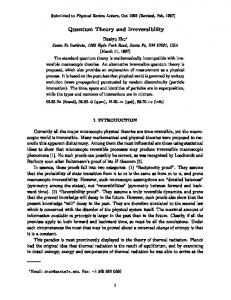
The behavior of F (t) = P(t), ML (t), MB (t), MD (t) or MT (t) averaged over initial states is qualitatively sketched in Fig. 1. A short-time transient is followed by an asymptotic decay and finally by saturation. The level of saturation is easily determined by ergodicity as N −1 , in terms of the Hilbert space size N , i.e. the number of states in a complete orthogonal basis of the system. In a cubic system in d dimensions, one has N = (L/ν)d , with ν the particle wavelength. The short-time transient is generically parabolic, as is easily obtained from short-time perturbation theory. Our interest in this review focuses on the intermediate, asymptotic decay regime, which lies between these two, somewhat trivial, regimes. For the sake of completeness, we nevertheless mention and sometimes briefly discuss
14
Figure 1 Sketch of the successive decay regimes of F (t) = P(t), M L (t), M B (t), M D (t) or M T (t) as a function of time. There is a short-time transient regime, well captured by first-order perturbation theory in time, followed by an asymptotic decay, and eventually by saturation at a value given by the inverse N −1 of the size of the considered Hilbert space / the effective Planck constant. The asymptotic decay is typically exponential or Gaussian in chaotic systems. In coupling regimes which are intermediate between first-order perturbation theory and golden rule regime, the decay can even be first exponential, then Gaussian (Cerruti and Tomsovic, 2002). In regular systems, the asymptotic decay is typically algebraic, and F (t) usually saturates above N −1 . This sketch corresponds to an average taken, e.g., over an ensemble of initial states. For a given initial states, fluctuations are observed, in particular, there is no long-time saturation, and instead one observes quantum revivals.
the other two regimes whenever needed. In the semiclassical limit, it turns out that the behavior of ML (t), MB (t) or MD (t) are closely related, and we therefore first focus this short survey of existing results on the Loschmidt echo. These results are summarized in Table II. We next briefly comment on the similarities and discrepancies between the Loschmidt echo and the purity, taken either as a measure of entanglement between two sub-systems of a bipartite systems, or as a measure of decoherence. At this point, we warn the reader that this survey by no means claims to be exhaustive. Our purpose here is to present a comprehensive table summarizing generic echo and purity behaviors. Accordingly, we deliberately omit exotic – but certainly interesting – behaviors occurring in specific situations, such ˇ as the fidelity freeze occurring for perturbations lacking first order contribution (Prosen and Znidariˇ c, 2005), or for specific choices of initial states (Weinstein et al., 2003), as well as parametric changes with time in the decay of ML in systems with diffractive impurities (Adamov et al., 2003), or in the crossover between two parametric regimes of perturbation (Cerruti and Tomsovic, 2002). What determines the asymptotic decay of ML ? Quite obviously, it should depend on the strength of Σ, and it was shown in Ref. (Jacquod et al., 2001) that the relevant measure for this strength is provided by the average golden rule spreading Γ = 2π|hα(0) |Σ|β (0) i|2 /δ of eigenstates α(0) of H0 over the eigenbasis {α} of H induced by the difference Σ = H − H0 . Different decay regimes are obtained depending on the balance of Γ with two additional energy scales (Jacquod et al., 2001): the energy bandwidth B of the unperturbed Hamiltonian H0 , and the level spacing δ = B~eff , with the effective Planck’s constant ~eff = ν d /Ω, given by the ratio of the wavelength volume to the system’s volume. Parametrically, these three regimes are (I) the weak perturbation regime, Γ < δ, (II) the golden rule regime, δ . Γ ≪ B, and (III) the strong perturbation regime, Γ > B. These three regimes are differentiated by the behavior of the local spectral density of perturbed states over the unperturbed ones – we come back to this below. In Ref. (Jacquod et al., 2001), the golden rule regime was first defined by bounds on the strength of the perturbation Σ for which the local density of eigenstates of H0 over the eigenstates of H acquires a Lorentzian shape. Accordingly, the Lyapunov decay ML (t) ∝ exp[−λt] to be discussed below occurs in the golden rule regime for the local spectral density of states.
15
Figure 2 Wavepacket evolution in a Lorentz gas. The initial wavepacket |ψ0 i is represented in the top left panel by a small dark spot. The large disks are fixed hard-wall scatterers. The top right and bottom left panel show |ψF i = exp[−iH0 t]|ψ0 i and |ψR i = exp[−iHt]|ψ0 i respectively. From the point of view of their spatial distribution, |ψF i and |ψR i look very similar, and one would naively expect 1 − M L (t) ≪ 1. This is not the case however, as the components of |ψF i are pseudo-randomly out of phase with respect to those of |ψR i. This results in a strong discrepancy between initial (top left) and final (bottom right panel) wavepackets whose scalar product gives f (t). (Figure taken from Ref. (Cucchietti et al., 2002b), with permission. Copyright (2002) by the American Physical Society. http://link.aps.org/doi/10.1103/PhysRevB.70.035311)
To understand the decays prevailing in these three regimes, we start by making the trivial, though somehow enlightening statement that the decay of ML is governed by the scalar product hψR |ψF i of two normalized wavefunctions |ψF i = exp[−iH0 t]|ψ0 i and |ψR i = exp[−iHt]|ψ0 i. The magnitude of this scalar product is determined by (i) the spatial overlap of the two wavefunctions – a classical quantity, not much different from the overlap of two Liouville distributions – and (ii) phase interferences between the two wavefunctions – a purely quantum mechanical effect. A decay of ML due to smaller and smaller spatial overlaps is easy to understand at the classical level already. Because Σ = H −H0 6= 0, both wavepackets visit different regions of space, and the overlap between these two regions decreases with time. This mechanism however sets in for a classically sizable perturbation Σ, in a sense that will be defined shortly. Weak perturbations do not sensibly reduce the spatial overlap of |ψF i and |ψR i, even on time scales where a significant decay of ML is observed. Instead, ML decays due to mechanism (ii) above, i.e. the fact that different components of |ψF i and |ψR i acquire uncorrelated phase differences generated by Σ. This mechanism is illustrated in Fig. 2. The spatial distribution of the initial state |ψ0 i is depicted in the top left panel, and the top right and bottom left panel show its time-evolution under H0 and H0 + Σ, respectively. Even though the spatial probability distributions |hr|ψF i|2 and |hr|ψR i|2 look almost identical – compare the wave patterns on the top right and bottom left panels – ML is significantly smaller than one because of phase randomization. This can be inferred from the very different initial and final probability cloud, |hr|ψ0 i|2 (top left) and |hr| exp[iHt] exp[−iH0 t]|ψ0 i|2 (bottom right). Strong perturbations on the other hand ergodize exp[iHt] exp[−iH0 t]|ψ0 i very fast, so that overlaps are not relevant either, in the sense that ML decays with time scales associated with the longitudinal flow, much shorter than the typical time scale λ of overlap decays. It turns out that overlaps of wavepackets only rarely determine the asymptotic
16 ML (t) 1 − σ02 t2 exp[−σ12 t2 ] exp[−Γt] exp[−λt] (t0 + t)−α exp[−B 2 t2 ] N −1
Regime of validity First method of derivation σ0−1
t≪ σ1 ≪ δ δ.Γ≪B λ>Γ δ.Γ≪B λB t→∞
RMT RMT
Semiclassics Semiclassics
ψ0
H0
Any Any Any
Any Any Any
Classically Chaotic meaningful Classically Regular meaningful Any Any Any Any
Table II Summary of the different decays and decay regimes for the average Loschmidt echo M L (t). The treatment of regular systems assumes that no selection rule exists for transitions induced by Σ. This might be hard to achieve in regular systems. Accordingly, the power-law decay in the table’s fifth row is to be taken with a grain of salt. The asymptotic saturation M L (∞) = N −1 at the inverse Hilbert space size is also based on the same assumption. If selection rules exist, M L saturates at a larger value. Exotic behaviors occurring in specific situations such as fidelity freeze (for phase-space displacements or perturbation without first-order contribution) have been deliberately omitted from this table. In this table, as in the rest of the article, actions are expressed in units of ~, which we accordingly set equal to one.
decay of the Loschmidt echo in quantum chaotic systems. It is in fact the rule rather than the exception that ML decays because of Σ−induced dephasing of |ψF i against |ψR i – we are obviously discussing relative dephasing due to the absence of Σ in the forward time-evolution. Additionally, wavefunction overlaps are relevant only for specific choices of classically meaningful ψ0 , such as narrow Gaussian wavepackets, or position states (Iomin, 2004; Jacquod et al., 2002; Jalabert and Pastawski, 2001; Vaniˇcek and Heller, 2003). When it is relevant, the overlap decay is very sensitive to the dynamics generated by the unperturbed Hamiltonian, but is mostly insensitive to Σ. Let us discuss this more quantitatively. The condition Γ < δ for the weak perturbation regime (I) legitimates the use of first-order perturbation theory in Σ, in which case the relative dephasing between |ψF i and |ψR i is weak and leads to a Gaussian decay ML (t) ≃ exp(−σ12 t2 ). The decay rate is given by σ12 ≡ hα(0) |Σ2 |α(0) i − hα(0) |Σ|α(0) i2 , averaged over the ensemble {α(0) } of eigenstates of H0 (Peres, 1984). The dephasing is of course strongest in the strong perturbation regime (III) where it generically leads to another asymptotic Gaussian decay ML (t) ≃ exp(−B 2 t2 ) (Jacquod et al., 2001) (perhaps excepting specific systems with pathological density of states). The intermediate golden rule regime (II) is of much interest, in that it witnesses the competition between overlap decay and dephasing decay. For classically chaotic systems, the decay of ML is exponential, ML (t) ≃ exp[−min(Γ, λ)t], with a rate set by the smallest of Γ – characterizing dephasing – and the system’s Lyapunov exponent λ > 0 – characterizing the decay of spatial overlaps (Jacquod et al., 2001). The physics behind this quantum–classical competition is that both overlap and dephasing mechanisms are simultaneously at work here and they both originate from explicitly separable contributions to ML . They are therefore additive. Because they both lead to exponential decays, the decay of ML is therefore governed by the slowest of the two. The situation is different in regular systems, where slightly perturbed wavepackets move away from unperturbed ones at an algebraic rather than exponential rate. Accordingly, one expects a power-law decay of ML (Jacquod et al., 2003) (see also Ref. (Emerson et al., 2002)). These results are summarized in Table II. The rough classification presented here is based on the scheme of Ref. (Jacquod et al., 2001) which relates the behavior of ML in quantum dynamical systems with smooth potentials to the Fourier transform of the local spectral density of eigenstates of H0 over the eigenbasis of H (Jacquod et al., 2001; Wisniacki and Cohen, 2002). Accordingly, regime (II) corresponds to the range of validity of Fermi’s golden rule, where the local spectral density has a Lorentzian shape (Frahm and M¨ uller-Groeling, 1995; Fyodorov and Mirlin, 1995; Jacquod and Shepelyansky, 1995; Jacquod et al., 2001; Wigner, 1955; Wisniacki and Cohen, 2002). A similar correspondence has been emphasized between the local spectral density of states and the return probability (Cohen and Heller, 2000). It should be stressed however that the Fourier transform of ML (t) would be equal to the local spectral density of states, in exactly the same way as the return probability, only if the initial state ψ0 were an eigenstate of H0 (or of H). The choice of ψ0 is largely irrelevant in the golden rule regime, but it is essential that ψ0 is classically meaningful (a narrow wavepacket or a position state) for a decay rate given by the Lyapunov exponent. Other investigations beyond this qualitative picture have focused on deviations from the behavior ∝ exp[−min(Γ, λ)t] in regime (II) due to action correlations in weakly chaotic systems (Wang, 2008; Wang et al., 2004, 2008). Quantum disordered systems with diffractive impurities (not with smooth potentials) have been predicted to
17 exhibit golden rule decay ∝ exp[−Γt] and Lyapunov decay ∝ exp[−λt] in different time intervals for otherwise fixed parameters (Adamov et al., 2003), while another crossover has been shown to occur between an exponential decay at short times and a Gaussian decay at long times in the crossover regime between (I) and (II) (Cerruti and Tomsovic, 2002). Let us finally mention Ref. (Garcia-Mata et al., 2003) which showed that, for open systems, the Lyapunov decay of ML (t)−ML (∞) is followed at times larger than the Ehrenfest time (to be defined below) by a decay governed by Ruelle-Pollicot resonances (Cvitanovi´c et al., 2005; Ruelle, 1986a,b). While certainly interesting from a mathematical point of view, this decay is barely noticeable in practice and we will not discuss it any further. Investigations of the dependence of ML on the choice of the initial state considered the Loschmidt echo for a prepared initial state ψT = exp[−iH0 T ]ψ0 obtained by evolving a Gaussian wavepacket ψ0 during a time T (Karkuszewski et al., 2002). One is then interested in the quantity MT (t) = |hψT | exp[iHt] exp[−iH0 t]|ψT i|2 = |hψ0 | exp[iH0 T ] exp[iHt] exp[−iH0 t] exp[−iH0 T ]|ψ0 i|2 .
(1.25)
The preparation time obviously does not lead to additional dephasing, and therefore the perturbation-dependent decay exp[−Γt] does not depend on T . However, the wavepacket spreads during the preparation, and therefore, the overlap of the two wavefunctions |ψF i = exp[−iH0 t] exp[−iH0 T ]|ψ0 i and |ψR i = exp[−iHt] exp[−iH0 T ]|ψ0 i picks up an additional dependence ∝ exp[−λT ], which turns the Lyapunov decay into ∝ exp[−λ(t + T )]. These results are discussed in Section II.E. They were first obtained in Ref. (Jacquod et al., 2002). The displacement echo MD (t) introduced in Eq. (1.23) is remarkable in that the perturbation does not lead to dephasing between otherwise unperturbed trajectories. In the regime δ . Γ ≪ B, MD (t) ∝ exp[−λt] only decays because the momentum displacement leads to the decrease of wavefunction overlaps. This is not the full story, however, as for small displacements, this overlap cannot decay to its minimal, ergodic value. In this case, the short-time (but still asymptotic) exponential decay with the Lyapunov exponent is followed by a quantum freeze at a displacementdependent value which can exceed the ergodic value N −1 by orders of magnitude if the displacement is small. It seems that the easiest way to observe direct manifestations of the classical Lyapunov exponent in quantum mechanics is the displacement echo. It is remarkable that, according to both trajectory–based semiclassics and RMT, the purity P(t) of the reduced density matrix in bipartite interacting dynamical systems exhibits the same phenomenology as ML , up to short-time discrepancies (Fujisaki et al., 2003; Jacquod, 2004a; Petitjean and Jacquod, 2006a; Tanaka et al., 2002), provided one replaces δ, B and Γ with two-particle level spacing and bandwidth δ2 and B2 and the interaction-induced golden rule broadening Γ2 of two-particle states. For P(t), the Lyapunov decay goes into the sum of two exponentials with both particle’s Lyapunov exponent, exp[−λt] → exp[−λ1 t] + exp[−λ2 t]. Mathematically speaking, the parallel behaviors of ML and P(t) come from the fact that both semiclassics and RMT rely on pairing – of either classical trajectories (motivated by a stationary phase approximation), or of wavefunction components (originating from the assumed RMT invariance of the distribution of eigenfunction components against basis transformation (Mehta, 1991)). This effectively leads to a decay of P(t) given by either dephasing generated by the coupling between particles, or the decay of overlaps of two initially identical wavefunctions evolving under two Hamiltonians differing by their coupling to a second particle with different initial conditions. After RMT pairing of wavefunction components or semiclassical pairing of classical paths, the mathematics of P(t) is mostly the same as that of ML (t). We now know that the purity P(t) and the Loschmidt echo ML (t) have essentially similar behaviors, in that the decays they exhibit are in a one-to-one correspondence. What about the Boltzmann echo ? Its definition, Eq. (1.15), puts it somehow in between P(t) and ML (t), one thus expects that it exhibits the same variety of decays. This is indeed the case, up to the important caveat that the rate of all perturbation dependent decays is given by the sum of a term depending on the accuracy with which the system is time-reversed and a term depending on the coupling between the two subsystems. Also, there is no dependence on the dynamics of the uncontrolled subsystem since the corresponding degrees of freedom are integrated out of the problem, and the symmetry exhibited by P(t) between the two subsystems is lost. With this we end this voluntarily short and nonexhaustive survey of previously obtained results. Before going into details of the derivation of these results, we give the outline of this review. E. Outline
In Section II, we discuss reversibility in quantum dynamical systems with few degrees of freedom. We focus on the Loschmidt echo, Eq. (1.1), and describe both the semiclassical and the RMT approaches in some details. This lays the foundation for the use of these analytical methods in later sections. Using these two methods of choice in this review, we calculate both the average fidelity and its mesoscopic fluctuations, computed over ensembles of spatially distinct, but structurally similar initial states. In the last two Chapters of Section II, the discussion digresses
18 somehow from ML towards the more specific, but experimentally relevant displacement echoes, for which we stress the connections and the differences with the standard Loschmidt echo. In Section III we revisit several aspects of the Loschmidt echo, this time following a phase-space approach. The approach is partially motivated by recent discussions on sub-Planck scale structures in the Wigner functions. Their existence is well established and certainly not put in doubt, however, we comment on whether they are relevant for understanding quantum reversibility and decoherence. While there is no observed behavior of the Loschmidt echo that cannot be explained by analytical realspace methods, our phase-space approach based on Wigner functions is very instructive in emphasizing the quantumclassical competition between the two sources of decay of ML – dephasing due to imperfect time-reversal and decay of overlap of initially identical wavepackets evolving with two different dynamics. It complements, and does not invalidate arguments relating dephasing to sub-Planck scale structures (Karkuszewski et al., 2002; Zurek, 2001). In Section IV we address the problem of how entanglement between two dynamical sub-systems is generated once they start to interact. Here, in some similarity with Section II, we witness a quantum-classical competition between coupling-induced and dynamically-induced generation of entanglement. In Section IV.F we discuss realistic reversibility experiments in presence of coupled uncontrolled degrees of freedom – the problem of the Boltzmann echo. There, the fidelity decay rate is bounded from below by the unavoidable generation of entanglement with the uncontrolled degrees of freedom. We argue that this might well have been observed experimentally in Ref. (Pastawski et al., 2000). Conclusions and final discussions are presented in Section V. II. IRREVERSIBILITY IN QUANTUM MECHANICS - THE LOSCHMIDT ECHO
Our aim in this chapter is to investigate quantum irreversibility in dynamical systems with few degrees of freedom by means of the fidelity of Eq. (1.1). We stress right away that, despite frequent claims to the contrary, our investigations have little – if anything – to do with the second law of thermodynamics, Boltzmann’s H-theorem, and the emergence of irreversibility in large systems with macroscopic numbers of interacting degrees of freedom. A probabilistic solution to the irreversibility paradox and the Boltzmann-Loschmidt controversy (Loschmidt, 1876) was already given in the late nineteenth century (Boltzmann, 1896) and, with certain refinements, still holds to this day (Lebowitz, 1999). The argument can straightforwardly be extended to quantum mechanics – both quantum and classical macroscopic systems become irreversible in essentially the same way (Lebowitz, 1999). The situation is however different for microscopic systems with few degrees of freedom. Simple mechanisms of irreversibility already exist at the microscopic level in chaotic classical systems with few degrees of freedom, where the properties of ergodicity and mixing ensure that, after a sufficiently long evolution, two initially well separated phase-space distributions evenly fill phase-space cells on an arbitrarily small scale (of course smaller scales require longer evolutions). Since phase-space points can never be located with infinite precision – one might think of unavoidable round-off errors in numerical simulations, external sources of noise or finite measurement resolution – irreversibility sets in after mixing has occurred on a scale smaller than the typical phase-space resolution scale. This mechanism cannot be carried over to quantum systems, however, mostly because the Schr¨odinger time-evolution is unitary, in either real- or momentum-space, and that a phasespace resolution on a scale comparable to Planck’s constant is sufficient (see however Section III for a discussion of sub-Planck scales in phase-space representations of quantum mechanics). The coarse-graining of phase-space that is effectively brought by unavoidable finite resolutions of the state of the system, and which is one of the two key ingredients of the just described scenario for classical irreversibility, is obviously less efficient in quantum systems – they are discrete by nature. Microscopic quantum systems are generically stable under time-reversal, even when their classical counterpart is irreversible (Shepelyansky, 1983). This picture is however incomplete. Peres, pointing out that quantum systems can never be considered isolated, suggested accordingly to investigate quantum irreversibility at the microscopic level through the fidelity [we rewrite Eq. (1.1)] ML (t) = |hψ0 |exp[iHt] exp[−iH0 t]| ψ0 i|2 ,
(2.1)
with which a quantum state ψ0 can be reconstructed by inverting the dynamics after a time t with a perturbed Hamiltonian H = H0 + Σ (Peres, 1984). Because of its connection with the gedanken time-reversal experiment proposed by Loschmidt in his argument against Boltzman’s H-theorem (Loschmidt, 1876), ML has been dubbed the Loschmidt echo by Jalabert and Pastawski (Jalabert and Pastawski, 2001), hence the subscript “L” in Eq. (2.1). The present section is concerned with the calculation of ML as a measure of reversibility for small quantum dynamical systems. We first present a semiclassical calculation, which we then compare to a RMT calculation. Our analytical predictions are next confirmed by numerical experiments. We finally investigate an offspring of the Loschmidt echo, the displacement echo defined above in Eq. (1.23).
19 A. Semiclassical approach to the Loschmidt echo
Semiclassical approaches have been successfully applied in various forms to the calculation of the fidelity (Cerruti and Tomsovic, 2002; Combescure, 2005; Combescure and Robert, 2007; Cucchietti et al., 2004; Jacquod et al., 2003; Jalabert and Pastawski, 2001; Petitjean and Jacquod, 2005; Vaniˇcek, 2004; Vaniˇcek and Heller, 2003; Wang et al., 2007, 2005; Wang and Li, 2005). It is probably fair to say that, while these works certainly amplified on Ref. (Jalabert and Pastawski, 2001) and improved it, they mostly only confirmed the most important result obtained there, that under certain circumstances, the quantum mechanical fidelity in chaotic dynamical systems decays at a rate determined by the classical Lyapunov exponent. The search for classical Lyapunov exponents in quantum mechanics is a celebrated problem in quantum chaos (Haake, 2001; Haake et al., 1992; Peres, 1993), and a significant part of the importance of Ref. (Jalabert and Pastawski, 2001) was to analytically predict that the decay of ML (t) can sometimes be governed by Lyapunov exponents. This is not the first occurrence, however, of a Lyapunov exponent in the time-evolution of a quantum system. Zurek and Paz (Zurek and Paz, 1994) predicted that the rate of increase of the von Neumann entropy S of an inverted Harmonic oscillator weakly coupled to a sufficiently warm heat bath would increase linearly with the rate λiho at which two neighboring trajectories move exponentially away from one another, ∂t S = λiho . They called λiho the system’s ”Lyapunov exponent”, though strictly speaking, the inverted harmonic oscillator is integrable with a vanishing Lyapunov exponent – its inverse parabolic potential generates sensitivity to initial conditions but no folding. They nevertheless made the leap of faith that, under the same conditions, chaotic dynamical systems with true positive Lyapunov exponent λ > 0 have ∂t S = λ. This is certainly not a trivial step, as truly chaotic systems not only exhibit local exponential instability, but stretching, contracting and folding of phase-space distributions, which certainly have an effect on wavepacket dynamics. Yet, Zurek and Paz’s prediction was later confirmed by Miller and Sarkar in their numerical analysis of the kicked rotator – a model that can be tuned to be truly chaotic – coupled to a bath of noninteracting harmonic oscillators (Miller and Sarkar, 1999a). The intuition gained in the study of the inverted oscillator seems to be valid, at least up to some extent. The question is still whether such occurrences of classical Lyapunov exponents in quantum mechanics require large heat bath, and if they are restricted to the high temperature regime, as suggested by subsequent refinements of the theory of Paz and Zurek. Perhaps more importantly, can one analytically investigate quantal systems with a well-defined, truly chaotic limit – in the mathematically rigorous definition discussed above – and predict the emergence of a Lyapunov-driven behavior of some of its properties in a well-defined regime of parameters ? Jalabert and Pastawski gave a positive answer to the first part of that question, but only specified that their approach is valid for a quantum mechanically large, but classically weak perturbation. They made no comment on what this quantitatively means. That second, equally important part of the question was answered by Jacquod, Silvestrov and Beenakker (Jacquod et al., 2001) who obtained precise parametric bounds and quantitative estimates for the validity of the theory of Ref. (Jalabert and Pastawski, 2001) from a comparison of semiclassics with RMT. To make a long story short, Ref. (Jacquod et al., 2001) argued that, first, in a regime to be determined, the decay of ML is given by the sum of the two semiclassical decays ∝ exp[−Γt] + exp[−λt], both terms being multiplied by prefactors of order one. This implicitly follows from the calculation of Ref. (Jalabert and Pastawski, 2001), but was not explicitly stated there. Second, by analogy with RMT, which relates the decay of ML with the Fourier transform of the local density of states – the energy-resolved projection of eigenstates of H0 over the basis of eigenstates of H – the decay term ∝ exp[−Γt] was predicted to occur whenever the local spectral density of states is Lorentzian. Ref. (Jacquod et al., 2001) concluded that the regime of validity of Ref. (Jalabert and Pastawski, 2001) is defined by the regime of perturbation leading to a Lorentzian local density of states. A RMT approach identified this regime as δ . Γ ≪ B in Ref. (Frahm and M¨ uller-Groeling, 1995; Fyodorov and Mirlin, 1995; Jacquod and Shepelyansky, 1995), based on rather general grounds. It thus appears that quantum mechanically large means that the perturbation broadens eigenstates to an energy width larger than the level spacing, thereby making the spectrum effectively continuous, while classically weak means that this broadening must be much smaller than the system’s bandwidth. When these two conditions are met, the above argument predicts ML ∝ exp[−min(Γ, λ)t]. Looking back, these statements and this line of reasoning sound almost trivial. It is therefore important to recall that the range of applicability of the semiclassical theory of ML was not known before Ref. (Jacquod et al., 2001). Semiclassical methods apply to the case of classically relevant initial states ψ0 , such as the narrow Gaussian phasespace wavepackets considered in this chapter. Real-space semiclassics also relies on stationary phase approximations, which implicitly assumes that enough action phase has been accumulated on the considered classical trajectories, and for times at least shorter than the time it takes to resolve the discreteness of the quantum spectrum – beyond that, purely quantum effects set in which are not captured by semiclassics. These points, which we rephrase more quantitatively below, have to be kept in mind – the method presented in this section applies to the regime of asymptotic decay and of saturation of ML , but not to the short-time initial transient regime. Additionally, as just mentioned, the perturbation Σ has to be quantum-mechanically large – semiclassics as presented in this chapter does not apply to the first-order perturbation regime – but classically small. The semiclassical results to be presented in this chapter
20 thus are not valid outside the regime defined by δ . Γ ≪ B (Jacquod et al., 2001). These gaps in the theory will be filled in the next section on RMT. Here we extend the work of Jalabert and Pastawski (Jalabert and Pastawski, 2001) beyond the special case of an extended impurity perturbation potential. It was indeed pointed out in Ref. (Jacquod et al., 2003) (but probably known to the authors of Ref. (Jalabert and Pastawski, 2001)) that only bounds on the decay in time of classical correlators matter in the semiclassical calculation of ML – at least up to a phenomenological constant which eventually can be related to the golden rule spreading Γ (Cerruti and Tomsovic, 2002; Jacquod et al., 2001). The semiclassical calculation of the average Loschmidt echo has already been described in great details in several publications, therefore we only repeat the steps that are required to make this section self-consistent. 1. Ensemble average
The semiclassical approach to the Loschmidt echo requires that the initial state is classically meaningful, that it is either a position state or a narrow wavepacket in phase-space. Semiclassics can also be extended to coherent or incoherent superpositions of such states, provided one can neglect the mutual overlap of the different states in the superposition. In this chapter, we consider an initial narrow Gaussian wavepacket ψ0 (r′0 ) = (πν 2 )−d/4 exp[ip0 · (r′0 − r0 ) − |r′0 − r0 |2 /2ν 2 ] in d dimensions. To time-evolve it, we use the semiclassical approximation for the time-evolution kernel discussed in Appendix A (Cvitanovi´c et al., 2005; Gutzwiller, 1990; Haake, 2001) Z X hr| exp(−iH0 t)|ψ0 i = dr′0 (2.2a) KsH0 (r, r′0 ; t)ψ0 (r′0 ), s
KsH0 (r, r′0 ; t) =
1/2 Cs (2πi)d/2
exp[iSsH0 (r, r′0 ; t) − iπµs /2].
(2.2b)
The semiclassical propagator KsH0 (r, r′0 ; t) is expressed as a sum over classical trajectories (labeled s) connecting r and r′0 in the time t. For each s, the partial propagator contains the action integral SsH0 (r, r′0 ; t) along s, a Maslov index µs , and the determinant Cs of the stability matrix. Once this time-evolution is inserted into expressions involving more than one time-evolution operator, quantum coherent effects can be captured via nontrivial phase interferences involving two or more classical trajectories with different action phases. In the cases investigated in this review, such nontrivial effects already occur at the level of diagonal pairing, setting classical trajectories pairwise equal to one another, where one element of the pair feels the effect of the perturbation (corresponds to H) while the other one does not (as it corresponds to H0 ). What is the range of validity of the semiclassical approach ? To answer this question, one needs to discuss the hierarchy of important time scales we consider in this review in some more details. The semiclassical propagator, Eq. (2.2b), is derived from the Feynman-Kac path integral expression for the quantum time-evolution operator, once a stationary phase condition is enforced. The latter requires that the action phase accumulated on almost all paths in the path integral (not only the classical ones) is much larger than 1 (in units of ~). This requires a minimal time which can be estimated as τmin = 1/E, with the energy E of the system. For larger times, the Hamiltonian flow generates enough action phase to justify a stationary phase condition. The approach also breaks down at longer times, and certainly loses its validity once the discreteness of the spectrum is resolved, i.e. for times longer than the Heisenberg time τH = ~/δ with the level spacing δ of the system considered. (This time is determined by a standard uncertainty relation with the level spacing, hence its name.) Earlier breakdowns can occur due to the proliferation of conjugate points, and it has been numerically observed that the semiclassical approach permits to calculate the time evolution of smooth, initially localized wavepackets with a reasonable accuracy up to algebraically long times in the effective Planck’s constant ∝ O(~−a eff ) (with a > 0) (Heller and Tomsovic, 1993; Tomsovic and Heller, 1991). The semiclassical methods employed in this review are not applicable outside the time interval [τmin , τH ]. This interval is parametrically very large in ~eff in the semiclassical limit. Beside these two quantum time scales, classical time scales limit the applicability of our approach in that they give bounds for some statistical assumptions we have to make as we go along. Closed chaotic systems are characterized first by the time of flight τf = L/v, i.e. the time it takes to cross the system once. This time is however so small – the velocity of the particle becoming larger and large in the semiclassical limit – that we neglect it altogether and set it equal to zero. A second important classical time scale is the Lyapunov time λ−1 , roughly giving the time it takes for local exponential instability to set in. Next one has the ergodic time τerg measuring the time it takes for an initial condition to have visited most of its available phase-space. This time scale is also assumed to be very short. Still one has to keep in mind that the sum rules we employ are often justified by ergodicity assumptions which break down at times shorter than τerg . There remains one important quantal time scale to discuss, and it is the Ehrenfest time
21
Figure 3 Diagrammatic representation of the average fidelity M L and the trajectory pairings leading to the Lyapunov decay ∝ exp[−λt] (for chaotic systems – for regular ones this contribution gives an algebraic decay), the golden rule decay ∝ exp[−Γt] and the long-time saturation of M L . The semiclassical fidelity is expressed as a four-fold sum over unperturbed (solid lines) and perturbed (dashed lines) classical trajectories (left-hand side). This sum is reduced to single and double sums after semiclassically motivated stationary phase conditions are enforced (right-hand side). The exponential decay with the Lyapunov exponent (first term on the right-hand side) goes into an algebraic decay for regular systems (see Table II).
τE = λ−1 ln L/ν. This time is logarithmic in ~eff = ν/L, is always much shorter than τH in the semiclassical limit, and gives bound for the onset of coherence effects in semiclassics. In summary, our semiclassical approach is valid in a parametrically large regime of time, bounded from below by either a classical ergodic time or the time it takes to accumulate enough action phase to justify stationary phase approximations, and bounded from above by a time algebraically large in ~eff , which is smaller or equal to the Heisenberg time it takes to resolve the discreteness of the underlying quantum spectrum. Within the semiclassical approximation the fidelity reads, not so elegantly, Z Z Z X ML (t) = dr dr01 dr02 ψ0 (r01 )ψ0∗ (r02 ) KsH10 (r, r01 ; t) [KsH2 (r, r02 ; t)]∗ s1 ,s2
×
Z
dr′
Z
dr′01
Z
dr′02 ψ0∗ (r′01 )ψ0 (r′02 )
X
[KsH30 (r′ , r′01 ; t)]∗ KsH4 (r′ , r′02 ; t) .
(2.3)
s3 ,s4
This expression is easily obtained by inserting four semiclassical time-evolution kernels, Eq. (2.2), into Eq (2.1). The fidelity is given by a six-fold integral over initial and intermediate (at time-reversal) positions, with additionally a fourfold sum over classical trajectories. To reduce this to a useful, tractable expression, one first notices that because ψ0 is a narrow Gaussian wavepacket centered on r0 , one can linearize the integrand in r0i = r0 + δr0i and r′0i = r0 + δr′0i , then perform the resulting (Gaussian) integrals over initial positions. The second step is to enforce semiclassically motivated stationary phase conditions that reduce the four-fold sum over classical paths to three dominant terms, two involving a two-fold sum, one involving a single sum over classical paths. The structure of the semiclassical approximation to the average fidelity at this stage is sketched on the right-hand side of Fig. 3. Classical trajectories are represented by a full line if they correspond to H0 and a dashed line for H, with an arrow indicating the direction of propagation. For a given initial condition r0 , each contribution consists in four classical paths connecting r0 to two final evolution points r and r′ . The motivation for enforcing a stationary phase condition on the action phase differences Ss1 (r, r0 ; t) − Ss2 (r, r0 ; t) and Ss3 (r, r0 ; t) − Ss4 (r, r0 ; t) appearing in Eq. (2.3) – the phases are contained in the partial semicassical propagators Ks , see Eq. (2.2) – is that we calculate the fidelity averaged over an ensemble of initial Gaussian wavepackets ψ0 . As the center of mass r0 of these initial states is moved, the phase differences fluctuate, so that the only contributions that survive the average are those which minimize these fluctuations. The dominant such contribution is obtained from the diagonal approximation s1 = s2 , s3 = s4 . But how can this be justified, given that s1,3 are classical trajectories generated by H0 , while s2,4 correspond to a different Hamiltonian H = H0 + Σ ? The answer is that setting s1 = s2 for two trajectories generated by two different chaotic Hamiltonians H = H0 + Σ is justified by shadowing and the structural stability of hyperbolic systems for not too large Σ (Katok and Hasselblatt, 1996). In the context of the fidelity, this point was first mentioned in Refs. (Cerruti and Tomsovic, 2002; Vaniˇcek and Heller, 2003), and we discuss it further below in Chapter II.E. Here we only mention what this qualitatively means. Structural stability/shadowing theorems state that almost all trajectories of slightly perturbed classical hyperbolic systems come in a one-to-one correspondence with the trajectories of the corresponding unperturbed hyperbolic system, in that for each unperturbed trajectory, there exists a perturbed trajectory which remains in its immediate vicinity. The two
22 trajectories do not share endpoints in general, but it does not matter for our purpose here, all we need being that they stay a distance less than the quantum mechanical resolution apart. Setting s1 = s2 thus means that we chose s2 to be the shadow of s1 . While strictly speaking shadowing and structural stability theorems apply to uniformly hyperbolic systems only, numerical investigations have shown that generic chaotic systems also display structural stability and shadowing of trajectories upon not too strong perturbations (Grebogi et al., 1990). Therefore, setting s1 = s2 is justified for chaotic systems. There is no such principle that justifies setting the diagonal pairing of trajectories in regular or integrable systems, however, and, despite several convincing numerical confirmations, the results on regular systems to be presented below must be considered cautiously. Sort of ironically, the calculation to be presented is more reliable for chaotic than regular systems. But this makes a lot of sense, given that universality applies to chaotic systems, not to regular ones, which typically exhibit largely fluctuating system-dependent behaviors. After the linearization around r0 and this first stationary phase approximation, ML (t) is reduced to a double sum over classical paths s and s′ and a double integration over coordinates r and r′ , Z Z X ML (t) = (ν 2 /π)d dr dr′ Cs Cs′ exp[iδSs (r, r0 ; t) − iδSs′ (r′ , r0 ; t)] s,s′
× exp(−ν 2 |ps − p0 |2 − ν 2 |ps′ − p0 |2 ),
(2.4)
with δSs (r, r0 ; t) = SsH (r, r0 ; t) − SsH0 (r, r0 ; t). Our strategy next is to differentiate between contributions in Eq (2.4) where the trajectories s and s′ are correlated (s ≃ s′ , within a spatial resolution ν) from those where they are not. We call the correlated contribution the diagonal contribution, and the uncorrelated one the nondiagonal contribution by some abuse of language, even though both contributions already emerge from the diagonal approximation s1 ≈ s2 we made to go from Eq. (2.3) to Eq. (2.4). These two sets of contributions are quite different in essence, and they lead to fundamentally different decays. We argue in Appendix A that the decay of the diagonal contribution is governed by the decay of the overlap of |ψF i = exp[−iH0 t]|ψ0 i with |ψR i = exp[−iHt]|ψ0 i, while the behavior of the nondiagonal contribution is determined by the Σ-induced dephasing between the wavepacket propagating along s and the one propagating along s′ . Consequently, the diagonal contribution have a classical decay determined by the disappearance of wavefunction overlap. The latter occurs exponentially fast in chaotic systems, due to their characteristic exponential instability of neighboring orbits, but is much slower, it is in fact algebraic, in regular systems. Simultaneously, the decay of the nondiagonal contributions is governed by perturbation-generated dephasing between the forward and backward propagation along s and s′ . Because we neglected the effect of the perturbation on the classical trajectories – an approximation that was justified by invoking structural stability and shadowing – this dephasing is of purely quantal nature. It typically leads to an exponential decay in chaotic systems, and to a Gaussian decay in regular systems which often have surviving correlations. The Gaussian decay is however often masked because in regular systems, the diagonal contribution generates a much slower algebraic decay. We also note that the diagonal contribution sensitively depends on whether H0 is regular or chaotic, while the nondiagonal contribution is generically insensitive to the nature of the classical dynamics set by H0 , provided that the perturbation Hamiltonian Σ induces enough mixing of eigenstates of H0 , and in particular that it has no common integral of motion with H0 . In addition, there is a third contribution depicted in Fig. 3 which corresponds to the long-time saturation of ML (t). We seem to be the first to notice that the latter can also be calculated semiclassically. To see this, one has to go back one step before the diagonal approximation leading to Eq. (2.4). After one performs the linearization around r0 on Eq (2.3), one has Z Z X 2 d ML (t) = (ν /π) KsH10 (r, r0 ; t)[KsH2 (r, r0 ; t)]∗ [KsH30 (r′ , r0 ; t)]∗ KsH4 (r′ , r0 ; t) dr dr′ s1 ,s2 ,s3 ,s4
� � � × exp − ν 2 |ps1 − p0 |2 + |ps2 − p0 |2 + |ps3 − p0 |2 + |ps4 − p0 |2 /2 .
(2.5)
Pairing the trajectories as s1 = s3 and s2 = s4 cancels exactly all action phases. On the negative side, this pairing simultaneously requires r ≃ r′ within the wavelength resolution ν, a restriction that results in a reduction of its contribution by a prefactor ~eff . The calculation of this term is described in Appendix A, and we do not repeat it here. One gets a time-independent contribution ML (∞) = ~eff Θ(t > τE ),
(2.6)
corresponding to the long-time saturation of ML . This term requires that uncorrelated paths exist between r0 and r ≃ r′ (see the rightmost contribution sketched in Fig. 3) and therefore does not exist for times shorter than the Ehrenfest time τE ≡ λ−1 | ln[~eff ]|.
23 With all this we write (d)
(nd)
ML (t) = ML (t) + ML
(t) + ML (∞).
(2.7)
The trajectory pairings that lead to these three terms are summarized in Fig. 3. The above splitting of ML (t) into three terms is not only mathematically convenient, it is physically meaningful. The first term is phase-independent and we are momentarily going to argue that it decays with the decay of the overlap of ψ0 evolving under H0 with itself, when it is evolved under H = H0 + Σ. It is of purely classical origin – this is generic of semiclassically computed terms of maximal diagonal pairing (another example is the Drude conductance in the semiclassical theory of transport (Baranger et al., 1991)). The second term is perturbation-dependent and within the semiclassical approach, it decays with the variance of the phase difference accumulated along paired trajectories due to the presence of the perturbation. Strictly speaking, it is also a diagonal contribution. Its quantumness, however, originates in that the perturbation Σ affects the action phase accumulated along only one of the trajectories. In other words, dephasing due to Σ is taken into account. The third contribution finally corresponds to the unbreakable, time-independent, ergodic core of ML (t), i.e. that part which correspond to minimal overlap of two random, ergodic wavefunctions. On average they are not orthogonal (this would require a degree of correlation which gets lost in the long time evolution under two different Hamiltonians) and this is why ML (t) saturates at a finite value inversely proportional to the Hilbert space volume. Let us have a quick look at these decays and their origin in some more details. The calculation of all these contributions is presented in Appendix A. The decay of the nondiagonal contribution is governed by the action phases accumulated on the uncorrelated paths s 6= s′ . It is thus legitimate to perform the phase averaging separately for s and s′ with � � Z t Z t 2 ′ ′ 1 1 ˜ ˜ ˜ ˜ hexp[iδSs ]i = exp(− 2 hδSs i) = exp − 2 dt dt hΣ[q(t)]Σ[q(t )]i . (2.8) 0
0
Here q(t˜) lies on path s with q(0) = r0 and q(t) = r. In Ref. (Jalabert and Pastawski, 2001), a specific assumption was made about the perturbation potential, that it corresponds to a random distribution of extended impurities. This gives an exponential decay of the correlator in Eq. (2.8). Here we go beyond this approach, noting that, for chaotic systems, one generically observes fast decays of correlations. Under the assumption that Σ and H0 have no common integral of motion, so that δSs fluctuates fast and randomly enough, the correlator of Σ decays fast with time, which gives the golden rule decay Z Z 1 t ˜ t ˜′ (nd) dt dt hΣ[q(t˜)] Σ[q(t˜′ )]i, (2.9) ML (t) ∝ exp(−Γt), with Γt ≡ 2 0 0 regardless of whether H0 is chaotic or regular. This conclusion, that the golden rule decay holds whether H0 is regular or chaotic, can also be obtained via a fully quantum mechanical approach based on random-matrix theory assumptions for Σ, in which case the invariance under unitary transformations of the distribution of Σ is sufficient to (nd) obtain the exponential decay ML (t) ∝ exp(−Γt), irrespective of the distribution of H0 . However it has to be noted that the whole argument relies on the assumption that the perturbation correlator in Eq. (2.9) decays faster than t−1 , also in regular systems. While perturbations can be tailored to meet this assumption, there are certainly cases where the correlator oscillates in time or even saturates at a finite, nonzero value at large times. Several instances have been recorded where the decay of ML (t) in regular systems is Gaussian rather than exponential (Gorin et al., ˇ 2006; Prosen et al., 2003; Prosen and Znidariˇ c, 2002). This might reflect the nondecaying behavior of the correlator of Σ, but also indicates that the diagonal contributions do not exist, presumably because of lack of shadowing of unperturbed classical orbits by classical ones, i.e. the double diagonal approximation is not justified there. The calculation of the diagonal contribution is detailed in Appendix A.2. With Eqs. (A8), (A9), (A10), and (A11), Eq. (2.4) gives for the diagonal contribution to the Loschmidt echo Z Z X � 1 (d) 2 d ML (t) = (ν /π) dr+ dr− Cs2 exp − U τ r2− exp(−2ν 2 |ps − p0 |2 ), (2.10) 2 s with τ = t/6 for regular systems and τ = λ−1 (1 − exp[−λt]) ≃ λ−1 for chaotic systems, and U is defined in Eq. (A11) from the correlator of derivative of Σ, h∂i Σ[q(t˜)]∂j Σ[q(t˜′ )]i = U δij δ(t˜ − t˜′ ).
(2.11)
The rest of the calculation is straightforward. The Gaussian integration over r− ≡ r − r′ ensures that r ≈ r′ , and hence r+ ≡ (r + r′ )/2 ≈ r. One further uses one Cs (which is the determinant of a Jacobian) to perform a change
24 of variables from r+ to ps . For the remaining Cs we take into account the algebraic stability of regular systems with Cs ∝ t−d (regularized at short times with t0 ) to be contrasted with the exponential instability of chaotic systems with Cs ∝ exp[−λt]. One finally arrives at regular systems with U τ < ν −2 , t−d , (d) −3d/2 ML (t) ∝ (2.12) t , regular systems with U τ > ν −2 , exp[−λt], chaotic systems.
These decays are rather insensitive to the choice (A11) of a δ-function force correlator. Even a power-law decaying correlator ∝ |t˜ − t˜′ |−a reproduces Eqs. (2.12) at large enough times, provided a ≥ 1. These diagonal decays make a lot of sense, they actually agree rather well with our intuition, based on decays of overlaps of classical phasespace distributions. Translating the perturbation – which is assumed to be classically small – into slight phase-space displacements, one expects that the local exponential instability of chaotic systems leads to an exponential decay of these overlaps – this is confirmed by works on the classical fidelity, at least in some regime (Benenti and Casati, 2002; ˇ Benenti et al., 2003a,b; Eckhardt, 2003; Prosen and Znidariˇ c, 2002). Our semiclassical approach thus predicts that, up to the long-time saturation at the effective Planck’s constant, the Loschmidt echo is given by the sum of the diagonal and nondiagonal terms, t−d , regular systems with U τ < ν −2 , (nd) (d) −3d/2 ML (t) = ML (t) + ML (t) ∝ (2.13) t , regular systems with U τ > ν −2 , αe−λt + e−Γt , chaotic systems.
These results are valid in the asymptotic regime, past the initial parabolic transient (see Fig. 1), and as such they lose their validity at short times – Eqs. (2.13) does not predict a singularity at t = 0 for regular systems, nor ML (t = 0) = 1 + α > 1 for chaotic systems ! The predicted decays are parametric in essence, and are smoothly connected to the initial, short-time transient decay via weakly time-dependent prefactors of order one. This is confirmed by numerical works. It has to be kept in mind that the results given in Eq.(2.13) are averages over an ensemble of initial Gaussian wavepackets ψ0 . This is required to justify the semiclassical stationary phase approximations from which these results derive. Still the dominant, diagonal contribution to the fidelity for regular systems has been derived under the assumption that correlations decay fast enough, Eq. (A11). This is not always satisfied in regular systems, where it is actually the rule, rather than the exception, that correlators such as the one in Eq. (A11) decay more slowly than t−1 , i.e. a < 1. Assuming a constant correlator h∂i Σ[q(t˜)]∂j Σ[q(t˜′ )]i = U ′ δij
(2.14)
results in τ = t2 /8 in Eq. (2.10), which leads for U ′ t2 /8 > ν −2 to an accelerated, but still power-law decay of the diagonal contribution to the fidelity, ML (t) ∝ t−2d , in regular systems. We believe that the decay of the average fidelity in regular systems is generically algebraic, however, the exponent with which ML (t) decays can vary from case to case. It is well possible that the fidelity calculated for individual ψ0 exhibits different behaviors, as the Gaussian ˇ ones reported in Refs. (Gorin et al., 2006; Prosen et al., 2003; Prosen and Znidariˇ c, 2002), since it is an average over an ensemble of ψ0 that effectively leads to the integral over r− in Eq. (A12). Without that integration, one has a Gaussian time-dependence. (nd) In both regular and chaotic systems, the decay of ML (t) reflects the stability of nearby orbits, Cs ∝ exp[−λt] −d for chaotic, Cs ∝ t for regular systems. This is not the full story in regular systems, however, where the correlator (A11) contributes another t−d/2 for U t/6 > ν −2 , or t−d for U ′ t2 /8 > ν −2 . Compared to the “classical fidelity”, i.e. the overlap of classical phase-space distributions (Benenti and Casati, 2002; Benenti et al., 2003a,b; Eckhardt, ˇ 2003; Prosen and Znidariˇ c, 2002), the quantum fidelity decays faster in regular systems, because dephasing does not totally decouple from overlap. The same effect also occurs in chaotic systems where, however, it gives a subdominant, algebraic correction to the exponential Lyapunov decay of overlaps. This is hardly noticeable. Given the respective specificities of classical and quantum mechanical dynamics, and the structure of their equations of motion, it is at first glance quite surprising to observe Lyapunov exponents in the dynamics of quantal systems as directly as in the decay of the Loschmidt echo. The semiclassical approach presented above is however transparent enough that one can trace back the origin of the Lyapunov decay to the stability of chaotic classical trajectories. One concludes that the fidelity decays exponentially at the Lyapunov rate in precisely the same way as the overlap of two classical phase-space distributions, initially identical, but evolving under the influence of two slightly different Hamiltonians. Wisdom comes with experience and once this mathematical observation is done, having a Lyapunov
25 r2 s4
s3 s2
s7 r0
r3 s8
r1 s1
s5
s6 r4
Figure 4 Diagrammatic representation of the squared fidelity M 2L (t). (Figure taken from Ref. (Petitjean and Jacquod, 2005). Copyright (2005) by the American Physical Society.)
decay does not come as a surprise after all. But this is only one side of the story, which in particular neglects the second contribution to the Loschmidt echo, the one we called nondiagonal and which carries quantum coherence. In chaotic systems, we have seen that diagonal and nondiagonal contributions decay exponentially with time, so that their sum decays effectively with the weakest of the two decay rates, ML (t) ∝ exp[−min(Γ, λ) t]. This a very simple formula, which initially looked too simple to be true, even to two of the authors of Ref. (Jacquod et al., 2001) where it first appeared. It actually contains a lot more physics than meets the eyes at first glance. Most of all, it states that quantum mechanically strong, but classically weak perturbations can generate a decay of ML (t) which is totally governed by dephasing. There is thus a parametrically large regime where external perturbations have no observable classical dynamical effect, yet lead to the decay of the Loschmidt echo. In that regime, the handwaving argument, that ML (t) decays because the perturbation first leads to a small phase-space displacement which is subsequently exponentially amplified by the underlying classical dynamics is incorrect. It neglects the fact that pairing of trajectories is still possible between two slightly different Hamiltonian. This is the second surprise, and this time it remains a surprise even retroactively! It is concepts so deeply rooted into classical dynamics as shadowing and structural stability that allow dephasing to occur so fast that the perturbation at its origin has effectively no dynamical effect. In that regime, dephasing or decoherence cannot be apprehended by paradigms based on phase-space displacements. 2. Mesoscopic fluctuations
Fluctuations of a physical quantity often contain more information than its average. For example, quantum signatures of classical chaos are absent of the average density of states, but strongly affect spectral fluctuations (Haake, 2001). Here, we investigate the fluctuations of the Loschmidt echo as the initial state is modified. We will see that Lyapunov exponents can be extracted from the fluctuations of ML over a larger range of parameters than from the average of ML . However no fundamentally new physics emerges from fluctuations. Ref. (Silvestrov et al., 2003) presents the first investigation of the properties of ML beyond its average. It shows that, for classically large perturbations, Γ ≫ B, ML is dominated by very few exceptional events, so that the fidelity for a typical initial state is better described by exp[ln(ML )], and that ML does not fluctuate for times longer than the Ehrenfest time. Ref. (Petitjean and Jacquod, 2005) showed however that these conclusions do not apply to the regime of classically weak but quantum-mechanically strong perturbation, instead they are valid when the perturbation is classically large. In that regime, ML (t) measures what can still be successfully recovered after a hopelessly imperfect time-reversal operation is performed. Accordingly, ref. (Silvestrov et al., 2003) states that some recovery is possible if the time-reversal operation is performed soon enough that the perturbation has no time to propagate ergodically. Some numerical data for the distribution of ML in the weak perturbation regime were presented in Ref. (Gorin et al., 2004). Here, we focus on chaotic systems – we discuss only very briefly fluctuations of ML in regular or integrable systems at the end of this section – and investigate the behavior of the variance σ 2 (ML ) of the fidelity in the golden rule regime from a semiclassical point of view. We want to calculate M2L . Squaring Eq. (2.3), we see that it is given by eight sums over classical paths and twelve spatial integrations. We use the same tricks as for the average fidelity, first that spatial integrations over initial wavefunction coordinates can be brought to Gaussian form after the corresponding integrands have been linearized around r0 – eight of the twelve spatial integrals can be calculated in this way – and second to identify stationary
26 ≃
r2
r1 ≃ r3
r2 ≃ r4
r1
r3 r0
r1 ≃ r3
r2
2 r0
r0
r4
r4 α2 e−2λt
r2 ≃ r4
r1 ≃ r3
r2
2
r0 σ 2 (ML )
r1 ≃ r3
2αe−λt e−Γt
r4
2~eff e−Γt Θ(t − τE )
r0 ~2eff Θ(t − τE )
Figure 5 Diagrammatic representation of the averaged fidelity variance σ 2 (M L ) and the three time-dependent contributions that dominate semiclassically, together with the contribution giving the long-time saturation of σ 2 (M L ). There is no exp[−2Γt]-term. (Figure taken from Ref. (Petitjean and Jacquod, 2005). Copyright (2005) by the American Physical Society.)
phase solutions justified by our averaging over r0 . The starting point is M2L (t)
=
Z Y 4
drj
j=1
8 X
exp[i(Φ
si ;i=1
H0
H
− Φ − πΞ/2)]
Y
Cs1/2 i
i
�
ν2 π
�d/4
exp(−ν 2 δp2si /2).
(2.15)
P3 Here we introduced the staggered sum Ξ = i=0 (−1)i (µs2i+1 −µs2i+2 ) of Maslov indices and the momentum difference δpsi = psi − p0 . The right-hand side of Eq. (2.15) is schematically described in Fig. 4, where, as before, classical trajectories are represented by a full line if they correspond to H0 and a dashed line for H, with an arrow indicating the direction of propagation. In the semiclassical limit Ss ≫ 1 (we recall that actions are expressed in units of ~), and upon average over ψ0 , Eq. (2.15) is dominated by terms which satisfy a stationary phase condition, i.e. where the variation of the two differences of action phases ΦH0 = SsH10 (r1 , r0 ; t) − SsH30 (r2 , r0 ; t) + SsH50 (r4 , r0 ; t) − SsH70 (r3 , r0 ; t), Φ
H
=
SsH2 (r1 , r0 ; t)
−
SsH4 (r2 , r0 ; t)
+
SsH6 (r4 , r0 ; t)
−
SsH8 (r3 , r0 ; t),
(2.16a) (2.16b)
has to be minimized. These stationary phase terms are easily identified from the diagrammatic representation as those where two classical trajectories s and s′ of opposite direction of propagation are contracted, i.e. s ≃ s′ , up to a quantum resolution given by the wavelength ν. As mentioned above, contracting s (generated by H0 ) with s′ (generated by H = H0 + Σ) is justified by the structural stability of hyperbolic systems for not too large Σ (Katok and Hasselblatt, 1996). Paths contractions are represented in Fig. 5 by bringing two lines together in parallel. Contracting either two dashed or two full lines allows for an almost exact cancellation of the actions, hence an almost perturbationindependent contribution, up to a contribution arising from the finite resolution ν with which the two paths overlap. However when a full line is contracted with a dashed line, the resulting contribution still depends on the action R δSs = − s Σ(q(t), t) accumulated by the perturbation along the classical path s, spatially parametrized as q(t). Since we are interested in the variance σ 2 (ML ) = hM2L i − hML i2 (this is indicated by brackets in Fig. 5) we must subtract the nonconnected terms contained in hM2L i, i.e. those corresponding to independent contractions in each of the two subsets (s1 , s2 , s3 , s4 ) and (s5 , s6 , s7 , s8 ). The result is that all contributions to σ 2 (ML ) require pairing of spatial coordinates, |ri − rj | ≤ ν, for at least one pair of indices i, j = 1, 2, 3, 4 – in particular, this has the consequence that there is no exp[−2Γt]-term. With these considerations, the four dominant contributions to the fidelity variance are depicted on the right-hand side of Fig. 5. We calculate them one by one in Appendix A.3. The first one corresponds to s1 = s2 ≃ s7 = s8 and s3 = s4 ≃ s5 = s6 , which requires r1 ≃ r3 , r2 ≃ r4 , it gives a contribution σ12 = α2 exp[−2λt],
(2.17a)
where α is the same as in Eq. (2.13). The second dominant term is obtained from s1 = s2 ≃ s7 = s8 , s3 = s4 and s5 = s6 , with r1 ≃ r3 , or equivalently s1 = s2 , s7 = s8 and s3 = s4 ≃ s5 = s6 with r2 ≃ r4 . This term comes therefore with a multiplicity of two, and one obtains σ22 ≃ 2α exp[−λt] exp[−Γt].
(2.18)
The third and last dominant time-dependent term arises from either s1 = s7 , s2 = s8 , s3 = s4 , s5 = s6 and r1 ≃ r3 ,
27 or s1 = s2 , s3 = s5 , s4 = s6 , s7 = s8 and r2 ≃ r4 . It thus also has a multiplicity of two. One gets, σ32 ≃ 2~eff exp[−Γt]Θ(t − τE ).
(2.19)
This term exists only for times larger than the Ehrenfest time. For shorter times, t < τE , the third diagram on the right-hand side of Fig. 5 goes into the second one, and the corresponding contributions is included in σ22 . It emerges at larger times and renders hopeless to witness the Lyapunov decay after τE . Subdominant terms are obtained by higher-order contractions, for instance setting r2 ≃ r4 in the second and third graphs on the right hand-side of Fig.5. They either decay faster, or are of higher order in ~eff , or both. We only discuss the term which gives the dominant long-time saturation at the ergodic value σ 2 (ML ) ≃ ~2eff , and refer the reader to Ref. (Petitjean, 2007) for a detailed calculation of subdominant terms. For t > τE , there is a phase-free, hence timeindependent contribution with four different paths, resulting from the contraction s1 = s7 , s2 = s8 , s3 = s5 , s4 = s6 , and r1 ≃ r3 , r2 ≃ r4 . Its contribution is sketched as the fourth diagram on the right-hand side of Fig. 5. It gives σ42 =
�
ν2 π
�2d D Z
dr1 dr3
X
E2 Cs1 Cs2 exp[−ν 2 (δp2s1 + δp2s2 )]Θ(ν − |r1 − r3 |) .
(2.20)
From the sum rule of Eq. (A3), and again invoking the long-time ergodicity of the semiclassical dynamics, Eq. (A31), one obtains the long-time saturation of σ 2 (ML ), σ42 = ~2eff Θ(t − τE ).
(2.21)
Note that for t < τE , this contribution does not exist by itself and is included in σ12 , Eq. (2.17). According to our semiclassical approach, the fidelity has a variance given to leading order by the sum of the four terms of Eqs. (2.17), (2.18), (2.19) and (2.21) 2 σsc (ML ) = α2 exp[−2λt] + 2α exp[−(λ + Γ)t] + 2~eff exp[−Γt]Θ(t − τE ) + ~2eff Θ(t − τE ).
(2.22)
We see that for short enough times – before ergodicity sets in and the saturation of ML (t) ≃ ~eff and σ 2 (ML ) ≃ ~2eff is reached – the first term on the right-hand side of (2.22) dominates as long as λ < Γ. For λ > Γ on the other hand, σ 2 (ML ) exhibits a behavior ∝ exp[−(λ + Γ)t] for t < τE , turning into ∝ ~eff exp[−Γt] for t > τE . Thus, in contrast to the average Loschmidt echo, its variance allows to extract the Lyapunov exponent from the second term on the right-hand side of Eq. (2.22) even when λ > Γ. Also one sees that, unlike the strong perturbation regime Γ ≫ B (Silvestrov et al., 2003), ML continues to fluctuate above the residual variance ≃ ~2eff up to a time ≃ Γ−1 | ln ~eff | in the semiclassical regime B > Γ > ∆. For Γ ≪ λ, Γ−1 | ln ~eff | ≫ τE and ML fluctuates beyond τE . The above semiclassical approach breaks down at short times for which not enough phase is accumulated to motivate a stationary phase approximation. This time is very short, of the order of the inverse energy of the particle, i.e. O(~aeff ), where a ≥ 0 depends on the system dimension and the energy-momentum relation. For E ∝ p2 and in two dimensions, one has a = 1. The short-time behavior of σ 2 (ML ) can instead be calculated using a RMT-based perturbative approach, which we present in the next chapter. In principle, the fluctuations of the Loschmidt echo in regular systems can also be calculated semiclassically. However, compared to the average echo, fluctuations contain higher order correlations, and the already daring assumptions we made when calculating the average echo for regular systems become even much riskier for the fluctuations. Therefore we here only mention that blindly applying the approach presented in Chapter II.A.1 replaces Eq. (2.17) with σ12 ∝ t−a , a = 2d or 3d, depending on the relation between the correlator (A11) and ν 2 [this relation evolves in time from a = 2d at short times to a = 3d at longer times, see the discussion below Eq.(2.12)]. This term then dominates the total fluctuations. While it is quite realistic to expect the survival of larger fluctuations for longer times in regular systems, this result should obviously be taken with a rather big grain of salt. It is actually expectable that in regular systems, fluctuations are dominated by exceptional events that are hard to capture with our statistical approach. What have we learned from this calculation of the mesoscopic fluctuations of the Loschmidt echo ? Saddly enough, not much. It seems that, except at short times, the behavior of the fluctuations are merely reproducing the behavior of the average – there is no novel regime that does not exist for the average, no new physics emerging from fluctuations that is not present in the average. On the positive side, we see that fluctuations are not large in chaotic systems, thus the average echo is representative of individual events in chaotic systems.
28 3. Afterthoughts on the semiclassical approach
The two semiclassical time-dependent contributions to the Loschmidt echo, Eqs. (2.9) and (2.12) are diagonal contributions – they both follow from setting s1 ≃ s2 in Eq.(2.3). The “superdiagonal” contribution, giving the Lyapunov decay, is clearly classical in nature – its origin can be traced back to the asymptotic behavior Cs ∝ exp[−λt] of the determinant of the stability matrix, whose elements are given by derivatives of classical actions along a single trajectory as a function of the initial and final position of that trajectory. There is no quantumness in that object. Yet, the authors of Ref. (Cucchietti et al., 2002b) present numerically obtained exponential decays of ML (t) with the Lyapunov exponent which, they claim, goes on beyond the Ehrenfest time. If this were truly the case, that would invalidate our argument about the classicality of the Lyapunov decay. It is however important to identify the relevant classical length which goes into the definition of the Ehrenfest time. An example is given by the spectrum of Andreev billiards – ballistic billiards in partial contact with a superconductor – where the relevant Ehrenfest time scale τE = −λ−1 ln[~eff τD2 ] differs from the standard definition by a logarithmic correction in the average return time τD of a quasiparticle to the superconductor (Schomerus and Jacquod, 2005; Vavilov and Larkin, 2003). The point is however that different definitions of τE differ only by a classical quantity. In the case of the Lorentz gas investigated in Ref. (Cucchietti et al., 2002b), there are two different τE that can be defined, depending on whether one compares the wavelength of the particle with the size ζ of the scatterers or the system size. The Lyapunov decay observed in Ref. (Cucchietti et al., 2002b) stops at the Ehrenfest time defined with the system size. The fact that the Lyapunov decay extends a bit beyond λ−1 ln ζ/ν is of marginal importance and does not invalidate our conclusion that the Lyapunov decay is classical in nature. In recent years, semiclassics has achieved a degree of sophistication which allows to calculate contributions beyond the diagonal approximation (Heusler et al., 2006; Jacquod and Whitney, 2006; M¨ uller et al., 2004; Petitjean et al., 2008; Rahav and Brouwer, 2005, 2006; Richter and Sieber, 2002; Sieber, 2002; Sieber and Richter, 2001; Whitney and Jacquod, 2006; Whitney et al., 2008), and one might wonder if these weak-localization corrections would sensitively affect the decay of ML . A direct calculation of these corrections in the context of the Loschmidt echo has not been performed to this day, however we will argue below, in the context of RMT, that these corrections are subdominant, in that they give O(N −1 ) corrections at t = 0 and decay exponentially with time at a rate given by Γ. Still, it would be interesting to find out if a weak localization to ML exists with a Lyapunov dependence. To close this chapter on the semiclassical approach to the Loschmidt echo, let us briefly discuss Vaniˇcek’s elegant dephasing representation approach (Vaniˇcek, 2004). It rewrites the fidelity amplitude f (t) (with ML (t) = |f (t)|2 ) as Z (2.23) f (t) = dqdp Wψ0 (q, p) exp[i∆S(q, p; t)], in terms of the Wigner function Wψ0 (q, p) of the initial state, and the action difference ∆S(q, p; t) due solely to the perturbation acting on the classical trajectory of duration t starting at (q, p). Compared to the theory we just presented, this treatment is perhaps more elegant in that it treats in a unified way golden rule and Lyapunov decays, without the need to split the calculation into diagonal and nondiagonal contributions. This new approach, so far, has only confirmed what was already known from earlier semiclassical theories as presented above. Its application to specific problems in, e.g., chemical reactions looks very promising, however. B. Random matrix theory of the Loschmidt echo
We next calculate ML under the assumption that both H0 and H are quantum chaotic Hamiltonians that display RMT eigenvector component statistics. To be more specific, we assume that the complex coefficients of the expansion of ψ0 over the eigenbasis of H0 and H, |ψ0 i =
N X
hα(0) |ψ0 i |α(0) i,
α=1
|ψ0 i =
N X
α=1
hα|ψ0 i |αi,
(2.24)
29 satisfy, to leading order in N −1 , the inverse number of basis states (Berry, 1977a; Guhr et al., 1998; Mirlin, 2000; Prigodin, 1995; Prigodin et al., 1994) hα(0) |ψ0 i = hα|ψ0 i = 0,
hα(0) |ψ0 ihψ0 |β (0) i
hα(0) |ψ0 ihψ0 |β (0) ihγ (0) |ψ0 ihψ0 |δ (0) i
(2.25a)
= hα|ψ0 ihψ0 |βi = N
−1
δα,β ,
(2.25b)
= hα|ψ0 ihψ0 |βihγ|ψ0 ihψ0 |δi = N −2 [δα,β δγ,δ + δα,δ δβ,γ ].
(2.25c)
The bars denote averages taken over an ensemble of random Hamiltonians (up to constraints of hermiticity and time-reversal or spin rotational symmetry (Mehta, 1991)) and the above equations hold for generic choices of ψ0 , in particular excluding cases where ψ0 is an eigenstate of the Hamiltonian under consideration. Note that in Eq. (2.25c), we neglected the contraction δα,γ δβ,δ which exists only in time-reversal symmetric systems and leads to a subdominant weak localization correction ∝ exp[−Γt]/N . The RMT approach to the Loschmidt echo was first mentioned, but not described in Refs. (Jacquod et al., 2001). More details were given later on in Refs. (Cerruti and Tomsovic, 2003; Cucchietti et al., 2002a; Gorin et al., 2004; Hiller et al., 2006). Refs. (St¨ockmann and Sch¨ afer, 2004, 2005) calculated the average fidelity amplitude using supersymmetric methods (Efetov, 1997; Haake, 2001), which proved to agree extremely well with numerics on random matrices remarkably accurately. Most spectacularly, a partial recovery of the fidelity amplitude at the Heisenberg time τH was emphasized. It is unclear how much of these findings affect the fidelity itself. Here we sketch the so far unpublished approach that led to the results presented in Refs. (Jacquod et al., 2001). 1. Ensemble average – leading order
Our strategy in the RMT calculation of the Loschmidt echo is to insert the resolutions of the identity I =
N X
α=1
|α(0) ihα(0) | =
N X
α=1
|αihα|
(2.26)
into Eq. (2.1). With Eqs. (2.25), the average Loschmidt echo (and its variance, see below) then depend on the projections of the eigenstates of H0 over the eigenbasis of H. The dominant term is 2 X 1 (0) ML (t) = |hα|β (0) i|2 exp[i(Eα − Eβ )t] , N
(0)
(2.27)
α,β
with the eigenvalues Eβ and Eα of H0 and H respectively. It is seen that RMT relates the fidelity to the local spectral density of states, * + X (0) (0) 2 ρldos (E) = |hα|β i| δ(E + Eβ − Eα ) , (2.28) α
β (0)
a relationship which, it seems, cannot capture the Lyapunov decay (Cohen, 2002; Jacquod et al., 2001). Three regimes of perturbation are differentiated with the level spacing δ, the golden rule spreading Γ = 2π|hα(0) |Σ|β (0) i|2 /δ and the bandwidth B (Frahm and M¨ uller-Groeling, 1995; Fyodorov and Mirlin, 1995; Jacquod and Shepelyansky, 1995; Jacquod et al., 2001; Wigner, 1955; Wisniacki and Cohen, 2002). They are δα,β , Γ < δ, � (0) (0) 2 |hα|β i| = (2.29) (Γδ/2π) [(Eα − Eβ )2 + Γ2 /4], δ . Γ ≪ B, −1 N , Γ > B,
30 From these expression and Eq. (2.27) one obtains the three asymptotic decays of the average Loschmidt echo, to leading order Γ < δ, regime (I), exp[−σ1 t2 ], ML (t) = (2.30) exp[−Γt], δ . Γ ≪ B, regime (II), exp[−B 2 t2 ], Γ > B, regime (III), with the RMT result σ12 ≡ TrΣ2 /N . The contractions in Eq. (2.25) also give us the long-time saturation ML (∞) = N −1 .
(2.31)
The equivalence between semiclassics and RMT in the golden rule regime is achieved assuming that RMT corresponds to a chaotic system with infinite Lyapunov exponent, and thus vanishingly small Ehrenfest time. Let us also note that the short-time parabolic decay ML (t) = 1 − σ02 t2 , with the RMT average σ02 = σ12 , is equally easily obtained after the time-evolution exponentials are Taylor expanded to second order, exp[±iH0 t] = 1 ± iH0 t− H02 t2 /2 + O(H03 t3 ). Finally, assuming a normalized perturbation operators √ Σ with a spectrum of eigenvalues in the interval [−ǫ, ǫ] – this requires a scaling of its matrix elements as Σij ∼ ~eff – RMT gives the parametric estimates � (2.32) Γ ∼ ǫ2 B~2eff , � 2 2 2 (2.33) σ0,1 ∼ ǫ ~eff ,
� 1/2 and accordingly, the condition for the golden rule regime, δ . Γ ≪ B translates into B~eff ≤ ǫ ~eff ≪ B. This range is parametrically large in the semiclassical parameter ~eff ≪ 1. Still it requires a vanishing Γ ≪ B~eff which legitimates to invoke shadowing when constructing a semiclassical theory. It is interesting to note that the RMT contractions leading to the dominant decay terms, Eqs. (2.30), is in direct correspondence with the first diagonal approximation s1 = s2 done in the semiclassical approximation to obtain Eq. (A6). What do we mean by that ? Semiclassically, one writes the fidelity amplitude as Z X (2.34) KsH10 (r, r′0 ; t)[KsH2 (r, r′′0 ; t)]∗ hr′0 |ψ0 i hψ0 |r′′0 i. hψ0 |eiHt e−iH0 t |ψ0 i = drdr′0 dr′′0 s1 ,s2
Invoking next the narrowness of the initial state ψ0 and enforcing a stationary phase condition leads to r′0 = r′′0 and s1 = s2 . RMT on the other hand expresses the fidelity amplitude as X hψ0 |eiHt e−iH0 t |ψ0 i = hβ (0) |eiHt |γihγ|e−iH0 t |α(0) i hα(0) |ψ0 i hψ0 |β (0) i. (2.35) α,β,γ
Similarly to setting r′0 = r′′0 and pairing the trajectories in Eq. (2.34), Eq. (2.35) requires to set α(0) = β (0) . No further pairing of trajectories, nor contractions are required to obtain the golden rule decay. Similarly, the long-time saturation term is obtained within RMT by contractions similar to the trajectory pairing giving Eq. (A21). 2. A quick and incomplete remark on weak localization
Eq. (2.25c) generates subdominant terms which exist only in presence of time-reversal symmetry. These are usually called weak localization corrections, in analogy with coherent corrections to electronic transport (Akkermans and Montambaux, 2007; Imry, 2002). The calculation of these terms proceeds along the same lines as for the leading order contribution to ML , and it is seen that they lead to initially (t = 0) subdominant contributions of order O(N −1 ), furthermore having an exponential (golden rule regime) or Gaussian (strong perturbation regime) time-dependent decay. These corrections are only marginally relevant at best and it is doubtful that they can be observed numerically, mostly because the prefactor in front of the golden rule decay ML ∝ exp[−Γt] is determined by the initial transient and is therefore system-dependent. In our opinion, there is unfortunately no way one can unambiguously observe these weak localization corrections. Weak localization corrections have yet to be calculated using semiclassics, and it is therefore unclear at this time whether they exhibit a λ-dependence or not in regime (II). Strictly speaking, there is no weak localization correction in the perturbative regime (I), in the sense that no additional term exists in presence of time-reversal symmetry that
31 disappears when this symmetry is broken. Note, however, that σ12 itself depends on the eigenfunctions of H0 . We finally note that there is no weak localization correction for the initial parabolic transient either, as the average decay rate σ0 does not directly depend on H0 . 3. Mesoscopic fluctuations
The variance σ 2 (ML ) can also be calculated using the RMT approach just used for the average Loschmidt echo. In the golden rule regime (II), the semiclassical result of Eq. (2.22) is replaced by 2 σRMT =
1 2 −Γt e + 2. N N
(2.36)
These two terms correspond to the two λ-independent terms in the semiclassical variance of Eq. (2.22), once again illustrating the one-to-one correspondence between semiclassics at infinite Lyapunov exponent and RMT in the golden rule regime. RMT allows to explore the short-time regime preceding the semiclassically reachable regime, and to get the short-time behavior of σ 2 (ML ), we Taylor expand the time-evolution exponentials exp[±iH(0) t] = 1 ± iH(0) t − 2 2 5 5 H(0) t /2 + ... + O(H(0) t ). The resulting expression for σ 2 (ML ) contains matrix elements such as hψ0 |H0a |ψ0 i, a = 1, 2, 3, 4, whose mesoscopic average are evaluated using Eqs.(2.25) and their generalization up to the product of eight coefficients hψ0 |α(0) i (Mirlin, 2000). Keeping non-vanishing terms of lowest order in t, one has a quartic onset 2
2
σ 2 (ML ) ≃ (σ04 − σ02 )t4 for t ≪ σ0−1 , with σ0 ≡ [(hψ0 |Σ2 |ψ0 i − hψ0 |Σ|ψ0 i2 )]1/2 . RMT gives (σ04 − σ02 ) ∝ (ΓB)2 , with a prefactor of order one. From this and Eq. (2.22) one concludes that σ 2 (ML ) has a nonmonotonous behavior, i.e. it 2 first rises at short times, until it decays after a time tc which one can evaluate by solving σsc (tc ) = (ΓB)2 t4c . In the regime B > Γ > λ one gets " # � n � α �1/2+d � α �1/2+d 1 o2/2+d � α 0 0 0 tc = 1−λ , (2.37a) + O λ2 ΓB ΓB 2+d ΓB " �# � n � α �4/2+d 4λ � α0 �1/2+d α0 o2/2+d 0 2 2 2 1− . (2.37b) +O λ σ (tc ) ≃ (ΓB) ΓB 2 + d ΓB ΓB
Here, we explicitly took the t-dependence α(t) = α0 t−d into account [see Eq. (2.17)]. We further estimate α0 ∝ (Γλ)−d/2 by setting the Lyapunov time equal to few times the time of flight through a correlation length of the perturbation potential. This is generically the case for simple dynamical systems such as billiards or maps. We then obtain σ 2 (tc ) ∝ (B/λ)2d/2+d ≫ 1. Because 0 ≤ ML (t) ≤ p 1, this value is however bounded by M2L (tc ). Since in the 2 1/4 other regime Γ ≪ λ, one has σ (tc ) ≃ 2~eff [1 − (2~eff ) Γ/B] we predict that σ 2 (tc ) grows during the crossover from Γ ≪ λ to Γ > λ, until it saturates at a non-self-averaging value, σ(tc )/ML (tc ) ≈ 1, independent of ~eff and B, with possibly a weak dependence on Γ and λ. These considerations conclude our analytical calculation of the Loschmidt echo, its average and fluctuations. Our findings extend the standard universality connecting RMT and semiclassics in chaotic systems. This relation is somehow less trivial in the time domain considered here, where the Lyapunov exponent enters the game. It is largely absent of spectral correlations, where the equivalence of the two approaches only requires to have chaos, i.e a positive Lyapunov exponent, independently of its precise values – important time scales include the period of the shortest periodic orbit of the Heisenberg time which are not related to the Lyapunov time in any way. Here, we have seen that the equivalence between RMT and semiclassics is only complete when λ → ∞. When this is not the case, still with λ > 0, details of the spatial dynamics that are absent of RMT sometimes influence the decay of the fidelity, leading in particular to its Lyapunov decay. C. Lyapunov exponent, what Lyapunov exponent ?
Our calculation show that the Lyapunov exponent in the time-evolution of the fidelity emerges from the determinant Cs of the stability matrix, which has the asymptotic form Cs ∝ exp[−λt]. Physically, this stability can be related to the decaying overlaps of slightly displaced wavepackets. The Lyapunov exponent is, rigorously speaking, defined as a long-time limit of the local exponential stretching due to the chaotic dynamics (Lichtenberg and Lieberman, 1992), and the above asymptotic form is valid only at large times. The numerical experiments we are about to present, on the other hand, show a Lyapunov decay of the Loschmidt echo for rather short times. One might thus wonder what
32 really is the observed Lyapunov exponent, and whether it really is connected with the system’s true, mathematically defined Lyapunov exponent. Classically, the answer would be to invoke the ergodicity of chaotic systems in order to replace the long-time average one takes when numerically determining the Lyapunov exponent (see Ref. (Benettin et al., 1976)) with a spatial average over a set of homogeneously distributed phase-space initial conditions. This is actually what we do in our numerical investigations of the Loschmidt echo – the average ML is calculated over an ensemble of initial states ψ0 . For initial Gaussian wavepackets, this ensemble corresponds classically to taking different initial conditions in phase-space. From this line of reasoning, one concludes that, in the appropriate regime, ML (t) ∝ exp[−λt] with the true classical Lyapunov exponent. This is not the full story, however, since averaging over different ψ0 averages hCs i ∝ hexp[−λt]i = 6 exp[−hλit] (Silvestrov et al., 2003), so that the observed Lyapunov decay is sensitive to spatial and/or time variations of the “finite-time” Lyapunov exponent (Schomerus and Titov, 2002; Silvestrov, 2006). We show below in several instances that ML often decays with a rate smaller than the true classical Lyapunov exponent, ML (t) ∝ exp[−λ0 t], λ0 < λ. But then how do we know that we are truly witnessing the predicted Lyapunov decay ? First, because the decay is exponential and is perturbation-independent – cranking up the strength of the perturbation leaves the decay slope unchanged. Second, because, as the chaoticity of the problem changes, so does the slope of the decay – changing the true Lyapunov exponent also changes the decay rate λ0 of the Loschmidt echo in such a way that dλ0 /dλ > 0 and there is a one-to-one monotonous correspondence between λ and λ0 . Third, because the decay disappears if one considers classically meaningless initial states – such as random states – and that if one takes coherent superpositions of M Gaussian wavepackets as initial states, the decay becomes M −1 exp[−λ0 t]. We believe that these are three minimal conditions to be satisfied before one concludes that the Lyapunov decay of the Loschmidt echo has been observed. These three behaviors are checked at one point or another in the numerical simulations we are about to present. D. Numerics – The Loschmidt echo in quantum maps
We present numerical checks of our theories, obtained from two different dynamical systems, the kicked top, which we use to check our results on the average Loschmidt echo, and the kicked rotator, with which we investigate the properties of σ 2 (ML ). Most of the data to be presented are extracted from Refs. (Jacquod et al., 2003, 2001; Petitjean and Jacquod, 2005). Several other dynamical systems have been numerically experimented in the literature, among them billiards (Wisniacki, 2003; Wisniacki et al., 2002) and Lorentz gases (Cucchietti et al., 2002b), and it has been found that ML exhibits the same behavior as for the maps discussed here. Maps however present the advantages of being easily tunable from regular to fully chaotic – this is impossible for billiards, nor for the Lorentz gas – while allowing for large Hilbert spaces, thus small effective Planck’s constant, and rather short computation times. 1. Ensemble-averaged fidelity
In this paragraph we present numerical confirmation of our semiclassical and random matrix theories for the fidelity ML (t) averaged over ensembles of initial states ψ0 . To this end, we use the kicked top model, and the numerical procedure is succintly described in Appendix C.1. For more details on the kicked top, we refer the reader to Refs. (Haake, 2001; Haake et al., 1987) We first numerically extracted the dependence of the Lyapunov exponent λ on K using the method of Benettin et al. (Benettin et al., 1976). We do this because, first, we want to know whether we are in the chaotic regime or not – for the kicked top, there is a crossover between regular and chaotic behavior driven by the kicking parameter K – and second, because we need to know λ with enough accuracy if we want to give full numerical confirmation to the predicted decay ML (t) ∝ exp[−λt]. Our results are plotted in the inset to the top left panel of Fig. 6. The error bars reflect the spread in λ in different regions of phase space. In particular the presence of islands of stability at low values of K for which the dynamics is mixed results in much larger fluctuations of λ, i.e. much larger error bars. For K & 9 the error bars vanish, which reflects the fact that the system becomes fully chaotic. We choose the initial wave packets ψ0 as coherent states of the spin SU(2) group (Perelomov, 1986), i.e. states which minimize the Heisenberg uncertainty in phase space. For the kicked top, this is the sphere of radius S, on which the Heisenberg resolution is determined by the effective Planck constant ~eff ∼ S −1 . The corresponding Ehrenfest time is τE = λ−1 ln S. The time-evolution is discrete and proceeds by consecutive applications of the Floquet operators F0 (for the unperturbed evolution) and F (for the perturbed evolution). These operators are defined in Eqs. (C3) and (C4). We take S = 500 and average ML (t = n) = |hψ0 |(F † )n F0n |ψ0 i|2 over 100 initial coherent states ψ0 . We first show results in the fully chaotic regime K > 9, where we choose the initial states randomly over the
33
Figure 6 Various decays of the average fidelity M L for the quantum kicked top defined in Eqs. (C3) and (C4) with S = 500. Top left: M L (t) in the weak perturbation regime with φ ∈ [10−7 , 10−6 ] and K = 13.1, as a function of the squared rescaled time (φt)2 . The straight line corresponds to the Gaussian decay (2.38). Inset : Numerically computed Lyapunov exponent for the classical kicked top as a function of the kicking strength K (see Ref. (Benettin et al., 1976)). The dots correspond to averages taken over 104 initial conditions. The error bars reflect the distribution of different exponents obtained with different initial conditions. Top right: M L (t) in the golden rule regime with φ ∈ [10−4 , 10−3 ], and K = 13.1, 17.1, 21.1, as a function of the rescaled time φ2 t. Inset: Local spectral density of states for K = 13.1 and perturbation strengths φ = 2.5 · 10−4 , 5 · 10−4 , 10−3 . The solid curves are Lorentzian fits, from which the decay rate Γ ≈ 0.84 φ2 S 2 is extracted. The solid line in the main plot gives the decay M L ∝ exp(−Γt) with this value of Γ. There is no free parameter. Bottom left: M L (t) in the Lyapunov regime, for φ = 2.1 · 10−3 , K = 2.7, 3.3, 3.6, 3.9, 4.2. The time is rescaled with the Lyapunov exponent λ ∈ [0.22, 0.72]. The straight solid line indicates the decay M L ∝ exp(−λt). Inset: M L for K = 4.2 and different φ = j · 10−4 , j =1, 2, 3, 4, 5, 9, 17, 25. The decay slope saturates at the value φ ≈ 1.7 · 10−3 for which Γ ≈ λ, even though Γ keeps on increasing. This demonstrates the decay law M L ∝ exp[−min(Γ, λ)t]. Bottom right: M L (t) in the strong perturbation regime, φ = j · 10−3 , (j=1, 1.5, 2, . . . 5) (solid curves) and K = 21.1, φ = 3 · 10−3 (circles). Dashed and dotted lines show exponential decays with Lyapunov exponents λ = 1.65 and 2.12, corresponding to K = 13.1 and 21.1, respectively. The decay slope saturates at φ ≈ 2.5 · 10−3 , when Γ reaches the bandwidth. (Figures taken from Ref. (Jacquod et al., 2001). Copyright (2001) by the American Physical Society.)
entire phase space. The local spectral density ρ(α) of the eigenstates of F in the basis of the eigenstates of F0 with eigenphases α is plotted for three different perturbation strengths φ in the inset to the top right panel of Fig. 2. The curves can be fitted by Lorentzians from √ which we extract the spreading width Γ. We find that it is given up to numerical coefficients by Γ ≃ U 2 /δ, U ≃ φ S, δ ≃ 1/S. The golden rule regime Γ & δ is entered at φc ≈ 1.7 · 10−4 . For φ ≪ φc we are in the perturbative regime, where eigenstates of F do not appreciably differ from those of F0 and eigenphase differences can be calculated in first order perturbation theory. We then expect the Gaussian decay ML ∝ exp(−σ12 t2 ) ⇒ ln ML ∝ (φt)2 .
(2.38)
34 This decay is evident in the top left panel of Fig. 6, which shows ML as a function of (φt)2 on a semilogarithmic scale for φ ≤ 10−6 . The decay (2.38) stops when ML approaches the inverse 1/2S of the dimension of the Hilbert space in agreement with our predictions. For φ > φc one enters the golden rule regime, where the Lorentzian spreading of eigenstates of F over those of F0 results in the exponential decay ML ∝ exp(−Γt) ⇒ ln ML ∝ φ2 t.
(2.39)
The data presented in the top right panel of Fig. 6 clearly confirm the validity of the scaling (2.39). There is no dependence of ML on K in this regime of moderate (but non-perturbative) values of φ, i.e. no dependence on the Lyapunov exponent, which varies by a factor of 1.4 for the different values of K used to generate the data in the top right panel of Fig. 6. For the kicked top model, it is hard to satisfy λ < Γ in the fully chaotic regime, because values of K > 9 already corresponds to λ & 1 (see the inset to the top left panel of Fig. 6), while the band width B, the upper limit for Γ, is B = π/2 (in units of 1/τ ). For this reason, when the perturbation strength φ is further increased, the decay rate saturates at the band width — before reaching the Lyapunov exponent. This is shown in the bottom right panel of Fig. 6. There is no trace of a Lyapunov decay in this fully chaotic regime. To observe the Lyapunov decay ML ∝ exp[−λt], we therefore reduce K to values in the range 2.7 ≤ K ≤ 4.2, which allows us to vary the Lyapunov exponent over a wider range between 0.22 and 0.72. In this range the classical phase space is mixed and we have coexisting regular and chaotic trajectories. We choose the initial coherent states in the chaotic region, which was numerically identified through the participation ratio of the initial state. Because the chaotic region still occupies more than 80% of the phase space for the smallest value of K considered, we expect nonuniversal effects (e.g. nonzero overlap of our initial wavepackets with regular eigenfunctions of F0 or F ) to be small if not negligible. Our theory predicts a crossover from the golden rule decay (2.39) to the Lyapunov decay (Jalabert and Pastawski, 2001) ML ≃ exp(−λt) ⇒ ln ML ∝ λt,
(2.40)
once Γ exceeds λ. This expectation is borne out by our numerical simulations, see the bottom left panel of Fig. 6. Note that these early numerics are unable to resolve the observed, effective Lyapunov exponent from the system’s true Lyapunov exponent (see the discussion above in Section II.C). We next operate the kicked top in the regular regime with K = 1.1 to check the prediction given in the first line of Eq. (2.13). In the left panel Fig. 7 we show the decay of ML for S = 1000 and different perturbation strengths φ. For weak perturbations, the decay of ML is exponential, and not Gaussian as one would expect from first order perturbation theory. The reason why we do not witness a Gaussian decay in that regime is that the perturbation operator gives no first order correction for low K. Indeed, for K = 1.1, eigenfunctions of F0 are still almost identical to eigenfunctions of Sy , so that diagonal matrix elements of Sx vanish in this basis. We numerically obtained an exponential decay ∝ exp(−γt) of the fidelity with γ ∝ φ1.5 , which is to be contrasted with the golden rule decay ∝ exp(−Γt) with Γ ∝ φ2 . As φ increases, and looking back at the left panel of Fig. 7, the decay of ML turns into the predicted power law ∝ t−3/2 , which prevails as soon as one enters the golden rule regime, i.e. for Γ/∆ ≈ φ2 S 3 ≥ 1 (Jacquod et al., 2001). One therefore expects the power law decay to appear as S is increased at fixed φ, which is indeed observed in the inset to the left panel of Fig. 7. We also checked that these results are not sensitive to our choice of Hamiltonian, by replacing Sx in Eq. (C4) with Sz2 , as used in Refs. (Gorin et al., 2006; Prosen et al., 2003)) and also by studying a kicked rotator as an alternative model to the kicked top. These numerical results all give confirmation of the power law decay predicted in Eq. (2.13) for regular systems. It is instructive to contrast these results for the decay of the squared scalar product of quantum wavefunctions with the decay of the overlap of classical phase space distributions, a “classical fidelity” problem that was investigated in Refs. (Benenti and Casati, 2002; Benenti et al., 2003a,b; Eckhardt, 2003; Prosen et al., 2003). We assume that the two phase space distributions ρ0 and ρ are initially identical and evolve according to the Liouville equation of motion corresponding to the classical limit map of the kicked top (Haake, 2001; Haake et al., 1987) xn+1 = zn cos(Kxn ) + yn sin(Kxn ) (2.41) yn+1 = −zn sin(Kxn ) + yn cos(Kxn ) z = −x , n+1 n for two different Hamiltonians H0 and H. We consider regular dynamics and ask for the decay of the normalized
35
Figure 7 Left panel: Decay of M L for S = 1000, K = 1.1, and 105 φ = 1.5, 4.5, and 10 (thick solid lines from right to left). The crossover from exponential to power-law decay is illustrated by the dotted-dashed line ∝ exp[−2.56 · 10−5 t] and the dashed line ∝ t−3/2 . The dotted line gives the classical decay ∝ t−1 . Inset: Decay of M L for K = 1.1, φ = 10−4 , and S = 250, 500, and 1000 (solid lines from right to left). The dashed and dotted-dashed lines indicate the power law ∝ t−3/2 and exponential ∝ exp[−2 · 10−4 t] decay, respectively. These plots show that the t−3/2 decay is reached either by increasing the perturbation strength φ at fixed spin magnitude S, or by increasing S at fixed φ. Right panel: Decay of the quantum fidelity M L for S = 1000, compared to the decay of the average overlap M cl of classical phase space distributions, both for the kicked top with K = 1.1 and φ = 1.7 · 10−4 . The initial classical distribution extends over a volume σ = 10−3 of phase space, corresponding to one Planck cell for S = 1000. The dotted and dashed lines give the classical and quantum power law decays ∝ t−1 and ∝ t−3/2 , respectively. (Figure taken from Ref. (Jacquod et al., 2003).)
phase space overlap Mcl (t) =
Z
dx
Z
dp ρ0 (x, p; t) ρ(x, p; t)/Nρ ,
(2.42)
R R R R where Nρ = ( dx dp ρ0 )1/2 ( dx dp ρ)1/2 . We have found above that a factor ∝ t−d/2 in the decay of the quantum fidelity ML (t) ∝ t−3d/2 originates from the action phase difference and is thus of purely quantum origin. One therefore expects a slower classical decay Mcl (t) ∝ Cs ∝ t−d . In the right panel to Fig. 7 we show the decay of the averaged Mcl taken over 104 initial points within a narrow volume of phase space σ ≡ sin θδθ δϕ, for K = 1.1 and φ = 1.7 · 10−4 . The decay is Mcl ∝ t−1 , and clearly differs from the quantum decay ∝ t−3/2 . The power law decay prevails for classically weak perturbations, for which the center of mass of ρ and ρ0 stay close together. This condition is required by the diagonal approximation s1 = s2 leading to Eq. (A6). Keeping the de Broglie wavelength ν fixed, and increasing the perturbation strength φ, the invariant tori of H0 start to differ significantly from those of H on the resolution scale ν, giving a threshold φcl ≈ ν. Above φcl , the distance between the center of mass of ρ0 and ρ increases with time ∝ t and one expects a much faster decay Mcl (t) ∝ exp[−const × t2 ] for classical Gaussian phase space distributions (Eckhardt, 2003). In the quantum kicked top, ν = 1/S and the threshold translates into φcl ∼ 1/S. It is quite remarkable that this coincides with the upper boundary of the golden rule regime. As long as one stays in that regime, the perturbation will affect the phase in Eq. (A10), and result in the anomalous power law decay ∝ t−3d/2 . 2. Mesoscopic fluctuations of the Loschmidt echo
In our investigations of the mesoscopic fluctuations of the Loschmidt echo, we rely on the one-particle kicked rotator (Izrailev, 1990). The model presents the advantage that it is the product of two unitary time-evolution operator, each of them diagonal in either position or momentum. Time-evolutions can be calculated very efficiently via recursive calls to fast Fourier transforms. The resulting speed increase in the algorithm, compared to the kicked
36
Figure 8 Left panel: Variance σ 2 (M L ) of the fidelity vs. t for weak Γ ≪ λ, N = 16384 and 105 · δK = 5.9, 8.9 and 14.7 (thick solid lines), N = 4096 and δK = 2.4 · 10−4 (dashed line) and N = 65536 and δK = 1.48 · 10−5 (dotted-dashed line). All data have K0 = 9.95. The thin solid lines indicate the decays = 2~eff exp[−Γt], with Γ = 0.024(δK · N )2 ; there is no adjustable free parameter. The variance has been calculated from 103 different initial states ψ0 . Right panel: Variance σ 2 (M L ) of the fidelity vs. t in the golden rule regime with Γ & λ for N = 65536, K0 = 9.95 and δK ∈ [3.9 · 10−5 , 1.1 · 10−3 ] (open symbols), and N = 262144, K0 = 9.95, δK = 5.9·10−5 (full triangles). The solid line is ∝ exp[−2λ0 t], with an exponent λ0 = 1.1, smaller than the Lyapunov exponent λ = 1.6, because the fidelity averages hexp[−λt]i (see text). The two dashed lines give ~2eff = N −2 . In all cases, the variance has been calculated from 103 different initial states ψ0 . (Figure taken from Ref. (Petitjean and Jacquod, 2005). Copyright (2005) by the American Physical Society.)
top, allows to reach systems size of N = 218 , several orders of magnitude larger than for the kicked top. This is particularly advantageous for detecting Lyapunov decays. The one-particle kicked rotator is briefly discussed in Appendix C.2. For further details we refer the reader to Ref. (Izrailev, 1990). We numerically illustrate the validity of our analytical theory for the variance σ 2 (ML ) of the Loschmidt echo. We determine the dependence of Γ on the system’s parameter by investigating the local spectral density of eigenstates of F over those of F0 . We found that it has a Lorentzian shape with a width Γ ≃ 0.024(δK · N )2 ∝ (δK/~eff )2 , with a very weak dependence of Γ in K0 , in the range B = 2π ≫ Γ & δ = 2π/N . We focus on σ 2 in the golden rule regime with Γ ≪ λ. Data are shown in the left panel of Fig. 8. One sees that σ 2 (ML ) first rises, up to a time tc , after which it decays. The maximal value σ 2 (tc ) in that regime increases with increasing perturbation, i.e. increasing Γ. Beyond tc , the decay of σ 2 is very well captured by Eq. (2.19), once enough time has elapsed. This is due to the increase of σ 2 (tc ) above the self-averaging value ∝ ~eff as Γ increases. Once the influence of the peak disappears, the decay of σ 2 (ML ) is very well captured by σ32 given in Eq. (2.19), without any adjustable free parameter. Finally, at large times, σ 2 (ML ) saturates at the value ~2eff = N −2 , as predicted by Eqs. (2.22) and (2.36). As δK increases, so does Γ and σ 2 (ML ) decays faster and faster to its saturation value until Γ & λ. Once Γ starts to exceed λ, the decay saturates at exp(−2λt). This is shown in the right panel of Fig. 8, which corroborates the Lyapunov decay of σ 2 (M) predicted by Eqs. (2.17). In agreement with our discussion in Chapter II.C, we see that the decay exponent slightly differs from the Lyapunov exponent λ = ln[K/2]. This is due to the fact that the fidelity averages hCs i ∝ hexp[−λt]i = 6 exp[−hλit] over finite-time fluctuations of the Lyapunov exponent (Silvestrov et al., 2003). At long times, σ 2 (ML , t → ∞) = ~2eff saturates at the ergodic value, as predicted. Finally, it is seen in both panels of Fig. 8 that tc decreases as the perturbation is cranked up. Moreover, there is no N -dependence of σ 2 (tc ) at fixed Γ. These two facts are in qualitative and quantitative agreement with Eq. (2.37). The numerics on true dynamical systems presented in this section qualitatively and quantitatively confirm the results of both the semiclassical theory and RMT in their respective regime of validity. E. Displacement echoes: classical decay and quantum freeze
So far we have discussed quantum reversibility from the rather general point of view of Eq. (2.1). Our approach has been statistical in nature and applies to generic perturbations, in the minimal sense that they do not commute with the unperturbed Hamiltonian. The point has been made above that specific families of echoes naturally occur when the problem at hand requires to investigate correlation functions such as the one in Eq. (1.20), D E Y (P, t) = exp[−iP · ˆ r] exp[iH0 t] exp[iP · ˆ r] exp[−iH0 t] . (2.43)
37 This quantity is of interest, for instance, in spectroscopies such as neutron scattering, M¨ ossbauer γ-ray, and certain electronic transitions in molecules and solids (Heller et al., 1987; van Hove, 1954; Lax, 1974; Lovesey, 1984), and more generally whenever the problem at hand requires some knowledge of momentum or position time correlators – or combinations of the two. For instance, the differential cross section for incoherent neutron scattering and M¨ ossbauer emission/absorption can be written as (Lovesey, 1984) d2 σ |Pout | ℓ2i = Si (P, ω), dΩdE |Pin | 4π
(2.44)
in terms of the solid scattering angle Ω, the total incoherent scattering length ℓi , the initial and final neutron momenta Pin and Pout and the momentum transfer P = Pout −Pin . It turns out that the incoherent scattering response function Si (P, ω) can be expressed in terms of the Fourier transform Z X 1 Y (P, t) (2.45) dt e−iωt Si (P, ω) = 2πN j of the correlation function Y (P, t) given in Eq. (2.43). This establishes the physical relevance of our investigations of displacement echoes for experiments on incoherent scattering. The operator inside the bracket of Eq. (2.43) is similar to the kernel of the Loschmidt echo – it is given by a forward and a backward time-evolution. In this case, however, both are governed by the same Hamiltonian H0 , but the backward propagation is sandwiched between two momentum boost operators. Writing exp[iHP t] = exp[−iP · ˆ r] exp[iH0 t] exp[iP · ˆ r],
(2.46)
the kernel of Eq. (2.43) goes into a true Loschmidt echo kernel, and one would expect all the results presented earlier in this chapter to apply to the displacement echo 2 MD (t) = hψ0 | exp[iHP t] exp[−iH0 t]|ψ0 i . (2.47)
This line of reasoning is not quite correct, as we show below. The displacement operator is very special in that, speaking semiclassical language, it does not lead to phase accumulations along an otherwise unperturbed trajectory. It is therefore unable to generate a golden rule decay ∝ exp[−Γt]. One consequence of this is that in the golden rule regime δ . Γ ≪ B, MD exhibits only the Lyapunov decay ∝ exp[−λt]. This is however not the full story, as the displacement generated by exp[±iP · ˆ r] leads to a reduction of the overlap of |ψF i = exp[−iH0 t]|ψ0 i with |ψR i = exp[−iHP t]|ψ0 i, which, for small displacements, depends on t only for short times. The large time asymptotic – the saturation MD (∞) – depends on the distance over which the wavepacket is translated. For not too large displacements, one has a quantum freeze of the displacement echo, at values which can be orders of magnitude bigger than the minimal saturation value N −1 of the Loschmidt echo. This behavior is illustrated in Fig. 9. It obviously derives from some spatially resolved dynamics, which cannot be captured by RMT. We therefore exclusively rely on the semiclassical approach in this section. What does the quantum freeze correspond to physically ? It is the elastic component in any of the mentioned spectroscopies: M¨ ossbauer, neutron, and molecular electronic, and was first identified by van Hove in connection with neutron scattering (Hove, 1954). To make a long story short, there is a finite probability, above the N −1 statistical limit, of not having a quantum transition to a new state, in spite of being “hit”. This is the source, for example, of the recoilless peak in M¨ ossbauer spectroscopy. Recent experimental efforts in atom interferometry motivate the investigation of the real-space displacement echo, 2 MD (t) = hψ0 | exp[iHX t] exp[−iH0 t]|ψ0 i , (2.48a) ˆ HX = exp[−iX · p ˆ] exp[−iH0 t] exp[iX · p ˆ ], (2.48b) instead of the momentum displacement echo (2.47) (Su et al.; Wu, 2007; Wu et al., 2008). These are so-called TalbotLau experiments that probe interferences of guided atomic waves through periodic potentials in the form of optically formed gratings. It is not our task here to describe these experiments and the effects on which they are based in detail (for a very recent review on atom interferometry, see Ref. (Cronin et al., 2007)), we nevertheless briefly discuss why they are connected to Eq. (2.48). The discussion is kept at a qualitative level. In Talbot-Lau experiments, a plane-wave incident on a transverse periodic potential – a grating – is split into partial waves. The distance between the center of masses of these partial waves increases linearly in time, and behind the grating they interfere in such a way that they produce a self-image of the grating structure at the Talbot distance
38
Figure 9 Main plot: Saturation value M D (∞) of the displacement echo as a function of the rescaled displacement N P/2π for the kicked rotator model with N = 256, 1024, 4096, 16384 (full lines, from top to bottom). Data are obtained from 1000 −1 different initial coherent states. The dotted lines . give the saturation at N . The red dashed line gives the theoretical prediction 2 2 2 −1 M D (∞) = Max(4 exp[−(σP ) /2] sin (P L/2) (P L) , N ) for N = 16384. Inset: Quantum freeze of the displacement echo for kicking strength K = 10.09, N = 4096, and P ∈ [0, 2π/N ]. The dashed line gives the decay with the reduced Lyapunov exponent λ0 = 1.1. (Figure taken from Ref. (Petitjean et al., 2007). Copyright (2007) by the American Physical Society.)
LT = 2d2 /ν. Here, d gives the periodicity of the grating and ν the de Broglie wavelength of the matter wave. This is the Talbot effect. Applying a second grating induces a back effect and, possibly, the recombination of the partial waves. In the experiments, an optical pulse was included between the two gratings a distance X away from the first one (Su et al.; Wu, 2007). This pulse is devised to generate a global momentum change exp[iX· p ˆ ], and the experiment thus probes the real-space displacement echo of Eq. (2.48). In the following paragraphs we discuss both spatial and momentum displacement echoes, illustrate their specificities and show how, not surprisingly, they essentially behave in the same way in chaotic systems. 1. Momentum displacement – semiclassical theory
We first discuss the validity of the diagonal approximation used in Appendix A [before Eq. (A6)] for the semiclassical approach to the average Loschmidt echo and show why this approximation is even better for the displacement echo. This diagonal approximation equates each classical trajectory s1 generated by an unperturbed Hamiltonian H0 with a classical trajectory s2 generated by a perturbed Hamiltonian H = H0 + Σ. It has already been mentioned that this procedure does not seem to be justified at first glance in chaotic systems with local exponential instability. Instead one would expect that an infinitesimally small perturbation generates trajectories diverging exponentially fast away from their unperturbed counterpart. Why then are we allowed to set s1 ≃ s2 ? Because of the shadowing and structural stability properties of hyperbolic systems (Katok and Hasselblatt, 1996; Vaniˇcek, 2004). Roughly speaking one can show that, given a uniformly hyperbolic Hamiltonian system H0 , and a generic perturbation Σ, each classical trajectory s2 generated by the still hyperbolic but perturbed Hamiltonian H0 + Σ remains almost always arbitrarily close to one, and only one unperturbed trajectory s1 . In general the two trajectories do not share common endpoints, however these endpoints are close enough that they are not resolved quantum-mechanically. This is illustrated in the left panel of Fig. 10. The semiclassical expression for the kernel of the Loschmidt echo involves a double sum over the perturbed and the unperturbed classical trajectories, so that both s2 and s1 are included. After a stationary phase condition, this double sum is reduced to a single sum where s2 and s1 are equated – this is done in Appendix A,
39
Figure 10 Illustrative view of structural stability. Left panel: generic perturbation, where s1 and s2 are two orbits of the unperturbed Hamiltonian, s′1 is the orbit of the perturbed Hamiltonian with the same initial condition as s1 , while s′2 is the orbit of the perturbed Hamiltonian with the same initial condition as s2 . The endpoints of s1 and s′2 are separated by less than a quantum-mechanical resolution scale (red shaded area). Right panel: phase space displacement. Labels are the same as in the left panel. Note that s′2 and s1 lie on top of each other, up to the initial and final displacements. (Figure adapted from Ref. (Petitjean et al., 2007).)
just above Eq. (A6). In other words, a semiclassical particle in a Loschmidt echo experiment follows s1 in the forward direction, and s2 in the backward direction because this is the best way to minimize the action for weak enough perturbations. The action difference is simply given by the integral of the perturbation along the backward trajectory. It is in general time-dependent and leads to a finite action phase difference δSs1 ,s2 = Ss1 − Ss2 , which dephases the two trajectories, and eventually generates the golden rule decay. Strictly speaking, proofs of structural stability exist only for uniformly hyperbolic systems. However, numerical investigations have shown that generic chaotic systems such as the kicked rotator also display structural stability and shadowing of trajectories upon not too strong perturbations (Grebogi et al., 1990). Because the threshold for the Golden rule regime puts a semiclassically small parametric bound δK ≪ B~eff on the strength of the perturbation, shadowing can be invoked in that regime in the semiclassical limit, where the perturbation becomes smaller and smaller. In the case of a uniform phase-space displacement, the diagonal approximation is even more straightforwardly justified. This is so because any classical trajectory of the unperturbed Hamiltonian is also a trajectory of the perturbed Hamiltonian, up to displacements at the trajectory’s ends. This is illustrated in the right panel of Fig. 10. The fact that the action difference is time-independent here has the important consequence that the golden rule decay is replaced by a time-independent saturation term. The Lyapunov decay term is left almost unaffected, as it depends on the classical measure of nearby trajectories with perturbed initial conditions and does not depend on quantum action phases. We also note that for displacement echoes there is no Gaussian perturbative decay, since phase space displacements do not change the spectrum of the system aside from some possible but irrelevant global shift. Having discussed the justification of the diagonal approximation to the displacement echo, we present details of a semiclassical calculation of the displacement echo in Appendix A.4. Here also, one differentiate between diagonal and nondiagonal contributions, depending on whether classical paths are correlated or not. This results in two separate additive contributions to MD (t), (d)
MD (t) = α exp[−(Pν)2 /2] exp[−λt] , . (nd) MD (t) = exp[−(Pν)2 /2] g(|P|L) (|P|L)2 ,
(2.49a) (2.49b)
in terms of an oscillatory function g(|P|L) = 4 sin2 (|P|L/2) for d = 1 and g(|P|L) = 4J12 (|P|L) for d = 2. For d = 3, g is given by Bessel and Struve functions. This gives the total displacement echo � � g(|P|L) 2 MD (t) = exp[−(Pν) /2] α exp[−λt] + . (2.50) (|P|L)2 Eq. (2.50) states that MD (t) is the sum of a time-dependent decaying term of classical origin and a time-independent term of quantum origin. For larger displacements, the latter can also be obtained within RMT. The prefactor exp[−(Pν)2 /2] → 1 in the semiclassical limit of constant displacement with ν → 0. It is thus of little importance for
40
Figure 11 Main plot : Displacement echo M D (t) for the kicked rotator model with N = 262144, and displacements P = m × 2π/N , m = 10, 20, 30. Averages have been performed over 10000 different initial coherent states ψ0 . The full lines correspond to kicking strengths K = 10, 50 and 200 (from right to left). The dashed lines have been slightly shifted for clarity; they give the predicted exponential decay exp[−λ0 t] with λ0 = 1.1, 2.5, 3.7. The dotted line gives the saturation at N −1 . Inset : Displacement echo for N = 8192, K = 10.09, and displacements P = 2π/N, 4π/N, . . . 10π/N . Data are obtained from 1000 different initial coherent states. The dashed line gives the predicted exponential decay given with λ0 = 1.1. The dotted line gives the minimal saturation value at N −1 . (Figure taken from Ref. (Petitjean et al., 2007). Copyright (2007) by the American Physical Society.)
us here. We see that generically, MD (t) follows a classical . exponential decay, possibly interrupted by a quantum freeze as long as the displacement is not too large and g(|P|L) (|P|L)2 > N −1 . This fidelity freeze differs from the one found ˇ ˇ by Prosen and Znidariˇ c in Ref. (Prosen and Znidariˇ c, 2005). In our case, the spectrum is left exactly unchanged by phase-space displacements, i.e. to all orders in perturbation theory. This is why the freeze of MD (t) found here persists ˇ up to t → ∞. In Ref. (Prosen and Znidariˇ c, 2005), only low-order corrections to the spectrum vanish, so that the freeze is limited in time. We note that in the semiclassical limit, MD (t → 0) → 1, because of the saturation of α(t → 0) → 1 and the disappearance of uncorrelated contributions at short times. Most importantly, there is no displacement- and time-dependent decay, i.e. no counterpart to the golden rule decay nor to the perturbative Gaussian decay for MD (t), because phase-space displacements leave the spectrum unchanged, up to a possible irrelevant homogeneous shift. Displacement echoes are thus seen to be a very special subclass of Loschmidt echoes, where the quantum–classical competition between golden rule and Lyapunov decays does not take place. As a matter of fact, quantum coherence is of little importance for MD in the sense that the perturbation does not bring interfering paths out of phase. Quantumness only affects MD in that it determines its long-time saturation, while the time dependence of MD is solely determined by the underlying classical dynamics. Accordingly, displacement echoes are generically given by the sum of a classical decay and a quantum freeze term (2.50). Because phase-space displacements do not generate time-dependent action differences, and because they vanish in perturbation theory, there is no other time-dependent decay. This is in strong contrast to the Loschmidt echo investigated in earlier chapters. 2. Momentum displacement – numerical experiments
We summarize the numerical results of Ref. (Petitjean et al., 2007) on the kicked rotator model of Eq. (C5). We follow the numerical procedure described in chapter II.D.2 but this time calculate MD (t) as in Eq. (2.47). We first focus in Fig. 9 on small displacements P ≤ 2π/N . The inset demonstrates that the behavior of MD (t) clearly follows
41 Eq. (2.50), with a quantum freeze at a displacement-dependent value following a decay with a slope given by the Lyapunov exponent. We next show in the main panel the P -dependence of the saturation value MD (∞). The data fully confirm the algebraically damped oscillations predicted in Eq. (2.50) and shown as a red dashed line in Fig. 9 for the case N = 16384. Next, we show in Fig. 11 the behavior of the echo for displacements in the range P ≫ 2π/N . In that regime, the (nd) uncorrelated contribution MD (t) ≪ N −1 , it thus plays no role. It is seen that the decay rate of the displacement echo strongly depends on the kicking strength K, but is largely independent of the displacement P . We quantitatively found that in that regime, MD (t) ≈ exp[−λ0 t], in terms of a reduced Lyapunov exponent λ0 [see the discussion in Chapter II.C]. Most importantly, the absence of other time-dependent decay allows to observe the Lyapunov decay with values λ0 significantly exceeding the bandwidth B. The displacement echo is the best place in quantum mechanics to date where the Lyapunov exponent of the classical dynamics can be observed. The inset shows moreover, that lowering the displacement to the regime P = m2π/N with m ≤ 5 does not affect the decay rate of MD (t). This confirms that there is no golden rule decay for the displacement echo. 3. Spatial displacement – semiclassical theory
Our standard semiclassical approach can be applied to Eqs. (2.48). Compared to the momentum displacement echo, the only difference is that it is now ore convenient to use resolutions of identity in momentum space instead of real space, accordingly the semiclassical propagators are expressed in terms of classical trajectories with well-defined initial momentum instead of position. Eqs. (2.49a) and (A36) now become (d)
MD (t) =
�
1 πν 2
�d Z
DX E 2 2 2 dpdp′ Θ(ν −1 − |r − r′ |) C˜s2 e−[(rs −r0 ) +(rs −r0 −X) ]/ν ,
(2.51)
s
= α ˜ exp[−(X/ν)2 /2] exp[−λt],
(2.52)
where the new determinant C˜s now measures the stability of the spatial endpoint of s upon a change of the initial momentum (instead of the stability of the final momentum of s as the starting point is slightly displaced). This gives another prefactor α ˜ multiplying the Lyapunov decay, which, as α in Eq. (2.49a), is of order one and weakly time-dependent. Simultaneously, the uncorrelated contribution to MD , Eqs.(A36), now becomes (nd)
(nd)
˜ MD (t) = f (X) M D (t), � f (X) = g(|X|p0 ) (|X|p0 )2 , ! � �d Z i 2 X 1 1 h (nd) 2 ˜ ˜ MD (t) = , dp Cs exp − 2 (rs − r0 ) + (rs − r0 − X) πν 2 2ν s where g(x) is the same as for the momentum displacement echo. Summing the correlated and the uncorrelated contributions to MD (t) one finally obtains # " g(|X|p0 ) 2 2 hMD (t)i = exp[−X /2ν ] α ˜ exp[−λt] + 2 , (|X|p0 )
(2.53a) (2.53b) (2.53c)
(2.54)
which is the phase-space symmetric of Eq. (2.50). This was expected from the phase-space ergodicity of chaotic systems. 4. Displacement echoes – restoring the golden rule decay with external noise
The absence of any golden rule decay in displacement echoes has to be taken with a grain of salt. In any realistic experiment, time-dependent external sources of noise will affect the time-evolution. Taking them into account requires to substitute Z t exp[±iHt] → T exp[±i{Ht dt′ Σ(t′ )}], (2.55) 0
42 in Eqs.(2.47) and (2.48). Accordingly, random action phases are accumulated in the forward and backward timeevolutions, which do not cancel each other. Under the same assumptions as in Eqs. (2.8) and (2.9) of a fast decay of phase correlations, one recovers a golden rule decay, ∝ exp[−Γt] replacing the second term in brackets in Eqs. (2.50) and (2.54), with Γ defined as in Eq. (2.9). If, on the other hand, the external sources of noise are efficiently screened, this decay becomes slower and Gaussian. In both instances, the random phases have to compete with the Lyapunov decay – this is the only instance we know of where the alternative to the exponential Lyapunov decay of the Loschmidt echo is Gaussian and not exponential. This is perhaps worth future investigations. This brings an end to this section. In the next section we use a phase-space representation of quantum mechanics to revisit some of the issues we just discussed. III. IRREVERSIBILITY IN PHASE-SPACE QUANTUM MECHANICS
The study of quantum mechanics in phase-space goes back to Weyl (Weyl, 1927, 1931) and later Wigner who introduced the phase-space representation of the density matrix ρ(x, y) (Wigner, 1932) Z 1 Wρ (q, p; t) = d dx exp[2ip · x]ρ(q − x, q + x; t). (3.1) π Since then, Wρ has been dubbed the Wigner function (Hillery et al., 1984). It is easily checked that Wρ is a real function. Because it is nonlocal, Wρ is not necessarily positive, and it is instructive to write it as the sum of a positive envelope – having the meaning of a probability distribution – and an oscillating part, Wρ = Wρcl + Wρqm , with subscripts obviously referring to classical and quantum parts. Quantum mechanics can be rephrased using the Wigner function representation, and following Ref. (Zurek, 2001) various investigations have analyzed the Loschmidt echo using Wρ (Adagideli et al., 2002; Cucchietti et al., 2004; Karkuszewski et al., 2002). Expressed in terms of Wigner functions WρH0 (propagating with H0 ) and WρH (propagating with H) the Loschmidt echo reads Z Z d ML (t) = (2π) (3.2) dq dp WρH0 (q, p; t)WρH (q, p; t). This latter equation is a special application of the trace product rule, that the trace of two density matrices is equal to the phase space integral of the product of the two corresponding Wigner functions, Z Z d Tr [ρa ρb ] = (2π) (3.3) dq dp Wρa (q, p)Wρb (q, p). Using the semiclassical propagator for Wρ (Adagideli et al., 2002; Dittrich et al., 2006; Rios and Ozorio de Almeida, 2002), and splitting the Wigner function into a classical and a quantum part, it is possible to identify the classical and quantum coherent contributions to ML , and connect them to classical processes in phase-space. More pedestrian uses of the Wigner representation have also been made in the context of quantum reversibility and decoherence (Karkuszewski et al., 2002). It is our purpose in this chapter to review and discuss these phase-space investigations of quantum reversibility, and to find out if anything new can be learned or new predictions made following this approach. Besides being real-valued, Wρ is normalized, Z Z dq dp Wρ (q, p; t) = 1 (3.4) which expresses the conservation of probabilities. Moreover, if ρ = |ψihψ| is pure, one has Z Z d (2π) dq dp Wρ2 (q, p; t) = 1.
(3.5)
This latter property is preserved under the Schr¨odinger / von Neumann time–evolution, however as time goes by, it relies more and more on the quantum part Wρqm of the Wigner function. Noting that the off-diagonal elements of ρ appear only in Eq. (3.5) [and not in REq. (3.4)], we can characterize decoherence in systems coupled to an external R environment with the decay of (2π)d dq dp Wρ2red , with the reduced density matrix ρred from which the external degrees of freedom have been removed. The trace product rule tells us that this quantity is actually nothing else but the purity P(t) of ρred .
43 A. Do sub-Planck scale structures matter ? 1. Why care about sub-Planck scale structures ?
For pure quantum states, the Wigner function differs from the classical Liouville distribution in that it can exhibit strong oscillations and even become negative. It has been a known fact for quite some time that these oscillations occur on smaller scales, the larger the total volume occupied by the corresponding wavefunction. For instance, Ref. (Amiet and Huguenin, 1981) gives the Wigner function for a quantum superposition of two distant Gaussian wavepackets in one dimension as (we use the notation of Ref. (Amiet and Huguenin, 1981), where 2q02 = ν 2 ) � � (3.6a) ψ(r) = (2πq02 )−1/4 exp(−|r − r0 |2 /4q02 ) + exp(−|r + r0 |2 /4q02 ) , � 2 2 2 2 2 Wψ (q, p) = exp[−2 (p q0 ) ] exp(−(q − r0 ) /2q0 ) + exp(−(q + r0 ) /2q0 ) � +2 cos(p r0 ) exp(−q 2 /2q02 ) . (3.6b)
The first two terms inside the square brackets in Eq. (3.6b) are easy to interpret, and would still be there even if we had considered an incoherent superposition. The third term, however, finds its origin in the coherence of the superposition. The fact that it oscillates is not surprising per se – quantum coherence is due to phase interferences – however it is seen that the period of these oscillations is inversely proportional to the distance r0 between the two wavepackets. Increasing r0 thus gives more and more oscillation strips below a Gaussian envelope of Heisenberg resolution – one gets structures in the Wigner function on arbitrarily small scales. This is a very simple observation, which most likely was made before Ref. (Amiet and Huguenin, 1981). Yet, it looks like it was not easy to accept that structures on scales smaller than Planck’s constant can develop from an initially smooth, quantum-mechanically time-evolved wavefunction. In the words of Berry and Balasz (Berry and Balasz, 1979): It seems obvious that Wigner’s function W (q, p, t) cannot follow the increasing complication of C [the corresponding classical distribution of orbits] as t → ∞. The reason is that quantum functions on phase space can surely have no detail on areas smaller than O(h), whereas C develops structure down to arbitrarily fine scales. Even accepting that such structures exist, one interpretation of the Heisenberg uncertainty principle (perhaps the most natural one) is that phase-space structures on scales smaller than Planck’s constant have no observable consequence. The common wisdom would be then to disregard sub-Planck phase-space structures as artifact of the Wigner representation, with no physical content whatsoever. The assertion of Zurek (Zurek, 2001) that sub-Planck scale structures in the Wigner function enhance the sensitivity of a quantum state to an external perturbation, therefore came out as particularly intriguing (Albrecht, 2001) and even controversial (Jordan and Srednicki). His argument can be summarized as follows. The overlap (squared amplitude of the scalar product) of two pure quantum states ψ and ψ ′ is given by the phase-space integral of the product of their Wigner functions, (from now on, we use Wψ for pure states, and Wρ for mixtures/reduced density matrices) Z ′ 2 d Iψ,ψ′ ≡ |hψ|ψ i| = (2π) (3.7) dq dp Wψ Wψ′ . For an extended quantum state covering a large volume A ≫ 1 of 2d-dimensional phase space, the Wigner function Wψ exhibits oscillations from quantum interferences on a scale corresponding to an action δS ≃ 1/A1/d ≪ 1 (remember that we set ~ ≡ 1, so that A ≫ 1 stands for A ≫ ~d ). These sub-Planck scale oscillations are brought out of phase by a shift δp, δx with δp · δx ≃ δS ≪ 1. Thus a ψ ′ that is obtained from ψ after even a modest phase-space shift is then nearly orthogonal to ψ. Zurek concludes that sub-Planck structures substantially enhance the sensitivity of a quantum state to an external perturbation. That Iψ,ψ′ is sensitive to the phase-space shift after which ψ ′ is obtained from ψ is easily seen without the need to invoke Wigner functions. Let us, for the sake of the argument’s simplicity consider a momentum shift, |ψ ′ i = exp[ip · ˆr]|ψi, then one has Z 2 Iψ,ψ′ = dr|hψ|ri|2 exp[ip · r] ,
(3.8)
i.e. Iψ,ψ′ is the Fourier transform of the real-space probability distribution of the wavefunction. From well-known properties of the Fourier transform, it is straightforward to conclude that, quite generically, the larger the spatial extension of ψ, the smaller the maximal value of p for which Iψ,ψ′ remains sizeable. The connection between this real-space picture and Zurek’s phase-space picture is not that easy to make, and therefore we believe that his appealing argument deserves to be checked in more details. This is what we do in this chapter. We follow a three-pronged approach. First we investigate the Loschmidt echo for dynamically prepared initial states, Eq. (1.25), which was
44
Figure 12 Decay of the average fidelity M T for the kicked top with parameters φ = 1.2 × 10⁻³ , K = 3.9 and for preparation times T = 0 (circles), 2 (diamonds), 4 (triangles), and 6 (squares). In each case, the dashed lines give the analytical decay M T = exp[−λ(t + T )], in the Lyapunov regime with λ = 0.42. Inset: threshold time tc at which M T (tc ) = 10−2 . The solid line gives the analytical behavior tc = −λ−1 ln M T c − T . (Figure taken from Ref. (Jacquod et al., 2002). Copyright (2002) by the American Physical Society.)
proposed by Karkuszewski, Jarzynski and Zurek as a direct measure of the importance of sub-Planck phase-space structures on irreversibility and decoherence (Karkuszewski et al., 2002). Second, we study compass states similar to those introduced by Zurek in Ref. (Zurek, 2001), and focus on how fast their fidelity decay as a function of the distance between the Gaussians forming the compass – it is this distance which determines the scale of oscillations in the Wigner function. Third, we introduce incoherent compass mixtures, which do not contain the rapid phase-space oscillations in their Wigner function that Zurek’s coherent compasses have, and investigate their (properly normalized) fidelity. If the sub-Planck scale argument holds, the fidelity of the compass mixtures should decay more slowly than that of the coherent compasses. Let us first present these three quantities and discuss our results before we derive them rigorously in Chapter III.A.3 and III.A.4. 2. Brief outline of obtained results
Ref. (Karkuszewski et al., 2002) proposed to use the Loschmidt echo to investigate the sensitivity to external perturbation that sub-Planck scale structures bring about. The size of the structures is tuned by considering prepared quantum states |ψT i = exp[−iH0 T ]|ψ0 i, i.e. initially narrow Gaussian wavepackets |ψ0 i which one evolves during a preparation time T under the influence of a chaotic Hamiltonian H0 . As T grows, the wavepacket spreads, and for a chaotic H0 , |ψT i eventually covers the entire available phase-space. This is ensured by ergodicity. When this happens, oscillations in WψT occur on the smallest possible scale. Zurek’s argument suggests that as T increases, the fidelity MT (t) = |hψ0 | exp[iH0 T ] exp[iHt] exp[−iH0 t] exp[−iH0 T ]|ψ0 i|2 ,
(3.9)
for dynamically prepared initial states |ψT i should decay with T and eventually reach its minimum faster with t at larger T . More generally, we could prepare |ψi = exp(−iHT T )|ψ0 i with a chaotic Hamiltonian HT that is different from H0 and H. We assume HT = H0 for ease of notation, but the results we are about to present remain the same, regardless of this choice, up to a possibly different Lyapunov exponent λT for the preparation Hamiltonian HT . We investigated MT (t) in Ref. (Jacquod et al., 2002) and, as a matter of fact, we found that the decay of MT (t)
45
Figure 13 Wigner representation of the pure compass state of Eq. (3.10). The coherence of the superposition is reflected in the oscillating patterns lying in-between the four Gaussian wavepackets (yellow circles). The checkerboard pattern in the middle of the figure exhibits oscillations with smaller and smaller period as the distance between the Gaussians increases. Eventually, the “squares” of the central checkerboard cover an area smaller than Planck’s constant. (Figure taken from Ref. (Zurek, 2001), with permission.)
can be accelerated with longer preparation times T of the initial state. This is illustrated on Fig. 12, where numerical data for MT (t) are shown with four different preparation times T , all other parameters being kept fixed. One clearly sees that data for larger T lie below those with shorter T . This could be interpreted as a confirmation of the above sub-Planck scale argument. The situation is more complicated, however. Ref. (Jacquod et al., 2002) found that one can accelerate the decay of the fidelity with the preparation time only when, for T = 0, one has a Lyapunov decay of ML . This is analytically shown below in Chapter III.A.3, see Eq. (3.15). The preparation leads to the disappearance of the Lyapunov decay, in other words, it suppresses the classical contribution to the Loschmidt echo, but has no effect on the quantum coherent golden rule decay – the latter is insensitive to the choice of initial state (prepared or Gaussian wavepacket), as is shown by a semiclassical analysis, which we corroborate by both RMT and numerics. We conclude that the accelerated decay with the preparation time T is not due to the generation of sub-Planck scale structures. It would however be premature to conclude that sub-Planck scale structures have no effect on the decay of the Loschmidt echo. Taking our inspiration from Ref. (Zurek, 2001) we therefore perform a second analysis on the compass states considered there. Compass states are coherent superpositions of four Gaussian wavepackets, ψc (r) =
� 1 exp[−|r − r0 |2 /2ν 2 ] + exp[−|r + r0 |2 /2ν 2 ] 2 d/4 2 (πν )
+ exp[ip0 · r − |r|2 /2ν 2 ] + exp[−ip0 · r − |r|2 /2ν 2 ] .
(3.10)
Here, we assumed that |r0 | ≫ ν so that the overlap between the Gaussians is negligible. When this condition is not satisfied, the normalization prefactor in Eq. (3.10) has to be adapted. With p0 = r0 /ν 2 (again with ~ ≡ 1), the four Gaussians form a compass rose on a two-dimensional phase-space hyperplane (defined by p0 and r0 ) of phase-space. This is sketched in Fig. 13.
46
Figure 14 Decay of the Loschmidt echo M L for pure compass states ψ0 separated by diagonal phase-space distances d = π/(2 · 5n ), with n = 0 (black), n = 1 (red), n = 2 (green), n = 3 (blue), and n = 4 (violet). The model is the kicked rotator with K = 9.95, δK = 7 · 10−5 , and N = 65536. Data correspond to averages over 150 initial compass states, randomly positioned in phase-space, but with fixed intergaussian distance d [see Eq. (3.10)]. The dashed line gives the saturation at M L (∞) = N −1 and the solid line is a guide to the eye giving the decay exp[−Γt], with Γ = 0.024(δKN )2 ≃ 0.56. Only the initial transient depends on d, and one sees that the asymptotic regime is entered earlier for larger d. Inset: the same data as in the main panel with a normal instead of a logarithmic vertical axis.
The Wigner function for such compass states develops finer and finer structures as the distance between the Gaussians increases. Let us then investigate the fidelity ML (t) for the specific choice of compass states as initial states ψ0 , and look at how ML (t) decays as a function of the distance r0 (or equivalently p0 ) between the four Gaussians forming the compass. Again applying Zurek’s argument, one expects a faster decay of ML at larger r0 . This is confirmed in Fig. 14, where averages of ML (t) are performed for ensembles of compass states randomly distributed in phase-space with fixed r0 . One sees that compasses with larger r0 decay faster, however, the slope of the asymptotic (in this case, golden rule) decay is the same, regardless of the distance between the Gaussians. These numerics show that varying r0 affects only the initial short-time transient, which is slower when the Gaussian wavepackets forming the compass state are closer, and faster when they are further apart. We warn the reader not to be fooled by the logarithmic vertical scale used in the main panel of Fig. 14 – it is erroneous to conclude that increasing the phase-space extension of compass states has only a minute effect on the decay of ML (t). The inset to Fig. 14 shows the same data as in the main panel, this time on a normal scale, and it clearly demonstrates that varying r0 can have a critical impact – it is, for instance, solely responsible for a decay over half of the total range of ML (t), from ML (t = 2) = 1 (violet curve with d = π/1250) to ML (t = 2) = 0.5 (black curve with d = π/2). So far, we looked at the decay of the fidelity as a function of the phase-space extension of initial pure states. All such initial states exhibit phase-space oscillations, because they are pure quantum superpositions. To supplement these investigations we try and remove phase-space oscillations as much as we can. The fine structures in the Wigner function disappear if, instead of a coherent superposition of four Gaussians we take a compass mixture ρcm (r, r′ ) =
� 1 exp[−(|r − r0 |2 + |r′ − r0 |2 )/2ν 2 ] + exp[−(|r + r0 |2 + |r′ + r0 |2 )/2ν 2 ] 2 d/2 4(πν ) + exp[ip0 · (r − r′ ) − (|r|2 + |r′ |2 )/2ν 2 ] + exp[ip0 · (r′ − r) − (|r|2 + |r′ |2 )/2ν 2 ] .
(3.11)
Such a state differs from the compass states of Eq. (3.10) in that there is no coherence between the separate Gaussians wavepackets forming the state. In other words, pure compass states given by Eq. (3.10) read ψc = ψN + ψS + ψE + ψW
47
Figure 15 Decay of the Loschmidt echo M L for pure (open symbols) initial compass states ψ0 as given in Eq. (3.10) and for mixed (full symbols) initial compass density matrix ρ0 of Eq. (refcompass:mixture). In both cases, the diagonal phase-space distance between the center of masses of the Gaussians forming the compass is d = π/2. The model is the kicked rotator of Eq. (C5) with N = 65536 and K = 9.95, δK = 4 · 10−5 (circles), δK = 5 · 10−5 (triangles up), δK = 6 · 10−5 (triangles down), 7 · 10−5 (squares), and 2 · 10−4 (diamonds). Data correspond to averages over 250 initial states.
(with labels corresponding to the four cardinal points) and the corresponding density matrix ρcp = |ψc ihψc | contains terms involving Gaussians at different cardinal points, i.e. |ψN ihψS |, |ψN ihψE | and so forth. This is not the case for the compass mixture of Eq. (3.11) which corresponds to ρcm = |ψN ihψN | + |ψS ihψS | + |ψE ihψE | + |ψW ihψW |. The phase-space picture for that mixture corresponds to the one in Fig. 13 without the short-scale oscillations between any two Gaussians (yellow circles). Because the initial density matrix ρcm is a mixture we normalize the Loschmidt echo in this case as � � ML (t) = 4 Tr exp[−iH0 t]ρc exp[iH0 t] exp[−iHt]ρc exp[iHt] , (3.12)
to have ML (t = 0) = 1 (this is fine as long as one can neglect the overlap between different Gaussians). This normalization does not affect the decay rate of ML (t) but is introduced to facilitate direct comparison between the decays of initial pure and mixed states. Eq. (3.12) gives a perfectly reasonable measure of irreversibility for the specific mixtures defined in Eq. (3.11). The sub-Planck scale argument predicts that the Loschmidt echo for pure compass states decays faster than it does for the compass mixtures – or that the latter are more easily reconstructed after an imperfect time-reversal operation. This is confirmed in Fig. 15, where one clearly sees that, all other parameters being kept constant, the Loschmidt echo for compass mixtures is always rather significantly larger than its counterpart for pure compass states. However, once again the slope of the asymptotic decay is the same for a pure compass state and a compass mixture. Only the short-time transient is affected by the presence or absence of short-scale structures in the Wigner function. Below we present analytical calculations corresponding to the numerical experiments in Figs. 12 and 15. These calculations do not rely on phase-space considerations, yet, they perfectly agree with our numerical data. Sub-Planck scale arguments seem to be inspiring to many, however we feel more comfortable with the calculations we are about to present. We are unaware of any numerical nor analytical observation made in investigations of the Loschmidt echo and its offspring that cannot be quantitatively captured by our semiclassical and RMT approaches. 3. The Loschmidt echo with chaotically prepared initial states
We start our analytical investigations of the impact that fine phase-space structures have on the decay of the Loschmidt echo with a semiclassical calculation of the fidelity MT (t) for dynamically prepared initial states. This treatment is later complemented with a RMT calculation.
48 The Lyapunov decay for ML (t) sensitively depends on the choice of an initial narrow wavepacket ψ0 . For example, if ψ0 is a coherent superposition of M nonoverlapping wavepackets, the diagonal Lyapunov contribution to ML is reduced by a factor 1/M , while the golden rule contribution remains the same. Does the same phenomenon occur for prepared initial states ψT = exp(−iH0 T )ψ0 , which for large T can be seen as random superpositions of a large number of overlapping Gaussians ? For an initial Gaussian wavepacket ψ0 , the semiclassical approximation to Eq. (3.9) gives Z 2 X MT (t) = dr [KsHτ (r, r0 ; t + T )]∗ KsH0 (r, r0 ; t + T ) exp[−ν 2 |ps − p0 |2 ] , (3.13) s
instead of Eq. (A6). Here, one has a time-dependent Hamiltonian Hτ = H0 for τ < T and Hτ = H for τ > T . We can apply the same analysis as above in chapter II.A to the time-dependent Hamiltonian. Only the time interval (T, t + T ) of length t leads to a phase difference between KsHτ and KsH0 , because Hτ = H0 for τ < T . Hence the nondiagonal (nd) contribution MT (t) to MT (t), which is entirely due to this phase difference, still decays ∝ exp(−Γt), independent of the preparation time T . This conclusion can also be reached with RMT, according to which the averages given in Eqs. (2.25) do not depend on ψ0 . (d) The preparation does however have an effect on the diagonal contribution MT (t) to the fidelity. It decays ∝ −1 exp[−λ(t + T )] instead of ∝ exp(−λt), provided t, T ≫ λ . This is most easily seen from the expression Z X (d) dr MT (t) = (3.14) |KsHτ (r, r0 ; t + T )|2 |KsH0 (r, r0 ; t + T )|2 , s
by following a path from its endpoint r to an intermediate point ri reached after a time t. The time-evolution from r to ri leads to an exponential decrease ∝ exp(−λt) as in Ref. (Jalabert and Pastawski, 2001). Due to the classical chaoticity of H0 , the subsequent evolution from ri to r0 in a time T brings in an additional prefactor exp(−λT ). The combination of diagonal and nondiagonal contributions therefore results in the bi-exponential asymptotic decay MT (t) ∝ exp(−Γt) + α exp[−λ(t + T )],
(3.15)
with, as always, prefactors of order one multiplying each exponential [see also the discussion following Eq. (2.13) above]. The Lyapunov decay prevails if Γ > λ and t > λT /(Γ − λ), while the golden rule decay dominates if either Γ < λ or t < λT /(Γ − λ). In both regimes the decay saturates when MT has reached its minimal value ~eff . In the Lyapunov regime, this saturation occurs at the Ehrenfest time. When the preparation time T → τE , we have a complete decay within a time λ−1 of the fidelity down to its minimal value. We give numerical confirmation to these analytical results. We take the kicked top model defined in Eqs. (C1) and (C4), and, as in chapter II.D.1, we choose ψ0 as a coherent state of the spin SU(2) group. The state is then prepared as ψT = exp(−iH0 T )ψ0 . We can reach the Lyapunov regime by selecting initial wavepackets centered in the chaotic region of the mixed phase space for the Hamiltonian (C1) with kicking strength K = 3.9 (Jacquod et al., 2001). Fig. 12 gives a clear confirmation of the predicted decay ∝ exp[−λ(t + T )] in the Lyapunov regime. The additional decay induced by the preparation time T can be quantified via the time tc it takes for MT to reach a given threshold MT c . From the Lyapunov decay we expect tc = −λ−1 ln MT c − T,
(3.16)
provided MT c > ~eff = (2S)−1 = 10−3 and T < −λ−1 ln MT c . In the inset to Fig. 12 we confirm this formula for MT c = 10−2 . As expected, tc saturates at the first kick (tc = 1) when T ≃ −λ−1 ln MT c < τE = λ−1 ln(2S). Numerical results qualitatively similar to those shown in the inset to Fig. 12 were obtained in Ref. (Karkuszewski et al., 2002). This similarity is only qualitative, mainly because of the much larger value MT c = 0.9 chosen in Ref. (Karkuszewski et al., 2002). For values of MT c close √ to 1, we expect that we can do perturbation theory in t which gives MT (t) = 1 − exp(λT )σ 2 t2 , and hence tc = 1 − MT c exp(−λT /2)/σ. Analyzing the data presented in Fig. 2 of Ref. (Karkuszewski et al., 2002) gives the quite realistic values σ ≈ 0.042 and λ ≈ 0.247. We next illustrate the independence of MT (t) on the preparation time T in the golden rule regime, i.e. at larger kicking strength K when λ > Γ. As shown in Fig. 16, the decay of MT (t) is the same for the four different preparation times T = 0, 5, 10, and 20. For these data, we estimate the Ehrenfest time as τE ≈ 7, so that increasing T further does not increases the complexity of the initial state. These numerical data give a clear confirmation of the semiclassical result (3.15). As summarized above in Table II, there are five different regimes for the decay of the Loschmidt echo in chaotic systems, and since only two of them are captured by the semiclassical approach we used in this chapter, we finally argue that the chaotic preparation does not affect the remaining three. The five regimes correspond to different decays:
49
Figure 16 Decay of M T in the golden rule regime for φ = 2.6 × 10⁻⁴ , 3.8 × 10⁻⁴ , 5 × 10⁻⁴ , K = 13.1, and for preparation times T = 0, 5, 10, and 20 (nearly indistinguishable dashed lines). The solid lines give the corresponding golden rule decay with Γ = 0.84 φ2 S 2 as obtained for the kicked top in chapter II.D.1. (Figure taken from Ref. (Jacquod et al., 2002). Copyright (2002) by the American Physical Society.)
(i) Parabolic decay, ML (t) = 1 − σ02 t2 , with σ02 ≡ hψ0 |Σ2 |ψ0 i − hψ0 |Σ|ψ0 i2 , which exists for any perturbation strength at short enough times. (ii) Gaussian decay, ML (t) ∝ exp(−σ12 t2 ), valid if σ1 ≡ hα(0) |Σ2 |α(0) i − hα(0) |Σ|α(0) i2 is much smaller than the level spacing δ. (As before, {α(0) } is the set of eigenvectors of H0 .) (iii) Golden rule decay, ML (t) ∝ exp(−Γt), with Γ ≃ 2π|hα(0) |Σ|β (0) i|2 /δ, if δ . Γ ≪ λ. (iv) Lyapunov decay, ML (t) ∝ exp(−λt), if λ < Γ. (v) Gaussian decay, ML (t) ∝ exp(−B 2 t2 ), if Σ is so large that Γ is larger than the energy bandwidth B of H. We already saw that all these regimes, except regime (iv), can be dealt with quantum mechanically under the sole assumption that H0 and H are classically chaotic, using RMT. Using Eqs. (2.25), it is straightforward to show that the decay of the average fidelity in the three quantum regimes (ii), (iii), and (v) does not depend on the choice of the initial state, so that ψ0 and exp[iH0 T ]ψ0 give the same average decay. The faster decay of the Loschmidt echo with chaotic preparation of the initial state was interpreted in Ref. (Karkuszewski et al., 2002) as the accelerated decay resulting from sub-Planck scale structures. The analysis presented in Ref. (Jacquod et al., 2002), and which we reproduce here suggests that in our numerics, we observe the same phenomenon. However, the fact that our numerical data is described so well by Eq. (3.16) points to a classical rather than a quantum origin of the decay acceleration. Indeed, Eq. (3.16) contains only the classical Lyapunov exponent as a system dependent parameter, so that it cannot be sensitive to any fine structure in phase space resulting from quantum interference. 4. Pure compass states vs. compass mixtures
For a quantum superposition of M nonoverlapping Gaussian wavepackets ψ0 = M −1/2 reads X 2 ML,pure (t) = M −1 hφα | exp[iHt] exp[−iH0 t]|φβ i . α,β
P
α
φα , the Loschmidt echo (3.17)
50 This has to be contrasted with the normalized Loschmidt echo (3.12) for mixed initial states X hφα | exp[iHt] exp[−iH0 t]|φβ i 2 . ML,mixed(t) = M −1
(3.18)
α,β
The difference between these two quantities is best emphasized at short times, where perturbation theory gives X δM(t) ≡ ML,mixed(t) − ML,pure (t) ≃ M −1 hφα |Σ2 |φβ it2 ≥ 0. (3.19) α6=β
We see that the transient decay is slower, and therefore lasts longer for the mixture. This agrees with Fig. 15, where we have compass states with M = 4. We see that the asymptotic decay rate is the same, regardless of whether one has a pure state or a mixture, however, the initial transient is sensitive to that difference and is slower for mixtures (black symbols) than for pure states (empty symbols). Also in this figure, one sees that the asymptotic decay is the same, regardless of whether the initial state is pure or mixed. We can estimate δM(t) under our standard RMT assumptions that the wavepackets forming the initial pure or mixed states obey similar relations as in Eq. (2.25) when they are projected onto the eigenfunctions of the perturbation Σ. In terms of the variance ǫ2 of the spectrum of Σ, one gets δM(t) ≃ ǫ2 (M − 1)t2 .
(3.20)
This is quite surprising – at short times, the difference between the fidelities of a compass mixture and of the corresponding pure state is proportional to the number M − 1 of Gaussians the states are made of minus one. This has to be taken with a grain of salt, of course, and since ML (t) ∈ [0, 1] is bounded, so is δM(t). In other words Eq. (3.20) means that the parametric border for the validity of the short-time perturbative regime depends on the purity of the chosen initial compass state. The initial transient decays, in each situations, read X ML,pure (t) ≃ 1 − M −1 hφα |Σ2 |φβ it2 ≈ 1 − M ǫ2 t2 , (3.21) α,β
ML,mixed(t) ≃ 1 − M
−1
X hφα |Σ2 |φα it2 ≈ 1 − ǫ2 t2 .
(3.22)
α
These expressions, being the result of short-time perturbation theory, are only valid as long as the predicted ML (t) is still of order one. Thus one has two different parametric borders for the breakdown of the initial parabolic transient. The latter prevails for t < tc with tc,pure ∝ ǫ−1 M −1/2 ,
tc,mixed ∝ ǫ
−1
,
for pure states for mixtures .
(3.23a) (3.23b)
Once tc is reached, one enters the asymptotic decay and Eqs. (3.23) predict that the coherent superposition enters the asymptotic decay faster than the mixtures. When the asymptotic regime is the exponential golden rule decay one predicts that the ratio of the two fidelities is given by ML,mixed(t) ∝ exp[Γ(tc,mixed − tc,pure )]. ML,pure (t)
(3.24)
2 For the kicked � rotator model we have been using, one has Γ = 0.024(δK · N ) with ǫ = δK, and this predicts ML,mixed(t) ML,pure (t) ≈ exp[a · δK] with some constant a depending on the Hilbert space size N only. The data presented in Fig. 15 are consistant with this prediction with a ≈ 0.25. Both semiclassical theory and RMT can be applied to the Loschmidt echo for pure (3.10) or mixed (3.11) compass states in the asymptotic regime after the initial transient, and we now proceed to show that the decay rates predicted by both methods does not depend on the purity of the initial compass state one choses. For a chaotic time-evolution one obtains � ML,pure (t) ∝ α exp[−λt] 4 + exp[−Γt], (3.25) � ′ ML,mixed(t) ∝ α exp[−λt] 4 + exp[−Γt]. (3.26)
The prefactors α and α′ possibly has a weak time-dependence and the magnitude of the factors of order one multiplying both exponentials in Eqs. (3.25) and (3.26) is determined by the short-time decay of ML – one has to smoothly connect
51 the initial transient to the asymptotic decay. This is the only place where the purity of the initial state matters, and as argued above, this prefactor can be very sensitive to the purity of the chosen initial state. There is no difference in decay rates, however. We note that in both cases, the Lyapunov decay is reduced by a factor 1/4. As already mentioned in Chapter III.A.3, this generalizes to M −1 in the case of M nonoverlapping Gaussians. The RMT calculation giving the golden rule decay can be extended to stronger perturbations, Γ & B and one gets ML (t) ∝ exp[−B 2 t2 ], both for pure and mixed initial state. Finally, the long-time saturation value is ML,pure (∞) = N −1 , ML,mixed(∞) = 4N
−1
(3.27) ,
(3.28)
with a discrepancy obviously arising from the normalization we introduced in Eq. (3.12) to ensure ML,mixed(0) = 1. This analysis quantitatively explains the dominant features of Fig. 15. In this chapter we have learned three things. First, the Lyapunov decay disappears for states differing from classically meaningful states. For both coherent superpositions and mixture of Gaussian wavepackets, the Lyapunov decay is multiplied by the inverse number of wavepackets in the initial state. For prepared states, the preparation time leads to the stretching, squeezing and folding of the wavepacket, all this leading to an average probability ∝ exp[−λt] to stay close to an orbit for a time t, and thus to an additional prefactor ∼ exp[−λT ] multiplying the Lyapunov exponential in the decay of ML – see Fig. 12. We believe this explains the observed accelerated decay of ML for prepared states in Ref. (Karkuszewski et al., 2002). Second, all other decays are largely insensitive to the form of the initial state, except the initial time-perturbative transient, which is sensitive to whether one has a coherent superposition or a mixture – see Fig. 15. The reason why the golden rule decay, for instance, is largely insensitive to the chosen initial state is that it corresponds to pure dephasing, where phase-space shifts are totally absorbed by shadow orbits – Zurek’s argument that minute phase-space shifts lead to fast total dephasing does not apply in that regime because of this somehow couterintuitive, but mathematically rigorously proven dynamical robustness of classical systems under perturbations. Third, for coherent superpositions of Gaussian wavepackets, the decay is faster the larger the distance between the Gaussians – see Fig. 14. Here again, the decay acceleration comes solely from the initial transient. A better analytical understanding of this latter behavior is certainly desirable. B. The Wigner function approach to the Loschmidt echo
In this section we present a phase-space semiclassical calculation of the Loschmidt echo based on Wigner functions. Because formulas are often discussed as they are derived, we keep some technical details in the body of the paper. Eqs. (3.4) and (3.5) are key constraints when constructing a semiclassical theory for the time evolution of the Wigner function. The main difficulty is that Wψ is bilinear in the wavefunction, which renders the propagator for Wψ nonlocal. This obstacle in the construction of a semiclassical propagator for Wψ was of course realized long ago (Berry, 1977b; Heller, 1976, 1977; Marinov, 1991), however it was overcome only recently via an elegant geometric construction (Rios and Ozorio de Almeida, 2002) (see also (Dittrich et al., 2006)). Below we reformulate this approach and split Wψ into a sum of a positive, smooth envelope Wψcl whose propagator is local, and an oscillating function Wψqm which carries quantum coherence and accordingly has a nonlocal time-evolution. Eq. (3.5) can be satisfied only when taking both Wψcl and Wψqm into account. For our choice of an initial narrow Gaussian wavepacket, the Wigner function is a positive real function at t = 0, and the situation is optimally devised to investigate the emergence of the quantum coherent correction Wψqm . Before we discuss the semiclassical approach, we briefly comment on earlier approaches based on partial differential equations for the time-evolution of Wψ . 1. Time-evolution of the Wigner function: the Moyal product
The equation of motion for Wψ can be derived from the Von Neumann equation for the density matrix ∂ρ i = − [H0 , ρ] , ∂t ~
ρ(t = 0) = |ψihψ|.
(3.29)
In this chapter, unlike in the rest of this review, we explicitly write ~ where applicable to make some of our reasonings and discussions clearer. Translating Eq. (3.29) into the language of Wigner functions requires to introduce the Moyal
52 product (Moyal, 1947), h i h i ˆ B(q, p) = B(q, p) exp (i~/2)Λ ˆ A(q, p), [A · B] (q, p) = A(q, p) exp −(i~/2)Λ
(3.30)
giving the phase-space representation (Weyl function (Weyl, 1931))) of a product of operators in terms of their Weyl functions A(q, p) and B(q, p), and the operator ← − − ← − − → → ˆ= ∂ ∂ − ∂ ∂ . Λ ∂p ∂q ∂q ∂p Applying Eq. (3.30) on Eq. (3.29) yields the equation of motion for the Wigner function, � � 2 ∂Wψ (q, p) ~ˆ Wψ (q, p). = − H0 (q, p) sin Λ ∂t ~ 2
(3.31)
(3.32)
The right hand side of Eq. (3.32) is called the Moyal bracket. When looking for a quantum-classical correspondence, it makes sense to expand the latter in powers of ~. This gives (Hillery et al., 1984) X (−1)n ∂Wψ (q, p) = {H0 , Wψ } + ∂t (2n + 1)! n≥1
� �2n 2n+1 ~ ∂ H0 ∂ 2n+1 Wψ , 2n+1 2 ∂q ∂p2n+1
(3.33)
where we restricted ourselves to a Hamilltonian H0 = p2 /2m + V (q). Eq. (3.33) can be interpreted as a quantum Liouville equation, where the time-evolution of W is given by a classical, Poisson bracket term to which quantum corrections are added. In the semiclassical limit ~ → 0, naive dimensional analysis suggests to neglect the quantum correction terms since they seem to depend on the square and higher powers of ~. If the classical dynamics generated by H0 is chaotic, this however misses the exponential growth of derivatives of the Wigner function ∝ exp[λt] on the right-hand side of Eq. (3.33) which follows from the squeezing, stretching and folding of the phase-space distribution. Then, for times longer than the Ehrenfest time τE , the second term on the right-hand side of Eq. (3.33) is of the same order of magnitude as the first term and quantum corrections cannot be neglected. We now present an alternative semiclassical approach which circumvents these difficulties and treats classical and quantum contributions to the time-evolution of Wψ on an equal footing. 2. The semiclassical propagator for the Wigner function
We calculate the semiclassical time-evolution of the Wigner function for an initial Gaussian wavepacket ψ(r′0 ) = (πν 2 )−d/4 exp[ip0 · (r′0 − r0 ) − |r′0 − r0 |2 /2ν 2 ]. From here on, we restore our convention that ~ ≡ 1. At t = 0, Wψ is Gaussian � � � � Wψ (q, p; t = 0) = Wψcl (q, p; t = 0) = π −d exp −|q − r0 |2 /ν 2 exp −ν 2 |p − r0 |2 . (3.34) It is in particular always positive, and can thus be interpreted as a classical probability to measure the system at (p, q) in phase-space. This property gets lost with time as Wψ starts to develop oscillations, and is no longer positive everywhere (Berman and Zaslavsky, 1978; Berry and Balasz, 1979). The semiclassical time-evolved Wigner function can be obtained by inserting the propagators of Eq. (2.2) into Eq. (3.1). One gets Z Z ¯, p ¯ ; t) Wψ (¯ ¯ ; 0). Wψ (q, p; t) = d¯ q d¯ p K(q, p; q q, p (3.35)
Because the Wigner function is bilinear in ψ0 , its propagator is expressed in terms of a double sum over the product of two semiclassical wavefunction propagators, Z X ′ ∗ ¯, p ¯ ; t) = 22d ¯ + x′ ; t) Ks (q − x, q ¯ − x′ ; t) K(q, p; q dxdx′ e2i(p·x−¯p·x ) Km (q + x, q m,s
= (2/π)d
Z
dxdx′
X m,s
(Cm Cs )1/2 exp[iΦm,s + iπ(µm − µs )/2].
(3.36)
53
Figure 17 Geometric representation of the trajectory-based semiclassical propagator of Eq. (3.36) for the Wigner function.
Figure 18 Geometric interpretation of the local, Liouville contributions to the Wigner function propagator given in Eq. (3.38). ¯ ) and final (q, p) phase space points. Those contributions correspond to classical paths connecting the initial (¯ q, p
where we define the action phase difference ¯ · x′ ) − Sm (q + x, q ¯ + x′ ; t) + Ss (q − x, q ¯ − x′ ; t). Φm,s = 2(p · x − p
(3.37)
A sketch of the paths involved in K is shown in Fig. 17. At this point, one readily realizes the main difficulty in constructing K: it is given by a double sum over classical paths, which will therefore interfere. Our task now is to find the leading stationary phase contributions in the semiclassical limit of large actions Sm,s ≫ 1. The first contribution is obtained by expanding Φm,s to first order around x = x′ = 0. This leads to the pairing of the trajectories m ≃ s and correctly reproduces the Liouville flow (see Fig. 18) ¯, p ¯ ; t) = δ(¯ Kcl (q, p; q q(t) − q) δ(¯ p(t) − p).
(3.38)
This purely local propagator Kcl obviously fails to capture quantum contributions. We next enforce a stationary phase condition on the global phase Φm,s , i.e. search for solutions of � � � � = 0, 2p − ∂S ∂q +∂S ∂q m s q+x q−x (3.39) � � � � 2¯ ¯ ¯ = 0. p + ∂Sm ∂ q ′ +∂Ss ∂ q ′ ¯ +x q
¯ −x q
We are led to define two chords with midpoints (q, p) and (¯ q, p ¯ ) respectively. This is shown in Fig. 19. The stationary solutions defining the endpoints of these chords (and hence the endpoints of the trajectories s and m) are given by in fin (¯ q ±x′ , p ¯ ±¯ pc /2) and (q±x, p±pc /2), where pc = pin ¯c = pfin s +pm and p s +pm are given by the sum of initial and final momenta along s and m. The coherent part Kqm of K is obtained from those contribution with s 6= m in Eq. (3.36), with initial and final momenta on s and m as depicted in Fig. 19. This contribution is thus strongly nonlocal. If we start with an initial Gaussian wavepacket centered at (q0 , p0 ), the wavepacket envelope forces x, pc → 0, and (q, p) → (q0 , p0 ). The trajectories s and m thus start from the same phase-space point, up to the Heisenberg uncertainty. The existence of Kqm begins as soon as the classical dynamics generates well separated trajectories s and m, with nearby initial conditions inside a unit phase space area (in units of ~) around (q0 , p0 ). In chaotic systems, the birth of Kqm occurs at the Ehrenfest time τE . Beyond τE , coherence and nonlocality develop and the phase-space
54
Figure 19 Geometric interpretation of the nonlocal, quantum contributions to the Wigner function propagator. Those contributions correspond to pairs of classical paths (s, m) connecting pair of phase space points located symmetrically around the ¯ ) and the final (q, p) phase space points. The shaded area correspond to the reduced action Φspc initial (¯ q, p m,s obtained from the stationary phase solution to Eq. (3.36).
evolution of a quantum system deviates from the Liouvillian flow. The associated stationary phase difference Φspc m,s has a simple geometric meaning – it is the symplectic area enclosed by s, m and the chords (Rios and Ozorio de Almeida, 2002), i.e. the shaded area in Fig. 19 – note that this symplectic area depends on the Hamiltonian considered. The oscillations in the Wigner function thus become faster and faster as this area increases, until eventually sub-Planck scale structures R R are generated. In the next chapter, we discuss these points further and relate them to the pure state condition dq dpWψ2 = 1. 3. Reversibility, purity and the Wigner function
In Eq. (3.2) we wrote the Loschmidt echo in terms of Wigner functions. In the particular case H = H R 0 , MRL reduces to the purity, which, since the time-evolution is unitary and the initial state is pure, must satisfy P(t) = dq dp Wψ2 = 1 at all times. One of our main tasks in our phase-space calculation of the Loschmidt echo is therefore to ensure that the time-evolution is unitary at least at the level of the integrated product of two Wigner functions. Using the results of the previous chapter, we can write, perhaps not too elegantly, Z Z Z ML (t) = (2π)d dq dp d¯ q1 d¯ p1 d¯ q2 d¯ p2 K(q, p; q ¯1 , p ¯1; q ¯2 , p ¯2 ; t) × Wψ (¯ q1 , p ¯ 1 ; 0) Wψ (¯ q2 , p ¯2 ; 0),
(3.40)
where we defined the – even less elegant – propagator for the Loschmidt echo K(q, p; q ¯1 , p ¯1; q ¯2 , p ¯ 2 ; t) = =
K(q, p; q ¯1 , p ¯ 1 ; t) × K(q, p; q ¯2 , p ¯2 ; t) X Z ′ ′ 24d dx1 dx′1 dx2 dx′2 ei(2p·x1 −2¯p1 ·x1 )−i(2p·x2 −2¯p2 ·x2 ) s1 ,s2
l1 ,l2
¯ 1 + x′1 ; t)]∗ ¯ 1 − x′1 ; t) [KsH20 (q + x1 , q × KsH10 (q − x1 , q ¯ 2 + x′2 ; t). ¯ 2 − x′2 ; t)]∗ KlH2 (q + x2 , q × [KlH1 (q − x2 , q
(3.41)
The four classical trajectories involved are illustrated in Fig. 20, where, as before, a full (dashed) line correspond to H0 (H). We obtain the leading order quantum contributions by imposing a stationary phase approximation on the total phase ¯ 1 − x′1 ; t) ¯1 · x′1 − p ¯ 2 · x′2 } + SsH10 (q − x1 , q ΦH0 − ΦH = 2{p · (x1 − x2 ) − p −SsH20 (q
¯1 + + x1 , q
x′1 ; t)
−
SlH1 (q
¯1 − − x2 , q
x′2 ; t)
+
SlH2 (q
¯1 + + x2 , q
(3.42) x′2 ; t)
of each term in Eq. (3.41). These phases are minimized for optimal matching of the two H−dependent symplectic areas defined by the two evolved Wigner distribution and their respective chords.
55
Figure 20 Geometric illustration of the semiclassical propagator for M L in the Wigner function representation. The full lines correspond to an unperturbed propagation and the dashed lines to a perturbed propagation.
Figure 21 Geometric illustration of the semiclassical propagator of the Loschmidt echo in the Wigner function representation at the level of Eq. (3.43). The dark shaded phase space area gives the dominant contribution of the residual action ∆Φ generated by H0 on different phase-space surfaces. Our stationary phase approximation requires si = li , and thus cancels this contribution. One then obtains Fig. 22, and ∆Φ is solely given by the contribution which comes from the presence of the perturbation Σ on the surface delimited by l1 , l2 and the chord joining q+ and q− .
We evaluate Eq. (3.41). The integral over p gives δ(x1 − x2 ), which restricts the choice of pairs of trajectories (si , li ) to those with the same final spatial point. We next make use of our choice of an initial Gaussian wavepacket and linearize all the actions around its center of mass. The starting point of all paths is then r0 . We next perform the integrations over the q ¯’s, the p ¯ ’s and the x′ ’s to obtain ML (t) =
�
2ν 2 π
�d Z
dqdx1
X
1/2
1/2
Cl1 Cl2 e−ν Cs1/2 Cs1/2 2 1
2
(δp2s1 +δp2l1 +δp2s2 +δp2l2 )/2 i∆Φ
e
(3.43)
s1 ,s2
l1 ,l2
where we wrote δps = ps − p0 /2 and ∆Φ = SsH10 (q − x1 , r0 ; t) − SsH20 (q + x1 , r0 ; t) − SlH1 (q − x1 , r0 ; t) + SlH2 (q + x1 , r0 ; t).
(3.44)
The situation at this point in the calculation is sketched in Fig. 21. There are two contributions to ∆Φ. If s1 6= l1 and/or s2 6= l2 the dominant contribution comes from the action of H0 on the difference in phase-space area covered by the two Wigner functions (shaded area on Fig. 21). This contribution vanishes once we enforce the stationary phase condition si = li , i = 1, 2. This is justified in the limit of relevance for us, where the perturbation Σ1 is so small
56
Figure 22 Geometric illustration of the semiclassical propagator of the Loschmidt echo in the Wigner function representation after a stationary phase condition has been imposed on ∆Φ.
that most of the action phase is provided by unperturbed dynamics. Then, ∆Φ is solely given by the contribution of the perturbation Σ = H0 − H on the exactly overlapping phase-space areas covered by the two Wigner functions, one of them evolving with H0 , the second one with H. Performing next a change of integration variables q± = q ± x1 , we reproduce Eq. (2.4), ML (t) =
�
ν2 π
�d Z
dr
Z
dr′
X s,l
Cs Cl exp[iδSs (r, r0 ; t) − iδSl (r′ , r0 ; t)]
× exp(−ν 2 |ps − p0 |2 − ν 2 |pl − p0 |2 ).
(3.45)
The decay of ML , Eq. (2.13) derives from Eq. (3.45) via separate calculation of the correlated (s = l) and uncorrelated (s 6= l) contributions. Going back to the Wigner representation, it is seen that the two contributions correspond to Z Z Z (d) ¯1 , p ¯ 1 ; t) Wψ (¯ ¯ 1 ; 0) dqdp d¯ q1 d¯ p1 ML (t) = q1 , p d¯ q2 d¯ p2 Kcl H0 (q, p; q (nd) ML (t)
=
Z
dqdp
Z
d¯ q1 d¯ p1
Z
¯2 , p ¯ 2 ; t) Wψ (¯ ¯ 2 ; 0). × Kcl q2 , p H (q, p; q
(3.46)
¯1 , p ¯ 1 ; t) Wψ (¯ ¯ 1 ; 0) q1 , p d¯ q2 d¯ p2 Kqm H0 (q, p; q ¯2 , p ¯ 2 ; t) Wψ (¯ ¯ 2 ; 0). × Kqm q2 , p H (q, p; q
(3.47)
The Lyapunov decay (power-law decay for regular systems) arises from the classical, Liouville propagation of the Wigner function, while the golden rule decay is generated by the quantum corrections, and the associated perturbationgenerated phase-space action. There are no contributions coming from cross-terms Kcl ·Kqm . Eq. (3.47) gives the only contribution sensitive to small phase-space structures, and while our derivation does not contradict Zurek’s argument, it is instructive to note that the route we followed is somehow orthogonal to his. We identified the (possibly fast) oscillating terms that remain in phase and that can thus still satisfy a stationary phase condition, instead of arguing about how easily they can be brought out of phase. As a final comment we note that in absence of perturbation the purity of the density matrix must be identical to one, for all times. This is enforced by a sum rule similar to Eq. (A3). Similar to Eqs. (3.46) and (3.47), P(t) is given by the sum of a classical and a quantum term Z Z P(t) = dq dp (Kcl Wψ )2 + (Kqm Wψ )2 . (3.48) The first term corresponds to the Liouville propagation of the Wigner function. Proceeding as for the Loschmidt echo [the final steps leading to Eq. (2.12)], one gets, for chaotic systems, Z Z dq dp (Kcl Wψ )2 ∝ exp[−λt]. (3.49) Although the Liouville propagation alone allows to satisfy the normalization condition, Eq. (3.4), we see that it
57 fails to fulfill the pure state criteria, Eq. (3.5). Because Eq. (3.48) gives one [this comes from a sum rule similar to Eq. (A3)] (Ozorio de Almeida, 2003), we conclude that the quantum corrections are ∝ (1 − exp[−λt]). They start to dominate the purity at the Ehrenfest time. Our level of approximation is sufficient to ensure unitarity of the time evolution at the level of the purity / product of two Wigner functions. C. What have we learned ?
We have reproduced our earlier qualitative argument that, in a chaotic system, the quantum contribution becomes important at the Ehrenfest time. The decay of the Loschmidt echo does not start before τE , a conclusion that was already drawn in Ref. (Silvestrov et al., 2003). Does that influence decoherence by external degrees of freedom ? Only the nonlocal propagation is sensitive to decoherence. Therefore, if nondissipative decoherence mechanisms exist which annihilate the quantum terms before they have a chance to appear, the resulting dynamics will be solely given by the classical Liouville time-evolution. In the next section, we discuss this aspect in more details and present numerical and analytical results which show how the coupling to external degrees of freedom render the time-evolution of a quantum chaotic system identical to the Liouville evolution of its classical counterpart. With these considerations we close this discussion of irreversibility in quantum dynamical systems with few degrees of freedom, and what determines it, and move on to a discussion of entanglement generation in coupled dynamical systems. IV. ENTANGLEMENT AND IRREVERSIBILITY IN BIPARTITE INTERACTING SYSTEMS
In this fourth section we extend our semiclassical and random matrix theories to systems of few interacting subsystems. Provided the interaction is weak enough – explicit bounds are given below – shadowing can once again be invoked to justify the main operational assumption in our semiclassical calculations, that noninteracting classical trajectories are not affected by the presence of interactions. This assumption enables us to apply the semiclassical machinery developed above to situations of interacting subsystems. Quite surprisingly, nontrivial effects in entanglement generation can be captured by that approach, which are partially reproduced by RMT – a purely quantal approach. We carry on treating irreversibility in partially controlled systems and consider two interacting subsystems, where only one of them is controlled / time-reversed. We show that the degree of reconstruction of the initial state of the controlled subsystem depends on the balance between the accuracy of the time-reversal operation and the coupling between the two subsystems. A. Dynamics of bipartite entanglement
When two systems, of which we know the states by their respective representatives, enter into temporary physical interaction due to known forces between them, and when after a time of mutual influence the systems separate again, then they can no longer be described in the same way as before, viz. by endowing each of them with a representative of its own. I would not call that one but rather the characteristic trait of quantum mechanics, the one that enforces its entire departure from classical lines of thought. By the interaction the two representatives [the quantum states] have become entangled. This is how entanglement was qualitatively characterized by Schr¨odinger some seventy years ago (Schr¨odinger, 1935). Entanglement is arguably the most puzzling property of multipartite interacting quantum systems, and often leads to counterintuitive predictions due to, in Einstein’s words, spooky action at a distance (Einstein et al., 1935). Entanglement has received a renewed, intense interest in recent years in the context of quantum cryptography and information theory (Benenti et al., 2007; Cirac and Zoller, 1995; Gisin et al., 2002; Loss and DiVincenzo, 1998; Milburn, 1999; Nielsen and Chuang, 2000; Shor, 1994, 1997). In the spirit of Schr¨odinger’s above formulation, one is naturally led to wonder what determines the rate of entanglement production between coupled dynamical systems. Is this rate mostly determined by the interaction between two, initially unentangled particles, or does it depend on the underlying classical dynamics ? Or does it depend on the states initially occupied by the particles ? These are some of the questions we address in this chapter, where we consider an isolated bipartite system of two interacting, distinguishable particles. Beside our contributions, Refs. (Jacquod, 2004a,b; Petitjean and Jacquod, 2006a), there have been several, mostly numerical works, that looked for connections between entanglement dynamics and the nature of the underlying classical dynamics (Furuya et al., 1998; Ghose et al., 2008; Gong and Brumer, 2003; Lakshminarayan, 2001; Miller and Sarkar, ˇ 1999b; Scott and Caves, 2003; Tanaka et al., 2002; Znidariˇ c and Prosen, 2003). Most of these works focused on the purity P(t) [defined in Eq. (1.11)] or equivalently on the von Neumann entropy of the reduced one-particle density matrix. Claims have been made that entanglement is favored by classical chaos, both in the rate it is generated
58 ˇ (Furuya et al., 1998; Miller and Sarkar, 1999b; Znidariˇ c and Prosen, 2003) and in the maximal amount it can reach (Lakshminarayan, 2001). In particular, Miller and Sarkar gave strong numerical evidences for an entanglement production rate given by the system’s Lyapunov exponents (Miller and Sarkar, 1999b). This is rather intriguing – to say the least – how can the dynamics of entanglement, the quantity which Schr¨odinger himself considered not one, but rather the characteristic trait of quantum mechanics, be governed by the Lyapunov exponent of the classical dynamics ? The results of Miller and Sarkar of a generation of entanglement governed by Lyapunov exponents have however been challenged by Tanaka and collaborators (Tanaka et al., 2002), whose numerical investigations show no increase of the entanglement production rate upon increase of the Lyapunov exponent in the strongly chaotic but weakly coupled regime. The numerical investigations of Tanaka and co-authors are remarkable in that, compared to earlier works, they are backed by analytical calculations relating the rate of entanglement production to classical time correlators. Ref. (Tanaka et al., 2002) is seemingly in a paradoxical disagreement with the almost identical analytical approach of ˇ Ref. (Znidariˇ c and Prosen, 2003), where entanglement production was found to be faster in chaotic systems than in regular ones. This controversy was resolved in our two letters, Refs. (Jacquod, 2004a; Petitjean and Jacquod, 2006a), where the semiclassical and RMT approaches that proved to be so successful for the Loschmidt echo was extended to the calculation of entanglement generation between two interacting dynamical systems. The connection can be made between the approach of Tanaka and RMT in the golden rule regime – they both are valid when the Lyapunov exponent is very large, and accordingly predict only an interaction-dependent decay of P(t). The numerical results of Miller and Sarkar (Miller and Sarkar, 1999b), on the other hand, were obtained for systems with moderate values of the Lyapunov exponent and stronger interaction. In this case, the classical dynamics sets bounds on entanglement generation – its rate cannot exceed the classical Lyapunov exponent. As we now proceed to show, the decay of the purity for bipartite systems behaves similarly as the Loschmidt echo, in that similar decay regimes exist depending on the two-particle level spacing δ2 , the interaction-induced broadening Γ2 of noninteracting two-particle states and the two-particle bandwidth B2 . Most notably, in the regime δ2 . Γ2 ≪ B2 , P(t) is determined by the same quantumclassical competition between dephasing and decay of wavefunction overlap that governs the behavior of ML – this time, both dephasing and the decay of wavefunction overlaps are generated by the coupling with the second particle, the latter having a dynamics of its own. Accordingly, one gets P(t) ∝ exp[−min(λ1 , λ2 , 2Γ2 )t], with the Lyapunov exponents λ1,2 of either subsystem. This establishes the connection between purity and Loschmidt echo in the golden rule regime. The RMT calculation of P(t) proceeds as usual via a sequence of contractions of wavefunctions, together with average expressions for the projection of noninteracting two-particle states over the basis of interacting twoparticle states (Frahm and M¨ uller-Groeling, 1995; Fyodorov and Mirlin, 1995; Jacquod and Shepelyansky, 1995; Jacquod et al., 1997; Weinmann and Pichard, 1996; Wigner, 1955). The semiclassical approach we follow relies on the assumption that the interaction does not modify the classical trajectories followed by each particle – an assumption that can be formally justified by invoking structural stability theorems (Katok and Hasselblatt, 1996). It turns out that once again, a direct one-to-one connection can be made between the semiclassical pairing of trajectories and the RMT contractions. Decoherence is nothing else but generation of entanglement with the environment, and it is very tempting to try and extrapolate our approach towards a semiclassical theory of decoherence. As a matter of fact, decoherence from the coupling with few chaotic external degrees of freedom has attracted quite some attention (Bonan¸ca and de Aguiar, 2006a,b; Cohen, 2002; Cohen and Kottos, 2004; Rossini et al., 2006), perhaps because the universality of quantum Brownian motion can be established in several, rather generic situations, for instance under the sole assumption that the system-environment coupling can be modeled by a random matrix (Lutz and Weidenm¨ uller, 1999), or for decoherence in the macroworld, where all time scales are slower than the process of decoherence itself (Braun et al., 2000; Strunz et al., 2003). Strictly speaking, the theory of decoherence usually invokes external baths with many degrees of freedom, and one might wonder, again following Miller and Sarkar (Miller and Sarkar, 1999b) if large environments made of a collection of many, rather simple sub-environments – such as uncoupled harmonic oscillators – can generally be traded for complex dynamical systems with few degrees of freedom. It is actually not uncommon that these findings – that the generation of entanglement between two dynamical subsystems with few degrees of freedom depends on the Lyapunov exponent – are actually quoted as confirmation of the theory according to which decoherence by coupling to an external bath at large temperature proceeds at a rate given by Lyapunov exponents (Zurek, 2003). This point is briefly discussed below, where we make the first step towards a generalization of our results for decoherence due to the coupling to a complex environment. We show in particular how the partial Fourier transform of the one-particle reduced density matrix – the Wigner distribution – becomes positive definite (and thus a true probability distribution in phase-space) and follows the uncoupled (chaotic) single-particle classical dynamics in the golden rule regime of interaction with a single second chaotic particle. These results pave the way toward a semiclassical theory of decoherence in presence of many chaotic and interacting degrees of freedom. This approach is currently under development (Fiete and Heller, 2003; Petitjean and Jacquod).
59 B. Bipartite systems and the semiclassical approach to entanglement
We first present a semiclassical calculation of the time-evolved density matrix ρ(t) for two interacting, distinguishable particles. Entanglement is investigated via the properties of the reduced density matrix ρ1 (t) ≡ Tr2 [ρ(t)], obtained from the two-particle density matrix by tracing over the degrees of freedom of one (say, the second) particle. We quantify entanglement with the purity P(t) ≡ Tr[ρ21 (t)] of the reduced density matrix and start our theoretical experiment with the two particles in a product state of two narrow wavepackets – this choice is motivated by our use of a trajectory-based semiclassical approach. In this way, P(t = 0) = 1, and the average purity decays as time goes by, while the two particles become more and more entangled. Because the global two-particle system is isolated, hence remains fully quantum mechanical at all times, the two-particle density matrix is pure and P(t) is a good measure of entanglement. Compared to the von Neumann entropy or the concurrence, for instance, it moreover presents the advantage of being analytically tractable. For the weak coupling situation we are interested in here, numerical works have moreover shown that von Neumann and linear entropy Slin ≡ 1−P(t) behave very similarly (Tanaka et al., 2002). We thus expect the purity to give a faithful and generic measure of entanglement. We note that our semiclassical approach is straightforwardly extended to the case of undistinguishable particles, provided the nonfactorization of the reduced density matrix due to particle statistics is properly taken care of. Using semiclassics to investigate entanglement generation looks a priori like a shot in the dark – is there any hope to capture such a fundamentally quantal effect with an expansion to lowest order in the effective Planck’s constant ? Quite remarkably, the a posteriori answer to this question is a firm “YES”, as we now proceed to show. Still, we recall that our approach is valid only in the short wavelength limit, and entanglement between particles occupying low-lying quantum levels is beyond the methodology we use here. Our approach is reminiscent of the semiclassical methods used above for the Loschmidt echo, and relates the off-diagonal matrix elements of ρ1 to classical action correlators. We find that, following an initial transient where ρ1 relaxes but remains almost exactly pure, entanglement production is exponential in chaotic systems, while it is algebraic in regular systems. For not too strong interaction, the asymptotic rate of entanglement production in chaotic systems depends on the strength of the interaction between the two particles, and is explicitly given by a classical time-correlator. As is the case for the Loschmidt echo, this regime is also adequately captured by an approach based on RMT – the time-correlator is then replaced by the golden rule spreading of two-particle states due to the interaction. RMT for the entanglement generation in bipartite systems will be presented in the next chapter. For stronger coupling however, the dominant stationary phase solution becomes interaction independent and is determined only by the classical dynamics, the Lyapunov exponents giving an upper bound for the rate of entanglement production. As for the Loschmidt echo, the crossover between the two regimes occurs once the golden rule width becomes comparable to the system’s Lyapunov exponent. Long-ranged interaction potentials can lead to significant modifications of this picture, especially at short times, due to an anomalously slow decay of off-diagonal matrix elements of ρ1 (x, y) within a bandwidth |x − y| . ζ set by the interaction correlator. In Appendix A.5 we reproduce in some more details the calculation we originally presented in Refs. (Jacquod, 2004a,b; Petitjean and Jacquod, 2006a). Here we only discuss some of the main steps. Our goal is to calculate the purity P(t) ≡ Tr[ρ21 (t)] of the reduced density matrix for a bipartite systems of two interacting systems with few degrees of freedom, with an initial two-particle product state where each particle is prepared in a Gaussian wavepacket. As for the fidelity, the two-particle semiclassical density matrix is written using semiclassical propagators, which now include pairs of trajectories, one for each particle. One assumes that these trajectories are unaffected by the interparticle interaction, and include the effect of the latter solely in an additional interaction-dependent two-particle phase in the R semiclassical propagator. This propagator is given in Eq. (A42). The elements ρ1 (x, y; t) = drhx, r|ρ(t)|y, ri of the reduced density matrix are then calculated, and after the standard initial calculational steps (linearization around the initial position of the wavepackets and integration of the resulting Gaussian integrals) one obtains ρ1 (x, y; t) =
�
ν2 π
�d1 /2 X
(Cs Cl )1/2 exp[−
s,l
ν2 {(ps − p1 )2 + (pl − p1 )2 }] 2
× Fs,l (t) exp[i{Ss (x, r1 ; t) − Sl (y, r1 ; t)}] � 2 �d2 /2 Z X 2 2 ν2 ν dr (Cs′ Cl′ )1/2 e− 2 {(ps′ −p2 ) +(pl′ −p2 ) } Fs,l (t) = π ′ ′
(4.1)
(4.2)
s ,l
× exp[i{Ss′ (r, r2 ; t) − Sl′ (r, r2 ; t) + Ss,s′ (x, r1 ; r, r2 ; t) − Sl,l′ (y, r1 ; r, r2 ; t)}].
Eq. (4.2) is nothing else but the influence functional of Feynman and Vernon (Feynman and Vernon, 1963). M¨ ohring and Smilansky derived a similar expression valid when the second particle (their environment / macrosystem) is classical (M¨ ohring and Smilansky, 1980). One assumes that one-particle actions vary faster than their two-particle counterpart, and accordingly pair s′ ≃ l′
60 – this is motivated by a stationary phase conditions on Eq. (4.1). To calculate the average hρ1 i over the positions of the initial wavepackets, one enforces a second stationary phase condition, and pair s = l, x = y. One obtains hρ1 (x, y; t)i = δx,y /Ω1 , with the volume Ω1 occupied by particle one. Diagonal elements of the reduced density matrix acquire an ergodic value – this is due to the average over initial conditions – and only they have a nonvanishing average. Simultaneously this average conserves probabilities, Trρ1 = 1. For each initial condition, ρ1 (t) has however nonvanishing off-diagonal matrix elements, with a zero-centered distribution whose variance is given by hρ1 (x, y; t)ρ1 (y, x; t)i. Beyond giving the Rvariance R of the distribution of off-diagonal matrix elements, this quantity also appears in the average purity P(t) = dx dyhρ1 (x, y; t)ρ1 (y, x; t)i. To compute the latter, one thus has to go back one step, before this last stationary phase condition. The rest of the calculation is detailed in Appendix A.5. An important time scale, τU is the time it takes for two initial classical points within a distance ν to move away a distance ∝ ζ from each other. In a chaotic system, this gives a logarithmic time, similar in physical content to the Ehrenfest time, τU = λ−1 ln(ζ/ν), while in a regular system, τU is much longer, typically algebraic in ζ/ν. The purity is straightforward to compute from Eqs. (A53) for t > τU or (A55) for t < τU , using the correlators in Eq. (A58) and (A59). We get three distinct regimes of decay: (a) an initial regime of classical relaxation for t < τU , (b) a regime where quantum coherence develops between the two particles so that ρ1 becomes a mixture, and (c) a saturation regime where the purity reaches its minimal value. Let us look at these three regimes in more details. In the initial transient regime (a), ρ1 evolves from a pure, but localized ρ1 (0) = |r1 ihr1 | to a less localized, but still almost pure ρ1 (t), with an algebraic purity decay obtained from Eqs. (A55) and (A59). One gets P(t < τU ) ≃
1 Ω1 Ω2
�
1 − exp[−2γ2 L21 t] 2γ2 t
�d1 /2
×
�
1 − exp[−2γ2 L22 t] 2γ2 t
�d2 /2
,
(4.3)
which can easily be checked to go to unity for t → 0 (Ωi = Ldi i ). This gives a slow short-time decay of the purity – a slow entanglement generation – and even in the case of a correlator saturating at a finite, nonzero value for |t1 − t2 | → ∞, which may occur in regular systems, this initial decay will still be algebraic ∝ t−d1,2 . It is mostly this initial transient that differentiates the behavior of the purity from that of the fidelity. Such an algebraic initial transient has also been calculated in Ref. (Gong and Brumer, 2003). In the asymptotic regime (b), the decay of P(t) is given by the correlator hS2s,s′ i. Because the four classical paths in that term come in two pairs, the dependence on |x − y| vanishes. With Eqs. (A49), (A50), (A53) and (A58) one gets ( α1 Θ(t > τλ1 ) e−λ1 t + α2 Θ(t > τλ2 ) e−λ2 t + Θ(t > τΓ ) e−2Γ2 t , chaotic, P(t) ∝ (4.4) regular. Θ(t > τU ) [(t1 /t)d1 + (t2 /t)d2 ], In regular systems, the algebraic decay sets in at τU and the time scales t1,2 are system-dependent. There are several onset times in chaotic systems. The golden rule decay ∝ exp[−2Γ2 t] sets in once enough action phase has been generated by the interaction on a typical trajectory. The condition for the corresponding onset time τΓ thus reads Z
0
τΓ
�Z dtU(qs (t), qs′ (t)) ≈
0
τΓ
�1/2 dt dt hU(qs (t), qs′ (t))U(qs (t ), qs′ (t ))i = 1, ′
′
′
(4.5)
from which one estimates τΓ ≈ Γ−1 2 . The onset time τλi for the Lyapunov decay is similar to the Ehrenfest time. At shorter times, there is no Lyapunov decay, as two nearby trajectories stay together, within a resolution scale determined by U (Petitjean and Jacquod, 2006a). In the numerics to be presented below, τΓ , τλi > τU , and a proper rescaling of the data for different sets of parameters first requires shifts t → t − tΓ , t − τλi of the time axis. Finally the saturation value in regime (c) can also be estimated semiclassically, starting before the stationary phase approximation leading to Eq. (A47). Two pairings, one for the trajectories of the first particle, one for those of the second particle lead to exact cancellation of the action phase, but simultaneously restrict the endpoints of those trajectories. Assuming ergodicity, and once again using the sum rule (A3), one obtains (1)
(2)
P(∞) = 2Θ(t > τE )(ν d1 /Ω1 ) + 2Θ(t > τE )(ν d2 /Ω2 ) + O(ν 2d1,2 /Ω21,2 ),
chaotic.
(4.6)
Each saturation term sets in at the corresponding Ehrenfest time. The fact that the fastest possible, Lyapunov decay brings the purity down to its saturation level at precisely that time is of course not a coincidence. As is the case for the fidelity, the saturation level occurs at the inverse size Ni−1 = ν di /Ωi of Hilbert space. There is no reason to expect a universal saturation value in regular systems where ergodicity is not granted.
61 Analyzing these results, we note that Eqs. (A53) and (A55) are reminiscent of the results obtained for P(t) by ˇ perturbative treatments in Refs. (Tanaka et al., 2002; Znidariˇ c and Prosen, 2003), but they apply well beyond the linear response regime. Our weak coupling condition that the one-particle actions S vary faster than the twoparticle actions S roughly gives an upper bound Γ2 ≤ B2 for the interaction strength. The linear response regime is however restricted by a much more stringent condition Γ2 ≤ δ2 ≪ B2 . The decay regime (II) of P(t) reconciles ˇ the a priori contradicting claims of Refs. (Furuya et al., 1998; Miller and Sarkar, 1999b; Znidariˇ c and Prosen, 2003) and Ref. (Tanaka et al., 2002). For weak coupling, the decay of P(t) is given by classical correlators, and thus depends on the interaction strength, in agreement with Ref. (Tanaka et al., 2002). However, P(t) cannot decay faster than the bound given in Eq. (A50), so that at stronger coupling, and in the chaotic regime, one recovers the results of Ref. (Miller and Sarkar, 1999b). Simultaneously, regime (II) also explains the data in Fig. 2 and 4 ˇ of Ref. (Znidariˇ c and Prosen, 2003), showing an exponential decay of P(t) in the chaotic regime, and a power-law decay with an exponent close to 2 in the regular regime (this power-law decay was left unexplained by the authors of ˇ Ref. (Znidariˇ c and Prosen, 2003)). Our semiclassical treatment thus presents a unified picture for the role of the classical dynamics in entanglement −1 generation, and we summarize it now. To leading order in the semiclassical small parameter N1,2 = ν d1,2 /Ω1,2 , and (i)
neglecting the onset times (i.e. considering t > τU , τλi and τE ) the purity of the reduced one-particle density matrix in a quantum chaotic dynamical system of two interacting particles evolves as X αi exp[−λi t] + N1−1 + N2−2 . (4.7) P(t) ≃ exp[−2Γ2 t] + i=1,2
The first term is the standard, interaction-dependent quantum term giving the golden rule decay of the purity. Being given by a classical correlator evaluated along classical trajectories, Γ2 does not depend on ~eff . The second, classical term decays with the Lyapunov exponents λ1,2 and has weakly time-dependent prefactors αi = O(1). Finally, the (i) two saturation terms set in at the relevant Ehrenfest time τE , i = 1, 2 indexing the particle number. For classically regular systems, Eq. (4.7) is replaced by P(t) ≃ (t1 /t)d1 + (t2 /t)d2 .
(4.8)
This equation corrects a mistake made in Ref. (Jacquod, 2004a). Accordingly, the results presented here are now ˇ ˇ compatible with those of Znidariˇ c and Prosen, Ref. (Znidariˇ c and Prosen, 2005). The validity of Eq. (4.7) is determined by δ2 ≤ Γ2 ≤ B2 , where δ2 = B2 ν1 ν2 /(Ω1 Ω2 ) and B2 are the two-particle bandwidth and level spacing respectively (Jacquod et al., 2001). This range of validity is parametrically large in the semiclassical limit νi /Ωi → 0. In this range, U is quantum-mechanically strong as individual levels are broadened beyond their average spacing, but classically weak, as B2 is unaffected by U. We note that our semiclassical approach preserves all required symmetries, in particular the properties of the reduced density matrix Tr1 [ρ1 (t)] = 1, ρ1 = ρ†1 , as well as the symmetry Tr1 [ρ21 (t)] = Tr2 [ρ22 (t)]. Eq. (4.7) expresses the decay of P(t) as a sum over dynamical, purely classical contributions, and quantal ones, depending on the interaction strength. Because the decaying terms are exponential, with prefactors of order unity, the purity can be rewritten P(t) ≃ exp[−min(λ1 , λ2 , 2Γ2 )t] + N1−1 + N2−1 ,
(4.9)
a form which expresses more explicitly how Eq. (4.9) reconciles the results of Refs. (Miller and Sarkar, 1999b) and (Tanaka et al., 2002). The regime of validity of Eq. (4.9) is parametrically large in the semiclassical limit N1,2 → ∞. Four more remarks are in order here. First, the power-law decay of P(t) predicted above for regular systems, is to be taken as an average over initial conditions r1,2 (in that respect see Refs. (Jacquod et al., 2003) and ˇ ˇ (Prosen and Znidariˇ c, 2003)), but may also hold for individual initial conditions, as e.g. in (Znidariˇ c and Prosen, 2003). Second, there are cases when the correlators (A58) and (A59) decay exponentially in time with a rate related to the spectrum of Lyapunov exponents. This also may induce a dependence of P(t) on the Lyapunov exponents, which can be captured by the linear response approach of Ref. (Tanaka et al., 2002). We note however that this is not necessarily a generic situation, as many fully chaotic, but nonuniformly hyperbolic systems have power-law decaying correlations. Third, we mention that because of the second line in Eq.(A53), the connection between decoherence and Loschmidt Echo breaks down at short times where the decay of P(t) is significantly slower than the decay of ML . The calculations presented in some details in this chapter and in particular our main result, Eq. (4.9), complement Refs. (Jacquod, 2004a; Petitjean and Jacquod, 2006a) Outside the semiclassical regime of validity of Eq. (4.7), the purity has a Gaussian decay, either given by first-order perturbation theory, or by the system’s bandwidth. These two decays cannot be captured by semiclassics. Instead
62 we follow our standard procedure and present a detailed RMT calculation of the purity decay in these two regimes. C. RMT approach to entanglement in bipartite interacting systems
The semiclassical results just derived suggest that the purity of the reduced one-particle density matrix in a twoparticle problem behaves just like the fidelity in a Loschmidt echo experiment. This similarity is complete in the golden rule regime – up to short-time corrections – and only necessitates to replace one-particle energy scales by their two-particle counterpart – the level spacing δ2 , the golden rule broadening Γ2 and the energy bandwidth B2 . The RMT calculation we are about to present is very enlightening in that it clearly indicates the origin of this similarity, and extends it beyond the golden rule regime. Two-particle RMT for P(t) is not very different from one-particle RMT for ML . The interaction between particles, together with the tracing over the degrees of freedom of the second particle effectively results in a perturbation operator acting on the degrees of freedom of the first particle. Without restriction on generality other than considering chaotic dynamics, the statistical properties of that operator are the same as those of the perturbation Σ for ML . This is so because a two-body interaction operator acting on two chaotic particles generically gives a full matrix, when expressed in the basis of noninteracting states (Weinmann and Pichard, 1996). This is no longer the case for larger number M of particles, unless one considers M -body interactions (Brody et al., 1981; Georgeot and Shepelyansky, 1997; Jacquod et al., 1997; ˚ Aberg, 1990). We start by rewriting the purity as Z P(t) = dx dy dr dr′ hx ⊗ r| e−iHt ρ0 eiHt |y ⊗ rihy ⊗ r′ | e−iHt ρ0 eiHt |x ⊗ r′ i, (4.10) where as before, ρ0 = |ψ1 , ψ2 ihψ1 , ψ2 |. As for the Loschmidt echo, our RMT strategy consists in inserting resolutions of the identity into Eq. (4.10) and then use generalization of the RMT averages of Eq. (2.25). We write X |α1 ihα1 | ⊗ |α2 ihα2 | (4.11) I = α1 ,α2
I =
X Λ
|ΛihΛ|,
(4.12)
where |α1,2 i are single-particle eigenstates of H1,2 , and |Λi is a two-particle eigenstate of H. We recall that the particles are assumed distinguishable. We need RMT averages. Restricting ourselves to the leading-order contribution in N1−1 and N2−1 and neglecting in particular weak localization corrections, Eqs.(2.25) translates into hα1 , α2 |φ1 , φ2 i = 0,
hα1 , α2 |φ1 , φ2 ihφ1 , φ2 |β1 , β2 i =
N1−1 N2−2 N2−2 N1−2
(4.13a) δα1 ,β1 δα2 ,β2 ,
hα1 , α2 |φ1 , φ2 ihφ1 , φ2 |β1 , β2 ihγ1 , γ2 |φ1 , φ2 ihφ1 , φ2 |δ1 , δ2 i = ×(δα1 ,β1 δγ1 ,δ1 + δα1 ,δ1 δβ1 ,γ1 )(δα2 ,β2 δγ2 ,δ2 + δα2 ,δ2 δβ2 ,γ2 ).
(4.13b) (4.13c)
In these expression, |αi i and |βi i denote eigenfunctions of H0 while |φ1,2 i can be either |ψ1,2 i, |xi, |yi or |r′ i, |r′ i in Eq. (4.10). Within RMT, P(t) is given by the sum of three terms P(t) = P1 (t) + P2 (t) + P3 (t), P1 (t) = N1−1 + N2−1 , P2 (t) = N1−1 N2−1 .
(4.14) (4.15) (4.16)
The time-dependent decay of the purity is dominantly determined by P3 (t), which we now proceed to calculate. The calculation of the saturation contributions P1,2 (t) proceeds along the same lines, and we therefore only write the final results here. We sandwich each of the two initial density matrices ρ0 in Eq. (4.10) between resolutions of identity as in Eq. (4.11). We next perform the RMT averages (4.13) with all terms involving ψ1,2 . This gives the three terms in Eq.(4.14), and
63 in particular, P3 (t) = N1−2 N2−2
X
X
α1 ,β1 ,γ1 ,δ1 α2 ,β2 ,γ2 ,δ2
hα1 , α2 |e−iHt |β1 , β2 ihγ1 , β2 |eiHt |δ1 , α2 i
×hδ1 , γ2 |e−iHt |γ1 , δ2 ihβ1 , δ2 |eiHt |α1 , γ2 i.
(4.17)
It is easily checked that P3 (t = 0) = 1, which confirms that it is the dominant term at not too long times. We next insert four resolutions of identity as in Eq. (4.12) around the time-evolution operators exp[±iHt]. There are three different regimes of interaction and, as for the Loschmidt echo, they are differentiated by the three energy scales, δ2 , Γ2 ≃ 2π|hα1 , α2 |U|β1 , β2 i|2 , and B2 . The projection of interacting states over noninteracting ones is regimedependent and given by (Bohr and Mottelson, 1969; Flambaum and Izrailev, 2000; Frahm and M¨ uller-Groeling, 1995; Fyodorov and Mirlin, 1995; Georgeot and Shepelyansky, 1997; Jacquod and Shepelyansky, 1995; ˚ Aberg, 1990; Wigner, 1955) δ(α1 ,β1 ),Λ , Γ2 < δ2 , � 2 2 |hα1 , α2 |Λi|2 = (4.18) (Γ2 δ2 /2π) [(EΛ − ǫα1 − ǫα2 ) + Γ2 /4], δ2 . Γ2 ≪ B2 , −1 −1 N1 N2 , Γ2 & B2 ,
whereas hα1 , α2 |ΛihΛ|β1 , β2 i = 0 if α1 6= β1 or α2 6= β2 . The corresponding three asymptotic decays of the purity read, to leading order, Γ2 < δ2 , exp[−σ2 t2 ] P(t) = (4.19) exp[−2Γ2 t] δ2 . Γ2 ≪ B2 , exp[−B 2 t2 ] Γ2 ≫ B2 , 2 with the RMT result σ22 ≡ Tr U2 /(N1 N2 ). Comparison with Eq. (2.30) establishes the similarity between the twoparticle purity and the Loschmidt echo. Moreover, the equivalence between semiclassics and RMT in the golden rule regime that was already observed at the level of ML also prevails for P(t).
D. Numerical experiments on entanglement generation
To numerically check our results, we consider the Hamiltonian of Eq. (A39) for the specific case of two coupled kicked rotators (Izrailev, 1990). Some details of the model are given in Appendix C.3. Here we only mention the three relevant energy scales. The two-particle bandwidth and level spacing are given by B2 = 2π, δ2 = 2π/(N1 N2 ), and we consider two equally large Hilbert spaces with N ≡ N1 = N2 . Also, the interaction term with strength ǫ between the two systems gives rise to a broadening Γ2 ≃ 0.43ǫ2N 2 of the two-particle energy levels. We check the validity of our prediction P(t) ≃ α1 Θ(t > τλ1 ) exp[−λ1 t] + α2 Θ(t > τλ2 ) exp[−λ2 t] + Θ(t > τΓ ) exp[−2Γ2 t] (1)
(2)
+Θ(t > τE )N1−1 + Θ(t > τE )N2−1 ,
(4.20)
for the decay of the purity in chaotic systems. The behavior of P(t) is shown in Figs. 23, 24 and 25. We first focus on symmetric two-particle systems where both particles have the same size of Hilbert space and the same Lyapunov exponent. Fig. 23 illustrates perhaps the most spectacular finding of the analytical approach presented above, that under proper conditions, the generation of entanglement is given by a classical Lyapunov exponent. The inset shows that, as the interaction strength ǫ increases, so does the rate of entanglement generation, up to some value ǫc after which it saturates. The main part of Fig. 23 furthermore shows that in the saturated regime, the decay rate of the purity is given by the classical Lyapunov exponent, P(t) ∝ exp[−λ1,2 t]. The rescaling of the time axis t → λ1 t allows to bring together six curves with λ1 ∈ [0.5, 1.35], varying by almost a factor three. Third, Fig. 23 shows that in the chaotic regime considered here, P(t → ∞) = 2N −1 . We next focus on the golden rule decay. We have found that (i) prior to saturation, P(t) decays exponentially with a rate close to twice the golden rule rate, ∝ exp[−0.85 ǫ2N 2 t], provided Γ2 = 0.43ǫ2N 2 > δ2 = 2π/(N 2 ) is satisfied, and that (ii) ǫc behaves consistently with Eq. (4.9). This is illustrated in Fig. 24. The inset shows the behavior of the local spectral density of noninteracting eigenstates over interacting eigenstates. The curves are well fitted with Lorentzians of width Γ2 ≈ 0.43ǫ2N 2 . With this extracted value of Γ2 in mind, we next plot the purity P(t) in the regime δ2 < Γ2 ≪ B2 with Γ2 < λ1,2 in the main panel of Fig. 24. Once the horizontal axis is rescaled as
64
Figure 23 P(t) for the coupled kicked rotator model of Eq. (C11) with N = 512, K1 = K2 ∈ [4, 12], and ǫ = 4/N 2 giving 2Γ2 = 13.6 ≫ λ1 = λ2 . Data are averages over twenty different initial states. The time axis has been shifted by the onset time τλ1 of Eqs. (4.4) and (4.20), and rescaled with λ1 ∈ [0.5, 1.35]. The full line indicates ∝ exp[−λ1 t], and the dashed line gives the asymptotic saturation P(∞) = 2N −1 , in agreement with the theoretical predictions. Inset: Purity for K1 = K2 = 5.09 for ǫ = 0.2 (circles), 0.4 (squares), 0.8 (diamonds), 1.6, 2, 3 and 4 (triangles). (Figure taken from Ref. (Petitjean and Jacquod, 2006a). Copyright (2006) by the American Physical Society.)
t → 2Γ2 t four curves corresponding to 2Γ2 ∈ [5. 10−2 , 8. 10−1] are brought together, confirming the golden rule decay P(t) ∝ exp[−2Γ2 t] with the broadening of two-particle levels due to the interaction. In our third figure, Fig. 25 we investigate the independence of P(t) on λ2 in the regime λ2 ≫ λ1 . The main plot shows P(t) for λ1 ≃ 0.97, and four values of λ1 ∈ [0.97, 3.2]. Varying λ2 by more than a factor of three has no effect on the asymptotic decay of P(t). We conclude that its decay is given by exp[−min(λ1 , λ2 )t], in agreement with Eqs. (4.9) and (4.20). In the inset, data moreover confirm the behavior given in Eq. (4.6) of the long time saturation of the purity, P(∞) = N1−1 + N2−1 . These numerical data fully confirm our semiclassical and RMT analytical theories, specifically our final result, Eq. (4.20). E. Towards decoherence : classical phase-space behavior
Decoherence is nothing else but entanglement with a large, complex, uncontrolled environment. It is thus very tempting to extrapolate the analytical results obtained earlier in this section to the problem of decoherence – a semiclassical theory of decoherence would certainly be very helpful in investigating the conditions under which quantum mechanics delivers classical mechanics (as we believe it should). One central question in that respect is whether the observed classical entanglement rate translates into a Lyapunov decoherence rate for systems coupled to a true environment – much more complex and bigger than a single-particle dynamical system. The times scales in such an environment are much shorter, it has moreover a much bigger Hilbert space, and it cannot be initially prepared in a pure Gaussian wavepacket, or any other specific state. As a minimal, analytically tractable first-step approach, we can take these conditions into account in ourPsemiclassics by considering (i) λ2 ≫ λ1 , (ii) N2 → ∞ and (iii) an initial mixed environment density matrix ρenv = α |Ca |2 |φα ihφα |, with a set {φα } of M ≫ 1 nonoverlapping Gaussian wavepackets. The semiclassical calculation gives that Eq. (4.20) is replaced by P(t) ≃ α1 Θ(t > τ1 ) exp[−λ1 t] +
α2 (1) Θ(t > τ1 ) exp[−λ2 t] + exp[−2Γ2 t] + N1−1 Θ(t > τE ). M
(4.21)
65
Figure 24 P(t) for the coupled kicked rotator model of Eq. (C11) with N = 512, in the golden rule regime with Γ2 < λi , for K0 = K1 = 50.09, and different Γ2 ≈ 0.43(ǫN )2 , with (ǫN )2 = 0.06 (circles), 0.3 (squares), 0.6 (diamonds) and 0.9 (triangles). Data points are averages over twenty different initial Gaussian wavepackets. The time axis has been shifted by the onset time τΓ of Eqs. (4.4) and (4.20), and rescaled with 2Γ2 ∈ [5. 10−2 , 8. 10−1 ]. The full line indicates the decay ∝ exp[−2Γ2 t] without any free parameter. The dashed line gives the saturation P(∞) = 2N −1 . Inset: local spectral density of states ρ(α) of eigenstates of a noninteracting double kicked rotator over the eigenstates of an interacting double kicked rotator, both with K1 = K2 = 50.09 . Both system sizes are N = 64, with (ǫN )2 = 0.037 (circles), 0.1 (squares), 0.163 (diamonds). The solid lines are Lorentzian with widths Γ2 ≈ 0.016, 0.042 and 0.07. From these and other data at different N we extract Γ2 = 0.43 (ǫN )2 .
The Lyapunov decay of the purity thus seems to survive in the case of a particle coupled to an environment, but even if λ2 remains finite, there is no decay with the Lyapunov exponent of the environment in the limit M → ∞ of a very complex environment, because the initial state is no longer meaningful classically – the initial state of the environment cannot be prepared! This is similar to the behavior of the Loschmidt echo for superpositions (see Eqs. (3.25) and (3.26) and below). The same disappearance of the λ2 -term occurs for an incoherent superposition of M Gaussians, but this term does not exist to start with if the initial state of the second particle is a random pure state, a random mixture, or a thermal state. Ref. (Lee et al., 2005) investigated decoherence of a two-level system coupled to an external dynamical system, and found that in some circumstances, it occurs at a rate given by the Lyapunov exponent of the external system. This finding might be valid when the external dynamical system is a detector over which one has some control, and whose initial state can accordingly be prepared. It does not apply to general cases of decoherence by a complex environment. There is another, perhaps more quantitative argument suggesting that the behavior of the purity in bipartite quantum dynamical systems is reflected in the decoherence of dynamical systems coupled to complex environments. The standard approach to decoherence starts from a master equation valid in the regime of weak system-environment coupling (Joos et al., 2003; Zurek, 2003). The master equation is a generalization of Eq. (3.33), which takes into account the coupling to an external environment. In the case when the potential in the system’s Hamiltonian only depends on the spatial degrees of freedom, the time-evolution of the system’s Wigner function is determined by o X n ∂Wψ ∂ 2n+1 (−1)n ∂ 2n+1 ∂ ∂2 V W + 2γ Wψ . = H, Wψ + (pW ) + D ψ ψ ∂t 22n (2n + 1)! ∂q2n+1 ∂p2n+1 ∂p ∂p2
(4.22)
n≥1
The first term on the right-hand side of Eq. (4.22) is the classical Poisson bracket. As discussed in Chapter III.B, the second term exists already in closed systems and generates quantum corrections to the dynamical evolution of Wψ . This term starts to become comparable to the Poisson bracket at the Ehrenfest time (Zurek, 2003). Up to there, the
66
Figure 25 P(t) for the coupled kicked rotator model of Eq. (C11) with N = 1024, in the golden rule regime with 2Γ2 ≫ λ1 , K1 = 5.09, ǫ2 N 2 = 4 and K2 = 5.09, (circles), 10.09 (squares), 20.09 (diamonds), 50.09 (triangles). The full line indicates the decay ∝ exp[−λ1 t]. The dashed line gives the saturation P(∞) = 2N −1 . Inset : Purity P(t) in the regime 2Γ2 ≫ λ1 for K1 = 10.09, K2 = 50.09, ǫ2 N 2 = 4 and N1 = 64, N2 = 128 (circles), 512 (squares), 2048 (diamonds) 8192 (triangles). The full line indicates the decay ∝ exp[−λ1 t]. The dashed lines give the long-time saturation, P(∞) = N1−1 + N2−1 . All data points are averages over 20 different initial Gaussian wavepackets.
equation describes the time-evolution of the Wigner function in an isolated system, Eq. (3.33). The last two terms on the right-hand side of Eq. (4.22) are induced by the coupling to the environment. The third term is a friction term, inducing dissipation and deviations from the unperturbed dynamics generated by H, and the fourth term induces diffusion in momentum. For details on how Eq. (4.22) is derived, we refer the reader to Refs. (Joos et al., 2003; Zurek, 1993, 2003). Starting from Eq.(4.22), the following scenario has been proposed for the emergence of classical mechanics out of quantum mechanics (Joos et al., 2003; Zurek, 2003). In the limit of weak system-environment coupling, γ → 0, but finite diffusion constant, D ∝ γT = Cst – this implicitly assumes high temperatures – the friction term vanishes, leaving the classical dynamics unaffected. Simultaneously, for large enough D, the momentum diffusion term induces enough noise so as to kill the quantum corrections before they become important. One then hopes that this can occur without relaxing the dynamics generated by the Hamiltonian. If and when this is the case, the result is a true quantum-classical correspondence. But is this possible at all ? Our answer is yes, at least as long as external couplings can be sent to zero in the semiclassical limit. Then, shadowing and structural stability theorems can rigorously be invoked, which replace each unperturbed (without coupling to external degrees of freedom) classical trajectories with a shadowing perturbed ones, in the sense that the two orbits remain very close to one another for arbitrarily long times. Still the coupling is strong enough that it generates enough dephasing. Perhaps the main knowledge we have gained in our semiclassical investigations is that mathematically rigorous theorems explain how decoherence can beat relaxation – how external sources of noise, external baths or environments to which a quantal system is weakly coupled can decohere that system without changing the dynamics it follows – with the original H in the first term on the right-hand side of Eq. (4.22), and not some new H ′ = H ′ (D, γ, T ). The time-evolution of Wψ is then solely governed by the classical Poisson bracket, that is to say, classical dynamics emerges out of quantum mechanics. Refs. (Habib et al., 1998; Toscano et al., 2005) provided for some numerical illustration of this scenario. Accordingly, claims have been made of an environment-induced entropy production governed by the system’s Lyapunov exponent λ (Monteoliva and Paz, 2000; Pattanayak, 1999; Zurek, 2003), without rigorous analytical derivation, nor strong numerical evidence (Refs. (Monteoliva and Paz, 2000; Pattanayak, 1999) show entropy production at a single, fixed value of the Lyapunov exponent). A trajectory-based semiclassical treatment has been applied to a stochastic Schr¨odinger equation in Ref. (Kolovsky, 1996a,b), concluding that decoherence can occur at a Lyapunov rate. In this chapter, we verify the validity of this scenario, and investigate if it is at all related to the extrapolation (4.21) of our results on entanglement generation presented above. To this end, we consider a
67
Figure 26 Phase-space plots for a classical distribution (top left), uncoupled (top right) and coupled (bottom left and right, ǫ = 4) quantum Wigner distributions, after five iterations of the kicked rotator map of Eqs. (A39) and (C11). In all cases, the system has K1 = 3.09, and the initial distributions are Gaussian centered in the chaotic sea at (x, p) = (1, 2). Bottom panels: Wigner functions for the quantum system coupled to a second kicked rotator with K2 = 100. One has 2Γ2 = 13.6 > λ2 ≫ λ1 , so that the purity behaves as P(t) ≃ exp[−λ1 t]. The left panel has N1 = N2 = 512 and the right panel has N1 = N2 = 2048. The presence of ghost images in the Wigner function – giving replicas of the true structures at x → x + π and p → p + π (see the two bottom panels) – is an artifact of the periodic boundary conditions and our torus quantization. This point has been discussed in Ref. (Arguelles and Dittrich, 2005). (Figures taken from Ref. (Petitjean and Jacquod, 2006a). Copyright (2006) by the American Physical Society.)
minimal toy model, where the environment is modeled by a second dynamical system. We establish the connection between our main result in this section, Eq. (4.9), and its extrapolations, Eqs. (4.22) and (4.21), can be argued in the following way. The purity measures the weight of off-diagonal elements of ρ1 (t), and hence of the importance of coherent effects, tuned by the second term on the right-hand side of Eq. (4.22). According to Eq. (4.21), in the regime 2Γ2 ≫ λ1 , P(t) reaches its minimal value at the Ehrenfest time, i.e. before quantum effects have a chance to appear. The latter are dephased by the interparticle coupling and their contribution to the purity of the reduced density matrix decays exponentially with 2Γ2 – they essentially are killed before they have a chance to appear if 2Γ2 ≫ λ1 . In that regime, one therefore expects the quantum-classical correspondence to become complete in the semiclassical limit N1,2 → ∞. Let us see in some more details if a toy model of two interacting particles can still lead to a true quantum-classical crossover. We follow the lines of Ref. (Petitjean and Jacquod, 2006a) to present numerical evidences supporting this reasoning. We turn our attention to the quantum-classical correspondence in phase space. We compare in Fig. 26 the Liouville evolution of a classical distribution in an uncoupled dynamical system with that of the Wigner function Wρ1 (q, p, ; t) = R π −d dx exp[2ipx]ρ1 (q−x, q+x; t) corresponding to the reduced density matrix of the corresponding quantum system coupled to a second dynamical system. The Wigner function is quantum-mechanically evolved from a localized wavepacket with the same initial location and extension as the classical distribution. The quantum time-evolution is given by the coupled kicked rotator model of Eq. (C11), while the classical evolution is governed by a single, uncoupled standard map – the classical counterpart of the kicked rotator. Three quantum phase-space plots are shown: (i) (top right) for an uncoupled system, ǫ = 0; (ii) and (iii) (bottom left and right) for a coupled system ǫ = 4, in the regime P(t) ≃ exp[−λ1 t] where the argument we just presented predicts quantum-classical correspondence.
68 The bottom left panel has a system size N1 = N2 = 512 while the bottom right panel has N1 = N2 = 2048. All plots show phase-space distributions after 5 kicks, a duration comparable to τE . Two things are clear from these figures. First, a coupling is necessary and sufficient to achieve phase-space quantum-classical correspondence. Second, the correspondence becomes better as we move deeper in the semiclassical regime N1 , N2 → ∞. Because that limit, to be consistent, requires to keep Γ2 constant, this quantum classical correspondence emerges even though the interaction Hamiltonian vanishes in that limit ! It seems thus that the coupling to a single dynamical particle is sufficient to drive a full quantum-classical transition in a parametrically large range of parameters δ2 = B2 /(N1 N2 ) . Γ2 ≪ B2 , where the coupling is classically weak. Care should be taken in interpreting this result, however, as our approach explicitly excludes dissipation effects (Caldeira and Leggett, 1981, 1983) and moreover neglects possible non-universal, low-temperature contributions to the coupling correlator (Hakim and Ambegaokar, 1985). It is highly desirable to extend our analytical approaches to the case of more complex, multipartite environments. F. Irreversibility in partially controlled interacting systems: the Boltzmann echo
We have argued that any quantum reversibility experiment is unavoidably polluted by its coupling to external degrees of freedom, over which one has no control and whose dynamics cannot be time-reversed. Therefore, if taken naively, Asher Peres’ line of reasoning leading to the introduction of the Loschmidt echo, Eq. (2.1), as measure of reversibility neglects the fact that any time-reversal operation correctly operates at best only on part of the system – Asher Peres knew of course much better than that. This is so, for instance because the system is composed of so many degrees of freedom that the time arrow can be inverted only for a fraction of them. To capture the physics of echo experiments one thus has to take into account that (a) the system decomposes into two interacting subsystems 1 and 2, (b) the initial state of the controlled subsystem 1 is prepared, i.e. well defined, and its final state is measured and compared to the initial one, (c) both the initial and final states of the uncontrolled subsystem 2 are unknown, and (d) the Hamiltonian of system 1 is time-reversed with some tunable accuracy, however (e) both the Hamiltonian of system 2 and the interaction between the two subsystems are uncontrolled. These considerations lead us to introduce the Boltzmann echo of Eq. (1.15) as measure of quantum reversibility, instead of the Loschmidt echo of Eq. (2.1). In this chapter we follow our letter (Petitjean and Jacquod, 2006b) and present both a semiclassical and a RMT calculation of the partial fidelity [we rewrite Eq. (1.15) here for convenience] D �E (4.23) MB (t) = ψ0 Tr2 [exp[−iHb t] exp[−iHf t]ρ0 exp[iHf t] exp[iHb t]] ψ0 , where the forward and backward (partially time-reversed) Hamiltonians read
Hf = H1 ⊗ I2 + I1 ⊗ H2 + Uf , Hb = −[H1 + Σ1 ] ⊗ I2 + I1 ⊗ [H2 + Σ2 ] + Ub .
(4.24a) (4.24b)
The experiment starts with an initial product density matrix ρ0 = |ψ0 ihψ0 | ⊗ ρ2 , which is propagated forward in time with Hf . After a time t, we invert the dynamics of system 1, with Σ1 modelling the imperfection in that time-reversal operation. This operation might or might not affect the dynamics of system 2, which is allowed by the presence of Σ2 . We will see below, however, that tracing over the degrees of freedom of system 2 makes MB independent of either H2 or Σ2 . We leave open the possibility that the interaction between the two systems is affected by the time-reversal operation, i.e. Uf may or may not be equal to Ub . Because one has no control over system 2, the corresponding degrees of freedom are traced out. For the same reason, the outermost brackets in Eq. (4.23) indicate an average over the initial density matrix ρ2 for system 2. We dubbed MB the Boltzmann echo in Ref. (Petitjean and Jacquod, 2006b) to stress its connection to Boltzmann’s counterargument to Loschmidt that time cannot be inverted for all components of a system with many degrees of freedom. We note that, for some specific choices of parameters, MB is ˇ identical to the reduced fidelity introduced in Ref. (Znidariˇ c and Prosen, 2003). Clearly, the analytical approaches that worked for the purity P(t) in the previous section also apply here. We therefore start with a presentation of the semiclassical calculation of the Boltzmann echo for two classically chaotic subsystems. Following a well established routine, we next compare our results with those obtained using RMT. We finally present numerical checks of our theories. Our main result is that, in the regime of classically weak but quantum mechanically strong imperfection Σ1 and
69 couplings Uf,b , MB (t) is parametrically given by the sum of two exponentials and a long-time saturation term, MB (t) ≃ exp [− (ΓΣ1 + Γf + Γb ) t] + α1 exp [−λ1 t] + N1−1 ,
(4.25)
with a weakly time-dependent prefactor α1 = O(1), the Lyapunov exponent λ1 of system 1, and two perturbation/interaction-dependent rates ΓΣ1 and Γf,b given by classical correlators for Σ1 and Uf,b respectively – we make this quantitative below. These rates can be regarded as the golden rule width of the Lorentzian broadening of the levels of H1 induced by Σ1 and Uf,b respectively. Together with the one- and two-particle level spacings δ1,2 and bandwidths B1,2 , they define the range of validity of the semiclassical approach as δ1 . ΓΣ1 ≪ B1 , δ2 . Γf,b ≪ B2 . The second term on the right-hand side of Eq. (4.25) exists exclusively for a classically meaningful initial state ψ1 such as a Gaussian wavepacket or a position state, but the first term is much more generic. It emerges from both semiclassics and RMT and does not depend on the initial preparation ψ1 of system 1. Other regimes of decay exist in different regimes of perturbation and coupling. For quantum mechanically weak ΓΣ1 ≪ δ1 and Γf,b ≪ δ2 , one has a Gaussian decay, h � � i (4.26) MB (t) = exp − Σ21 /4 + U2f /2 + U2b /2 t2 + N1−1 , in terms of the typical squared matrix elements of Σ1 and Uf,b . The perturbation Σ1 and the coupling U can be tuned independently of one another. Accordingly, the Gaussian decays individually turn into exponential decays as ΓΣ1 ≪ δ1 or Γf,b ≪ δ2 are no longer satisfied. For instance in the regime Γf,b ≪ δ2 and δ1 . ΓΣ1 ≪ B1 , one has � h � i (4.27) MB (t) ≃ exp −ΓΣ1 t − U2f /2 + U2b /2 t2 + α1 exp [−λ1 t] + N1−1 .
The presence of the Gaussians is however irrelevant most of the time, except perhaps in crossover regimes. The two conditions Γf,b ≪ δ2 and δ1 . ΓΣ1 ≪ B1 imply that the Gaussians are turned on long after the exponential terms have led to the saturation of MB . Also, at short times a parabolic decay of MB prevails for any coupling strength. Finally, if system 1 is integrable, the decay of MB is power-law in time. The dynamics of system 2, both in the forward and backward propagations, is irrelevant because of the trace one takes over the corresponding degrees of freedom. System 2 matters only in that it is coupled to system 1 with Uf,b . The equivalence between Boltzmann and Loschmidt echoes is broken by Γf,b , the decoherence rate of system 1 induced by the coupling to system 2 (or by U2f,b at weak interaction). Skillful experimentalists can thus investigate decoherence in echo experiments with weak time-reversal imperfection Σ1 for which ΓΣ1 ≪ Γf,b , and thus MB (t) ≃ exp[−(Γf + Γb )t] (or MB (t) ≃ exp[−(U2f + U2b ) t2 /2] at weak interaction) as Σ1 is reduced. The NMR experiments of Ref. (Pastawski et al., 2000) reported a Σ1 -independent decay of polarization echoes as the time-reversal operation is performed with better and better accuracy, corresponding to a reduction of Σ1 . This might well indicate that other, uncontrolled sources of irreversibility are at work, whose degrees of freedom are out of reach of the experimental apparatus, and whose effect is to give an lower bound for the decay rate of MB . This point is discussed below and details of the semiclassical calculation, are discussed in Appendix A.6. The RMT approach to the Boltzmann echo reproduces Eqs. (4.25), (4.26) and (4.27) in the appropriate limit λ1 → ∞. It is presented in Appendix B. G. The Boltzmann echo and its relevance to NMR experiments
Analyzing Eqs. (4.25) and (4.27), we first note that MB (t) depends neither on H2 nor on Σ2 . This is so because one traces over the uncontrolled degrees of freedom, and this holds independently of the dynamics generated by H2 , and the strength of Σ2 – the result is still valid, even for classically strong Σ2 . Most importantly, besides strong similarities with the Loschmidt echo, such as competing golden rule and Lyapunov decays, the Boltzmann echo can exhibit a Σ1 -independent decay given by the decoherence rates Γf,b in the limit ΓΣ1 ≪ Γf,b . Extending our analysis to the regime ΓΣ1 ≪ δ1 , Γf,b ≪ δ2 by means of quantum perturbation theory, we find a Gaussian decay of MB (t), Eq. (4.26). It is thus possible to reach either a Gaussian or an exponential, Σ1 -independent decay, depending on the balance between the accuracy Σ1 with which the time-reversal operation is performed and the coupling between controlled and uncontrolled degrees of freedom. This might explain the experimentally observed saturation of the polarization echo as Σ1 is reduced (Pastawski et al., 2000). A more precise analysis of these experiments in the light of the results presented here is necessary, however this behavior is appealing in that it is the only one on the market which predicts a saturation of the echo decay rate upon reduction of Σ1 – the experimentally observed phenomenon. The idea that the Boltzmann echo might be the solution to the puzzle posed by this experimental observation has been further developed by Zurek, Cucchietti and Paz (Zurek et al., 2007).
70
Figure 27 Main plot: Boltzmann echo for the quantized double kicked rotator model of Eq. (4.28) with N = 1024, K1 = K2 = 10., and Σ1 = 0.0018 (ΓΣ1 ≃ 0.09). Data have been calculated from 50 different initial states. The full lines correspond to ǫ = 0, 0.0018 and 0.0037 (from right to left) and the dashed lines give the predicted exponential decay of Eq. (4.25), with ΓU = 1.2 104 ǫ2 , ΓΣ1 = 2.6 104 δK12 , λ0 = 1.6 ≫ ΓU , ΓΣ1 (dashed lines have been slightly shifted for clarity). The dotted line gives the saturation N −1 . Inset : M B for ǫ = 0.0037, and δK1 = 0.0003 (circles; ΓΣ1 ≃ 2. 10−3 ), δK1 = 0.0006 (squares; ΓΣ1 ≃ 9. 10−3 ), and 0.0009 (diamonds; ΓΣ1 ≃ 0.02). The dashed line indicates the theoretical prediction M B (t) = exp[−0.3t]. (Figure taken from Ref. (Petitjean and Jacquod, 2006b). Copyright (2006) by the American Physical Society.)
H. Numerical experiments on the Boltzmann echo
We numerically check our results, and consider a Hamiltonian for two interacting kicked rotators. Here we consider that the first particle is the system, which is time-reversed with some finite accuracy, and the second particle mimics the external degrees of freedom over which one has no control. We thus consider the same model of two coupled kicked rotators as in our investigations of entanglement dynamics in Chapter IV.D, X Hi = p2i /2 + Ki cos(xi ) δ(t − n), (4.28a) n
U = ǫ sin(x1 − x2 − 0.33)
X n
δ(t − n),
(4.28b)
where, however we have to define time-reversed one- and two-particle Hamiltonians. The time-reversed one-particle Hamiltonian is obtained through K1 → K1 + δK1 [from the definition of the Boltzmann echo, Eq. (4.23), the Hamiltonian of particle 2 is not time-reversed, but one can also add a change in its dynamics due to that operation, K2 → K2 + δK2 ], and we restrict our investigations to the case U = Uf = Ub and write ΓU = Γf,b. Except for the partial time-reversal operation working on H1 only, we follow the same numerical procedure as in our investigations of entanglement in Section IV. Here, we only recall that our quantization procedure amounts to consider discrete values pi,l = 2πl/Ni and xi,l = 2πl/Ni , l = 1, ...Ni , for the canonically conjugated momentum and position of particle i = 1, 2. We take N = N1 = N2 and the total Hilbert space size is N 2 . We first set K2 = K1 & 9 in the chaotic regime, and restrict ourselves to δK2 = 0. From our earlier investigations of the local density of states (see Chapter II.D.2 and Fig. 24), we already know that ΓΣ1 = 0.024δK12N 2 and ΓU = 0.43ǫ2 N 2 . The main panel in Fig. 27 shows that for B1 ≫ ΓΣ1 & δ1 , B2 ≫ ΓU & δ2 , Eq. (4.25) is satisfied. Additionally, the inset of Fig. 27 illustrates that when ΓΣ1 ≪ 2ΓU , the observed decay is only sensitive to U , and one effectively obtains a Σ1 -independent decay. In Fig. 28, we next confirm the existence of the Lyapunov decay [second term in Eq. (4.25)]. For a modest, but still finite variation of the effective Lyapunov λ0 ∈ [0.76, 1.3], we can rescale three different set of data so that they all fall on the same exponentially decaying curve. The inset in Fig. 28 shows that the raw data significantly differ from one another.
71
Figure 28 Main plot: Boltzmann echo for the quantized double kicked rotator model of Eq. (4.28) with N = 512, K1 = K2 =∈ [6, 12], δK1 = δK2 = 0 and ǫ = 0.0245 (giving ΓU ≥ λ0 ). Data have been calculated from 50 different initial states. The time axis has been shifted by the onset time τλ and rescaled with λ0 ∈ [0.76, 1.3]. The dashed line indicates the exponential decay with the effective Lyapunov exponent λ0 and the dotted line gives the long-time saturation MB (∞) = N −1 . Inset : Same data as used in the main plot for K1 = K2 = 6 and 12 but without rescaling nor shift of the time axis. The dashed lines indicate the respective Lyapunov decays with λ0 = 0.76 and 1.3.
Figure 29 Main plot: Boltzmann echo for the quantized double kicked rotator of Eq. (4.28) with N = 512. Two sets of data are shown, corresponding to a golden rule decay with Γ = 0.15 and a Lyapunov decay with λ0 = 1.1. All data have K1 = 10. Both full black lines have K2 = 10, δK2 = 0, with δK1 = ǫ = 0.0036 (upper, golden rule curve) and δK1 = 0, ǫ = 0.0245 (lower, Lyapunov curve). The empty symbols correspond to variations of δK2 = 0.0036 (squares) and = 0.0122 (circles). The full symbols correspond to variations of K2 = 5 (circles) and K2 = 20 (squares). This shows that M B is insensitive to both H2 and Σ2 in all regimes.
72 In Fig. 29 we finally show that MB is independent of H2 and Σ2 in the golden rule regime, for both Lyapunov and golden rule decay. As long as either ΓΣ1 + 2ΓU (golden rule decay) or λ0 (Lyapunov decay) are fixed, varying K2 or δK2 has no influence on the decay of MB . All our numerical results confirm the validity of Eq. (4.25). We also investigated numerically other regimes of interaction and perturbation which agreed well with Eq. (4.27). We can therefore conclude that our analytical investigations successfully passed the numerical test with the best possible grade. V. CONCLUSIONS, AND WHERE TO GO FROM HERE
Taken literally, the correspondence principle requests that there be direct manifestations of chaos in quantized dynamical systems. There are two distinct avenues one might chose to follow in the search for such manifestations – in the energy or in the time domain. Investigating the quantum-classical correspondence and searching for traces of chaos in spectral and eigenfunction properties of quantum mechanical systems has been the method of choice in the field of quantum chaos for quite some time, certainly for reasons that are easy to understand. As a matter of fact, there is a mathematical one-to-one relation between quantal and classical integrability in that classical systems with a complete set of integrals of motion acquire a complete set of good quantum numbers once quantized. Classical Poisson brackets going into quantum commutators, good quantum numbers are equally well defined as integrals of motion. However, nonintegrable systems are not always chaotic, moreover, integrability is proven once enough integrals of motion/good quantum numbers have been found – but determining the latter is often a pretty hard task, and showing that integrals of motion are missing in a given system is often not trivial. Finding a criterion for chaotic behavior in the dynamics of quantum systems would therefore be much more practical. There is however, at least a priori, no such relation when looking at the dynamics of quantum systems and their classical version: the Schr¨odinger time-evolution, in either spatial or momentum space generates a dynamics that is fundamentally different from the classical Hamiltonian/Liouville time-evolution in phase-space. Asymptotic local exponential instability does not exist in quantum mechanics, where classical concepts of locality break down and quantum coherence set in. Yet, we have just presented a wealth of rather clear manifestations of classical behavior, including the appearance of classical Lyapunov exponents at short pre-Ehrenfest times, in quantum dynamical quantities in the short-wavelength limit. Let us review and interpret these results and put them in the perspective of the common wisdom of quantum chaos. Our first result is that the fidelity of Eq. (1.1) for a classically meaningful initial quantum state typically exhibits a power-law decay if H0 is regular, but an exponential decay if H0 is chaotic. Moreover, the latter exponential decay is often – but not always – governed by the Lyapunov exponent of the underlying classical dynamics. This very contrasted change in behavior makes a lot of sense, given that Liouville distribution as well as wavepackets spread algebraically in regular systems, but exponentially in chaotic systems – at least for short enough times. Accordingly, the exponential Lyapunov decay of the fidelity is classical in nature – though to observe it, one needs enough perturbation-induced dephasing – as is the power-law decay in the regular regime. From a mathematical point of view, the origin of both the Lyapunov decay in chaotic systems and the algebraic decay in regular systems can be traced back in our calculation to the asymptotic expression for the determinant of the stability matrix of classical orbits, the Cs = |detDs | in the starting point of our semiclassical theory, Eq. (2.2). This determinant measures how fast one moves away from a given nearby orbit, when one is very close to it but not quite on it. The entries in the stability matrix are given by second derivatives [Ds (t)]ij = ∂ 2 Ss (r, r0 ; t)/∂ri ∂r0j of the classical action on that orbit with respect to its classical initial and final points. There is no ~ in Cs , it is a purely classical quantity. For regular systems, the stability is algebraic and one gets Cs ∝ t−d . For chaotic systems, on the other hand, local exponential instability gives Cs ∝ exp[−λt] with the Lyapunov exponent of the classical dynamics. This is not the full story, however, and while the fidelity decay is only very weakly affected by quantum coherence, random dephasing due to the finite accuracy Σ = H − H0 in the timereversal operation modifies the exponent of the power-law decay. Compared to the typical decay ∝ t−d of the classical ˇ fidelity in regular systems (Benenti and Casati, 2002; Benenti et al., 2003a,b; Eckhardt, 2003; Prosen and Znidariˇ c, 2002), one gets anomalous exponents for the decay of the quantum fidelity in regular systems. Yet, the physics is that the fidelity decays algebraically in regular systems and exponentially, at a rate given by the Lyapunov exponent, in chaotic systems because of the associated decay of the overlap of the envelope of the wavefunction with itself, when it is propagated with two slightly different Hamiltonians. This conclusion fully agrees with the common belief that quantum dynamics follows classical dynamics for times shorter than the Ehrenfest time (Berman and Zaslavsky, 1978; Berry and Balasz, 1979; Chirikov et al., 1981, 1988; Larkin and Ovchinnikov, 1968) – this is discussed above in Paragraph II.A.3. For regular systems, the Ehrenfest time becomes infinite and the power-law decay of the average fidelity extends up to the Heisenberg time, i.e. the breaktime for semiclassics. While there is a rather straightforward interpretation for these behaviors of the fidelity at short times, perhaps the biggest surprise we tried to convey in this review is that a priori purely quantal phenomena are successfully captured by semiclassical approaches, and the most striking example is provided by the rate of entanglement generation between
73 two interacting particles. In this review, entanglement was quantified by the purity P(t) of the reduced density matrix. This is appropriate since we considered bipartite systems with a pure global density matrix. We showed how our semiclassical and RMT approaches that proved so successful for the fidelity can also be applied to calculate P(t), under the assumption that the interaction between the two subsystems is so weak that classical trajectories are not affected by it. Even in that regime, we showed that highly nontrivial effects occur, and that they are qualitatively and quantitatively captured by our analytical approaches. We showed how, under certain circumstances, the classical dynamics determines how entanglement between two interacting dynamical systems is generated, and here again we showed that the occurrence of Lyapunov exponents giving the decay rate of P(t) in certain regimes is of purely classical origin – again its origin is to find in the stability of classical orbits. Why this stability affects entanglement generation is possible to interpret as arising from the increase of the number of wavefunction components in the basis determined by the interaction – in our investigations, the real-space basis. At short times, our initially narrow wavepackets have only few nonzero components in that basis, but as time goes by, their number increases. The entangling action of the interaction acts between any pair of these components. The number of such pairs increases exponentially in a chaotic system, where accordingly entanglement is generated exponentially fast. The same argument explains the algebraic generation of entanglement in regular systems – in that classical regime the spreading of the wavepackets is what determines the dynamics of entanglement. We also mention that, once ergodicity and the lack of interaction-generated classical relaxation are assumed, the Lyapunov decay of P(t) mathematically emerges in the very same way as it does for the fidelity. Once our semiclassical approach was extended to interacting systems in Ref. (Jacquod, 2004a; Petitjean and Jacquod, 2006a), it only made sense to introduce the Boltzmann echo of Eq. (1.15). Our analysis of that quantity has been perhaps a bit underestimated until now and we stress here that it not only allowed us to understand better in what regime the fidelity gives an appropriate description of echo experiments, it has moreover provided the only theory on the market that explains how a saturation of the decay of the echo signal can occur as the time-reversal operation is made more and more accurate, i.e. as the perturbation is made weaker and weaker. This is the main experimental result of Ref. (Pastawski et al., 2000) which provided Jalabert and Pastawski’s original motivation for their search for a perturbation independent decay (Jalabert and Pastawski, 2001), and, one thing leading to another, eventually gave birth to the field of echology, which we attempted to summarize in Sections II and III. Going from the Loschmidt to the Boltzmann echo, showing how in many instances they are equivalent and how semiclassics can be extended to treat interacting systems, we therefore feel that a full cycle of investigations has been successfully completed. Depending on the balance between the Lyapunov exponent and the strength of the perturbation (of the imperfection in the time-reversal operation or of the interaction between subsystems), the exponential Lyapunov decay can turn into a perturbation-dependent, dephasing generated decay. The very existence of this golden rule decay, as it was first dubbed in Ref. (Jacquod et al., 2001), is quite surprising. It presupposes that a regime of parameters exist, where external perturbations lead to the accumulation of pseudo-random relative phases in wavefunction components without relaxing the dynamics, i.e. with no noticeable change in classical trajectories. How is this possible ? The answer is provided by rigorously proven theorems on hyperbolic dynamical systems and the shadowing of their orbits once these systems are perturbed. It is quite remarkable that such theorems have applications in quantum mechanics, even in the semiclassical limit. The fact that a classically weak perturbation must have a vanishing strength in the limit ~eff → 0 justifies rigorously (in a physicist’s sense) to invoke shadowing in our treatment of the fidelity in that regime. Perhaps equally surprising, even this weak a perturbation generates nontrivial behaviors such as quantum irreversibility and entanglement generation, and this opens up doors to future analytical investigations of interacting systems. We will come back to this momentarily. For the time being, we stress that shadowing does not exist in slightly perturbed regular systems, so that our semiclassical approach is a bit harder to justify there. One might still expect that perturbed trajectories stay close together for some time in regular systems – after all they have a much stronger, algebraically decaying stability – which might well save the day. One should nevertheless always bear in mind that regular systems exhibit much larger fluctuations than their chaotic counterparts so that our statistical approach might well fail for regular systems, where the average behavior may well be dominated by exceptional events not captured by our approach. In any event, one of the key aspects of the investigations presented here is that dephasing without relaxation can be rigorously justified in hyperbolic systems. For all quantities discussed in this review, and this has already been mentioned several times above, there is a quantum-classical competition between dynamically driven effects and dephasing effects. In the asymptotic regime, our semiclassical approach expresses ML (t), MB (t), MD (t) and P(t) as sums over two dominant terms, one of dynamical origin, one of dephasing origin, and in chaotic systems we found that both of them decay exponentially with time. Who wins the fight is then straightforwardly determined by a direct comparison between the two rates of these exponentials, i.e. the measures Γ of the strength of the perturbation and λ of the rate of dynamical stretching. To observe a Lyapunov exponent in any of these quantities, one must have Γ > λ (where Γ = 2Γ2 for interacting systems). Once the initial surprise is passed that different regimes are determined by a direct comparison between a
74 purely quantum mechanical and a classical quantity, this relation is rather transparent and appealing. It states that classical effects, decaying on a time scale λ−1 , are observable only once/if quantum mechanical dephasing effects, with a typical time scale Γ−1 , set in so fast that quantum coherence is practically lost before λ−1 . Only then does one have a chance to observe the classical Lyapunov exponents in the quantities we discussed in this review. Is there anything useful for decoherence one can learn from that ? The answer is yes. Let us go back to the standard formulation of decoherence starting from the master equation of Eq. (4.22) valid in the regime of weak system-environment coupling (Joos et al., 2003; Zurek, 2003). We rewrite here this master equation which determines the time-evolution of the system’s Wigner function W (p, q; t) as ∂t W =
n
H, W
o
+
X
n≥1
(−~)2n ∂ 2n+1 V ∂p2n+1 W + 2γ∂p (pW ) + D∂p2 W. + 1)! q
22n (2n
(5.1)
The right-hand side is the classical Poisson bracket. Alone, it would give the classical equation of motions. The second term, written here for the case of a momentum-independent potential V (q), exists already in closed systems, without environment, and generates quantum corrections to the dynamical evolution of W – in Eq. (5.1), we gave the ~-dependence of that term to make this more explicit. This term starts to become comparable to the Poisson bracket at the Ehrenfest time τE – in absence of environment, γ ∝ DT = 0, this equation establishes that the quantum mechanical dynamics follows the classical one for short times. A true quantum-classical correspondence requires that, one way or another, there is a certain regime of parameter where the last three terms on the right-hand side of Eq. (5.1) cancel out. The last two terms are induced by the coupling to the environment, and it has been argued that in the limit of weak coupling, γ → 0, but finite diffusion constant, D ∝ γT = Cst, the friction term ∝ γ vanishes, but the momentum diffusion term ∝ D induces enough noise so as to kill the quantum corrections (the second term on the right-hand side) before they become important. Is this all ? If the answer is yes, then this leaves the classical dynamics unaffected and the time-evolution of W is then solely governed by the classical Poisson bracket, that is to say, classical dynamics emerges out of quantum mechanics. As appealing as it is, one might wonder whether this argument is generically applicable – when is it possible to generate enough dephasing without relaxation ? In other words, is it possible to kill the second term on the right-hand side of Eq. 5.1 with the last two terms, without having to substitute H → H ′ (H, γ, D) in the Poisson bracket ? The answer is yes, and it turns out that the validity of this standard argument for the quantum-classical correspondence is directly related to our investigations of the purity, in that shadowing might possibly be invoked to legitimate the standard view on decoherence. The purity measures the weight of off-diagonal elements of ρ1 (t), and hence of the importance of coherent effects. In the regime 2Γ2 ≫ λ, when the interaction generates fast enough dephasing (but Γ2 < B and the interaction is still semiclassically small enough that it is classically negligible for ~eff → 0), P(t) furthermore reaches its minimal value at the Ehrenfest time. Thus, quantum effects are killed before they have a chance to appear. In that regime, one therefore expects the quantum-classical correspondence to become complete in the semiclassical limit. Numerical evidences supporting this reasoning have been presented above in Chapter IV.E. The agreement between our predictions and exact quantum mechanical calculations is quantitative. This is not trivial at all, given that semiclassical approaches take into account leading-order (in ~eff ) corrections to classical dynamics only. Given the transparent physical content of semiclassics, it is certainly advantageous to try and apply the methods developed above and the gained knowledge in decoherence, entanglement and quantum reversibility, to other problems in complex quantum systems. Now that we have outlined how RMT and semiclassical methods can be successfully applied to quantum dynamical problems, one might wonder what is next. It seems pretty clear that the current flow of the interdisciplinary field of quantum chaos goes toward manybody physics, and we believe that the topics outlined here are no exception to that trend. Recent works indeed abound on the dynamics of multipartite entanglement and decoherence (Carvalho et al., 2004; Mintert et al., 2005a,b), entanglement and decoherence in many-body lattice systems (Amico et al., 2008; Brown et al., 2007; Chandran et al., 2007; Santos, 2003, 2006; Santos and Rigolin, 2005; Santos et al., 2004; Viola and Barnum, 2006; Zhang et al., 2007), reversibility in many-body cold atomic gases (Bodyfelt et al., 2007; Cucchietti; Liu et al., 2005; Manfredi and Hervieux, 2008) and close to many-body quantum phase transitions (Cucchietti; Somma et al., 2004). Most of these works considered discrete lattice models which often exhibit quantum chaotic – i.e. RMT-like – spectral and wavefunction properties (Flambaum et al., 1996a; Flambaum and Izrailev, 2000, 2001; Flambaum et al., 1996b; Georgeot and Shepelyansky, 1997; Jacquod and Shepelyansky, 1997; ˚ Aberg, 1990), even in absence of disorder or randomness (Montambaux et al., 1993; Poilblanc et al., 1993). This should certainly motivate the extension of the RMT approach developed in this review to many-body systems. The same approach might be useful in analyzing the fidelity in many-body spin models of quantum computers (Flambaum, 2000; Frahm et al., 2004; Georgeot and Shepelyansky, 2000; Silvestrov et al., 2001), or decoherence due to many-body baths made out of spins (Lages et al., 2005). We foresee in that context that RMT might allow to perform controlled analytical calculations beyond models of noninteracting many-spin bath (Cucchietti et al., 2005; Zurek, 1992; Zurek et al., 2007).
75 In parallel to this extension of RMT to discrete many-body systems, continuous systems might be treated semiclassically. It has already been noted that numerical investigations have shown that many-body chaotic systems also exhibit stability over quite long times (Hayes, 2003a,b). This properties of theirs might be put to use for a semiclassical treatment of not too strongly interacting many-body dynamical systems. In the spirit of this review, RMT and semiclassical approaches may be applied in parallel, for instance, to treat decoherence due to complex interacting environments, going beyond the bath of noninteracting harmonic oscillators of Caldeira and Leggett (Caldeira and Leggett, 1981, 1983). One might finally wonder how the assumption we made above that two-body interactions do not alter classical trajectories can be lifted in order to extend our semiclassical approach to treat dissipation in strongly interacting quantum dynamical systems. The analytical approaches we presented in this review seem very promising, however much is left to be done.
76 Acknowledgments
˙ While working on the topics surveyed in this review, we had the pleasure and privilege to collaborate with Inanc Adagideli, Carlo Beenakker, Diego Bevilaqua, Rick Heller and Peter Silvestrov. We would like to express our gratitude to each of them. We also greatly benefited from and enjoyed sometimes lively and controversial but always interesting and fruitful discussions on these and related topics with S. ˚ Aberg, G. Casati, N. Cerrutti, D. Cohen, F. Cucchietti, D. Dalvit, J. Emerson, S. Fishman, A. Goussev, M. Guti´errez, F. Haake, R. Jalabert, C. Jarzynski, P. Levstein, C. Lewenkopf, E. Mucciolo, H. Pastawski, J.P. Paz, K. Richter, H.-J. St¨ockmann, A. Tanaka, S. Tomsovic, J. Vanicek, D. Waltner, R. Whitney, D. Wojcik, S. Wu and W. Zurek, among others. Our work on these projects was at one point or another funded by the Dutch Science Foundation NWO/FOM, the U.S. Army Research Office, the Swiss National Science Foundation, the Alexander von Humboldt foundation and the National Science Foundation under grant No. DMR–0706319.
77 Appendix A: Semiclassical theory 1. General considerations
In the search for semiclassical approximations to quantum mechanical wavefunction amplitudes one expresses the latter as X ψ(r) = An (r) exp[iφn (r)]. (A1) n
The sums runs over all possible ways to reach r from a given initial condition. The total number of ways depends on the underlying classical dynamics. In regular systems, this number remains finite, with a finite number of different momenta pn (r) = ∇φn (r) restricted by integrals of motion. With the Bornian interpretation of the wavefunction, |An (r)|2 gives the classical probability to reach r followingRthe nth way, and the phase is given by a well defined action integral along the corresponding classical path, φn (r) = n pdr′ . Such an approximation is standardly called WKB or eikonal approximation. The situation is altogether different in chaotic systems, where the number of terms in the sum in Eq. (A1) blows up to infinity with time. Still, useful semiclassical expression can be derived that look very similar to Eq. (A1). The timeevolution kernel K H0 (r, r0 ; t) = hr| exp[−iH0 t]|r0 i propagates the quantum amplitude from r0 to r. Its semiclassical approximation starts from the path integral formulation for K – the Feynman-Kac formula – and enforces a stationary phase condition on it. The result is that K becomes a sum over all possible classical trajectories generated by H0 connecting r and r0 in the time t (Gutzwiller, 1990; Haake, 2001) Z X (A2a) ψ(r, t) = hr| exp(−iH0 t)|ψ0 i = dr′0 KsH0 (r, r′0 ; t)ψ0 (r′0 ), s
KsH0 (r, r′0 ; t) =
1/2 Cs (2πi)d/2
exp[iSsH0 (r, r′0 ; t) − iπµs /2].
(A2b)
The classical trajectories are labeled s and correspond to all possible initial momenta compatible with ψ0 , pointing out of r′0 and going to r after a time-evolution of duration t. For each s, the partial semiclassical propagator Ks contains the action integral SsH0 (r, r′0 ; t) along s, the determinant Cs = |detDs | of the stability matrix Ds = −∂ps /∂r′0 (ps is the final momentum on s), and a topological Morse index µs . The latter counts the number of conjugate points encountered by s between r′0 and r, where Ds has a diverging eigenvalue. Going through a conjugate point, one eigenvalue of Ds goes to infinity and back to a finite value with a sign change. Each such sign change leads to a unit increment of the Morse index. The value of this index turns out to be irrelevant in all the calculations presented in this review, however its presence is conceptually of utmost importance. It was indeed one of the main difficulties of constructing a semiclassical theory for nonintegrable systems to extend the propagator beyond the first passage at a conjugate point, and for a long time, it was believed that semiclassics would break down at the Ehrenfest time τE , since the latter gives an estimate for the average time to reach a first conjugate point. Semiclassics can be extended beyond τE , however, provided one takes into account the increment in the topological Morse index at each conjugate point. Numerous numerical experiments have confirmed that semiclassics allows to calculate the time evolution of smooth, initially localized wavepackets up to algebraically long times in the effective Planck’s constant ∝ O(~−a eff ) (with a > 0) (Heller and Tomsovic, 1993; Tomsovic and Heller, 1991). Conjugate points do not pose much of a problem in that they are isolated – the semiclassical propagation is singular only for discrete positions, and these singularities are anyway blurred by the finite spatial resolution brought about by quantum mechanics. Early semiclassics focused on the density of states of dynamical systems, with the crowning achievement provided by Gutzwiller’s celebrated trace formula, giving the oscillatory part of the density of states – more precisely the leading order correction to the Thomas-Fermi density of states – given by a sum over all periodic orbits in the system. Even more interesting physical quantities are based on products of even numbers of propagators or Green’s function. Examples include the conductance/conductivity in solid-state systems, the density-density correlation function, or its Fourier transform, the form factor, in dynamical systems, or the fidelity ML (t) and all its offsprings discussed in this review. Generally speaking, the semiclassical calculation of such quantities is a two-stage process. First, one identifies contributions satisfying a stationary phase condition, i.e. sets of trajectories (s1 , s2 , ..., s2n ) such that the action difference δSs1 ,s2 ,...,s2n = Ss1 − Ss2 + ... − Ss2n is stationary under the variation of an external parameter, in most instances, the energy. The formal justification for that step is, for instance, that one performs an average over a finite energy interval, which cancels out contributions that are not stationary. Whereas recent semiclassical investigations have brought the identification of stationary phase conditions to a sophisticated, almost artistic level (Heusler et al., 2007, 2006; Jacquod and Whitney, 2006; M¨ uller et al., 2004; Petitjean et al., 2008; Rahav and Brouwer, 2005, 2006;
78 Richter and Sieber, 2002; Sieber, 2002; Sieber and Richter, 2001; Whitney and Jacquod, 2006), most, if not all interesting observable effects in the Loschmidt echo are captured within diagonal approximations, where classical trajectories are paired. Why is that so ? To incorporate interesting interference effects into semiclassics, formulas must be derived that still contain finite phase differences. When considering only a single unperturbed system, this requires to search for nontrivial trajectory pairing. This is the situation encountered, e.g., in the semiclassical theory of quantum transport or when calculating the form factor for closed chaotic systems (Heusler et al., 2007, 2006; Jacquod and Whitney, 2006; M¨ uller et al., 2004; Petitjean et al., 2008; Rahav and Brouwer, 2005, 2006; Richter and Sieber, 2002; Sieber, 2002; Sieber and Richter, 2001; Whitney and Jacquod, 2006). Life is a bit easier when one is interested in quantities depending on two different Hamiltonians. In this case, diagonal pairing still retains coherent interferences arising from phase differences due to the perturbation acting on only one of the trajectories. The second step in semiclassical calculations is to construct a sum rule which relates sums over classical trajectories by integrals. In the case of the Loschmidt echo, the relevant sum rule are similar to �
ν2 π
2 �d Z X Cs exp[−ν 2 (ps − p0 )2 ] = 1. dr s
(A3)
There are two ways to justify this sum rule. Ref. (Jalabert and Pastawski, 2001) noted that Cs gives the Jacobian of the transformation from position to momentum integration variable. The resulting Gaussian integral over ps is then properly normalized and this gives Eq. (A3). To be strictly valid, however, this argument further requires that the times considered are long enough that almost all trajectories in the sum in Eq. (A3) are ergodic. This is in the same spirit as the Hanay-Ozorio de Almeida sum rule invoked to calculate the form factor (Ozorio de Almeida, 1988; Hannay and Ozorio de Almeida, 1984). Eq. (A3) is however equally valid at short, pre-Ehrenfest times, when the diagonal approximation is exact. This is easily seen by semiclassically calculating the left hand-side of the equation Z 2 drhr| exp[−iHt]|ψ0 i = 1,
(A4)
and enforcing a diagonal pairing on the pair of classical trajectories in the squared amplitude. 2. Average fidelity
Inserting Eq. (A2) into Eq. (2.1) we rewrite the fidelity as Z 2 Z Z X ∗ ′′ H ′ H0 ′ ∗ ′′ ′′ ′ ML (t) = dr dr0 dr0 ψ0 (r0 )ψ0 (r0 ) Ks1 (r, r0 ; t) [Ks2 (r, r0 ; t)] .
(A5)
s1 ,s2
Up to now, the only approximation made is the stationary phase condition extracting the semiclassical propagator from the path integral formulation of the quantum propagator. The above expression is expected to be accurate for (i) times longer than τmin = 1/E, and (ii) in the semiclassical limit of large quantum numbers. The second condition readily imposes that τmin is short, that enforcing a stationary phase condition is justified, and that the Heisenberg time, τH , is long. Noting that ψ0 is a narrow Gaussian wavepacket centered on r0 and that it thus restricts the range of r′0 and r′′0 , we linearize the action around r0 as Ss (r, r′0 ; t) ≃ Ss (r, r0 ; t) − (r′0 − r0 ) · ps , with initial momentum ps = −∂Ss /∂r0 . We then calculate the integrals over r′0 and r′′0 . We are going to see momentarily that semiclassically motivated stationary phase approximations reduce the four-fold sum over classical paths to three dominant terms, two involving a two-fold sum, one involving a single sum over classical paths. These three contributions are sketched on the right-hand side of Fig. 3. We next enforce a stationary phase approximation on the action phase difference Ss1 (r, r0 ; t)−Ss2 (r, r0 ; t) appearing in Eq. (A5). The reason for this is that we calculate the fidelity averaged over an ensemble of initial Gaussian wavepackets ψ0 . As the center of mass r0 of these initial states is moved, the difference Ss1 (r, r0 ; t) − Ss2 (r, r0 ; t) fluctuates, so that the only contributions that survive the average are those which minimize these fluctuations. The dominant such contribution is obtained from the diagonal approximation s1 = s2 ≡ s, from which one gets the leading-order semiclassical fidelity Z 2 X ML (t) = (4πν 2 )d dr (A6) [KsH (r, r0 ; t)]∗ KsH0 (r, r0 ; t) exp(−ν 2 |ps − p0 |2 ) . s
79 Eqs. (A2–A6) are equally valid for regular and chaotic Hamiltonians, as long as semiclassics applies. Squaring the amplitude in Eq. (A6) leads to a double sum over classical paths s and s′ and a double integration over coordinates r and r′ , Z Z X ML (t) = (ν 2 /π)d dr dr′ Cs Cs′ exp[iδSs (r, r0 ; t) − iδSs′ (r′ , r0 ; t)] s,s′
× exp(−ν |ps − p0 |2 − ν 2 |ps′ − p0 |2 ), 2
(A7)
(d)
(nd)
with δSs (r, r0 ; t) = SsH0 (r, r0 ; t) − SsH (r, r0 ; t). Accordingly, ML (t) = ML (t) + ML (t) splits into two contributions, depending on whether the trajectories s and s′ are correlated (s ≃ s′ , within a spatial resolution ν) or not (s 6= s′ ). We call the correlated contribution the diagonal contribution, and the uncorrelated one the nondiagonal contribution by some abuse of language, even though both contributions already emerge from the diagonal approximation s1 ≃ s2 we made to go from Eq. (A5) to Eq. (A6). The decay of the diagonal contribution is governed by the decay of overlap of |ψF i = exp[−iH0 t]|ψ0 i and |ψR i = exp[−iHt]|ψ0 i, while the behavior of the nondiagonal contribution is determined by the Σ-induced dephasing between the wavepacket propagating along s and the one propagating along s′ . Below we show that the diagonal contribution sensitively depends on whether H0 is regular or chaotic, while the nondiagonal contribution is generically insensitive to the nature of the classical dynamics set by H0 , provided that the perturbation Hamiltonian Σ induces enough mixing of eigenstates of H0 , and in particular that it has no common integral of motion with H0 . (d) We first consider the diagonal contribution ML (t). With s ≃ s′ , and hence r ≃ r′ , both conditions to be satisfied with a spatial resolution ν, we expand the phase difference in Eq. (A7) as δΦs ≡ δSs (r, r0 ; t) − δSs′ ≃s (r′ , r0 ; t) =
Z
0
t
� dt˜ ∇Σ[q(t˜)] · q(t˜ ) − q′ (t˜ ) .
(A8)
The points q and q′ lie on s ≃ s′ with q(t) = r, q′ (t) = r′ , and q(0) = q′ (0) = r0 . Regular systems having a linear increase of the distance between two nearby initial conditions have to be differentiated from chaotic ones which exhibit local exponential sensitivity to initial conditions. Asymptotically, one writes |q(t˜) − q′ (t˜)| ≃ (t˜/t)|r − r′ |, |q(t˜) − q′ (t˜)| ≃ exp[λ(t˜ − t)] |r − r′ |,
regular systems, chaotic systems.
(A9a) (A9b)
In both instances, the spatial integrations and the sums over classical paths in Eq. (A7) lead to the phase averaging exp(iδΦs ) → hexp(iδΦs )i ≃ exp[− 21 hδΦ2s i],
(A10)
which is justified by our assumption that Σ varies rapidly along a classical trajectory. Because of the further assumption that Σ and H0 have no common integral of motion, we expect a typically fast decay of correlations, both for regular and chaotic systems, h∂i Σ[q(t˜)]∂j Σ[q(t˜′ )]i = U δij δ(t˜ − t˜′ ).
(A11)
Two remarks are in order here. First, it is obvious that this latter assumption is easily violated by specific choices of perturbation on regular or integrable systems. Second, the fast decay (A11) of correlations is generic in chaotic systems (see e.g. Ref. (Collet and Eckmann, 2004)). This allows us to generalize the results of Ref. (Jalabert and Pastawski, 2001), which were derived with a specific perturbation in the form of a distribution of smooth impurities. The perturbation considered from here on is instead not specified, except for the decay (A11) of its correlations. With Eqs. (A8), (A9), (A10), and (A11), Eq. (A7) gives for the diagonal contribution to the Loschmidt echo Z Z X � 1 (d) (A12) ML (t) = (ν 2 /π)d dr+ dr− Cs2 exp − U τ r2− exp(−2ν 2 |ps − p0 |2 ), 2 s with τ = t/6 for regular systems and τ = λ−1 (1 − exp[−λt]) ≃ λ−1 for chaotic systems. The rest of the calculation is straightforward. The Gaussian integration over r− ≡ r − r′ ensures that r ≈ r′ , and hence r+ ≡ (r + r′ )/2 ≈ r. The
80 change of variables from r+ to ps delivers a second Gaussian integral by means of ( � � �d R Z X dps , regular systems, t0 (t + t0 ) 2 dr Cs = R exp[−λt] dps , chaotic systems. s
(A13)
In this latter expression we took into account the algebraic stability of regular systems with Cs ∝ t−d (regularized at short times with t0 ) to be contrasted with the exponential instability of chaotic systems with Cs ∝ exp[−λt]. One finally arrives at regular systems with U τ < ν −2 , t−d , (d) ML (t) ∝ (A14) t−3d/2 , regular systems with U τ > ν −2 , exp[−λt], chaotic systems,
where, because the integral over r− in Eq. (A12) is restricted to r− ≤ ν, exp[−U τ r2− /2] matters only if U τ > ν −2 . In this case there is an additional contribution ∝ td/2 to the decay of ML , otherwise, the decay is only given by Cs ∝ t−d . In the semiclassical limit ν → 0, there is a crossover from a t−d behavior at short times to a t−3d/2 behavior at longer times. These decays are rather insensitive to the choice (A11) of a δ-function force correlator. Even a power-law decaying correlator ∝ |t˜ − t˜′ |−a reproduces Eqs. (A14) at large enough times, provided a ≥ 1. Still our assumption of short-ranged correlations, Eq. (A11), is not always satisfied in regular systems, where it is actually the rule, rather than the exception, that correlators such as the one in Eq. (A11) decay more slowly than t−1 . Assuming a constant correlator h∂i Σ[q(t˜)]∂j Σ[q(t˜′ )]i = U ′ δij
(A15)
results in τ = t2 /8 in Eq. (A12), which can lead, for U ′ τ > ν −2 to an accelerated, but still power-law decay of the diagonal contribution to the fidelity, ML (t) ∝ t−2d , in regular systems. We believe that the decay of the average fidelity in regular systems is generically algebraic, however, the exponent with which ML (t) decays can vary from case to case. (nd) We next calculate the nondiagonal contribution ML (t) to Eq. (A7). One argues that the action phases accumu′ lated on s 6= s are uncorrelated to perform the phase averaging separately for s and s′ with � � Z t Z t dt˜′ hΣ[q(t˜)]Σ[q(t˜′ )]i . (A16) dt˜ hexp[iδSs ]i = exp(− 21 hδSs2 i) = exp − 21 0
0
Here q(t˜) lies on path s with q(0) = r0 and q(t) = r. We next note that, for chaotic systems, one generically observes fast, exponential decays of correlations. Assuming additionally that Σ and H0 have no common integral of motion, so that δSs fluctuates fast and randomly enough, the correlator of Σ gives the golden rule decay Z Z 1 t ˜ t ˜′ (nd) ML (t) ∝ exp(−Γt), with Γt ≡ dt dt hΣ[q(t˜)] Σ[q(t˜′ )]i, (A17) 2 0 0 regardless of whether H0 is chaotic or regular. Our semiclassical approach thus predicts that the Loschmidt echo is given by the sum of the diagonal and nondiagonal terms, t−d , regular systems, U τ < ν −2 , (nd) (d) −3d/2 ML (t) = ML (t) + ML (t) ∝ (A18) t , regular systems, U τ > ν −2 , αe−λt + e−Γt , chaotic systems.
It has apparently never been noticed that the semiclassical approach also gives the long-time saturation of the Loschmidt echo. To see this we go back one step before the diagonal approximation leading to Eq. (A6). We have Z Z X 2 d ML (t) = (ν /π) KsH10 (r, r0 ; t)[KsH2 (r, r0 ; t)]∗ [KsH30 (r′ , r0 ; t)]∗ KsH4 (r′ , r0 ; t) dr dr′ s1 ,s2 ,s3 ,s4
� � � × exp − ν 2 |ps1 − p0 |2 + |ps2 − p0 |2 + |ps3 − p0 |2 + |ps4 − p0 |2 /2 .
(A19)
Pairing the trajectories as s1 = s3 and s2 = s4 exactly cancels all action phases, and simultaneously requires r ≃ r′
81 within the wavelength resolution ν. Assuming ergodicity, one substitutes Z Z ′ ′ d dr Θ(ν − |r − r |) → (ν /Ω) dr′ ,
(A20)
with the system’s spatial volume Ω. The rest of the calculation is straightforward, and follows steps already described above. The Cs ’s are used to transform from spatial integration variables to momentum integration variables. One is then left with two normalized Gaussian integrals, multiplied by a prefactor (ν d /Ω) = ~eff . Hence one gets a time-independent contribution ML (∞) = ~eff Θ(t > τE ),
(A21)
corresponding to the long-time saturation of ML . This term requires that different paths exist between r0 and r ≃ r′ (see the rightmost contribution sketched in Fig. 3) and therefore does not exist for times shorter than the Ehrenfest time τE (Berman and Zaslavsky, 1978; Berry and Balasz, 1979; Chirikov et al., 1981, 1988; Larkin and Ovchinnikov, 1968). It is given by the time it takes the classical dynamics to increase the distance between two trajectories from ν to L. The trajectory pairings that lead to these results, Eqs. (A18) and (A21) are summarized in Fig. 3. 3. Mesoscopic fluctuations of the Loschmidt echo
We want to calculate M2L . Squaring Eq. (2.3), we see that it is given by eight sums over classical paths and twelve spatial integrations. Eight of these integrals can be calculated once we note, as before, that ψ0 is a narrow Gaussian wavepacket, and accordingly linearize all eight action integrals around r0 , Ss (r, r′0 ; t) ≃ Ss (r, r0 ; t) − (r′0 − r0 ) · ps . We can then perform the Gaussian integrations over the eight initial positions r′0 , r′′0 ... and so forth. In this way M2L (t) is expressed as a sum over eight trajectories connecting r0 to four independent final points rj over which one integrates, M2L (t) =
Z Y 4
drj
j=1
8 X
si ;i=1
exp[i(ΦH0 − ΦH − πΞ/2)]
Y i
Cs1/2 i
�
ν2 π
�d/4
exp(−ν 2 δp2si /2).
(A22)
P3 Here we introduced the sum Ξ = i=0 (−1)i (µs2i+1 − µs2i+2 ) of Maslov indices and the momentum difference δpsi = psi − p0 . The right-hand side of Eq. (A22) is schematically described in Fig. 4. Eq. (A22) is dominated by terms where the variation of the difference of the two action phases ΦH0 = SsH10 (r1 , r0 ; t) − SsH30 (r2 , r0 ; t) + SsH50 (r4 , r0 ; t) − SsH70 (r3 , r0 ; t), Φ
H
=
SsH2 (r1 , r0 ; t)
−
SsH4 (r2 , r0 ; t)
+
SsH6 (r4 , r0 ; t)
−
SsH8 (r3 , r0 ; t),
(A23a) (A23b)
is minimal. The four dominant contributions to the fidelity variance are depicted on the right-hand side of Fig. 5. We now proceed to calculate them one by one. The first one corresponds to s1 = s2 ≃ s7 = s8 and s3 = s4 ≃ s5 = s6 , which requires r1 ≃ r3 , r2 ≃ r4 , and gives a contribution +2 � 2 �2d * Z X ν σ12 = dr1 dr3 Cs21 exp[−2ν 2 δp2s1 + iδΦs1 ]Θ(ν − |r1 − r3 |) . (A24) π Rt Here δΦs1 = 0 dt′ ∇Σ[q(t′ )][qs1 (t′ ) − qs7 (t′ )] originates from the same linearization of Σ on s = s1,2 ≃ s′ = s7,8 that was used earlier in the calculation of the average fidelity, and qs1 (t˜) lies on s1 with q(0) = r0 and q(t) = r1 . In Eq. (A24) the integrations are restricted by |r1 − r3 | ≤ ν because of the finite resolution with which two paths can be equated (this is also enforced by the presence of δΦs as we will see momentarily). For long enough times, t ≫ t∗ R t∗ with t∗ defined by the first root of 0 Σ(qs (t), t) = 1 on a typical trajectory s, the phases δΦs fluctuate randomly and exhibit no correlation between different trajectories. This justifies to apply the Central Limit Theorem (CLT) R hexp[iδΦs ]i = exp[−hδΦ2s i/2] ≃ exp[− dt˜h∇Σ(0) · ∇Σ(t˜)i|r1 − r3 |2 /2λ]. Using Eq. (A11), one then obtains a similar Gaussian damping of relative coordinates as in Eq. (A12). We perform the change of integration variable given in the second line of Eq. (A13) to get the first contribution to σ 2 (ML ), σ12 = α2 exp[−2λt],
(A25a)
82 where α is the same as in Eq. (2.13). The second dominant term is obtained from s1 = s2 ≃ s7 = s8 , s3 = s4 and s5 = s6 , with r1 ≃ r3 , or equivalently s1 = s2 , s7 = s8 and s3 = s4 ≃ s5 = s6 with r2 ≃ r4 . It comes with a multiplicity of two, and reads σ22 = 2
ν2 π *Z
�
×
�2d �Z dr1 dr3
dr2 X
X
Cs21
�2 Cs3 exp[−ν 2 δp2s3 + iδSs3 ] exp[−2ν
2
δp2s1
+
+ iδΦs1 ]Θ(ν − |r1 − r3 |) ,
(A26)
again with the restriction |r1 − r3 | ≤ ν. To calculate the first bracket on the right-hand side of Eq. (A26), we first average the complex exponential, assuming again that enough time has elapsed so that actions are randomized. The CLT gives hexp[iδSs3 ]i = exp(− 21 hδSs23 i) with hδSs23 i
=
Z
0
t
dt˜
Z
0
t
dt˜′ hΣ[q(t˜)]Σ[q(t˜′ )]i.
(A27)
Here q(t˜) lies on s3 with q(0) = r0 and q(t) = r2 . We already observed above that in hyperbolic systems, correlators typically decay exponentially fast (Collet and Eckmann, 2004), which justifies the assumption made in Eq. (A11) of δ-correlated perturbations hΣ[q(t˜)]Σ[q(t˜′ )]i ∝ δ(t˜ − t˜′ ).
(A28)
Here we depart slightly from Ref. (Petitjean and Jacquod, 2005) which instead considered an exponentially decaying correlator, with a decay rate bounded from above by the smallest positive Lyapunov exponent. These two choices differ only by exponentially small corrections in the limit of large enough times, t & λ−1 , for which even algebraic decaying correlations deliver the same answer [see the discussion below Eq. (2.12)]. One obtains hδSs23 i = Γt. In the RMT approach, Γ is identified with the golden rule spreading of eigenstates of H over those of H0 (Jacquod et al., 2001). It is dominated by the short-time behavior of hΣ[q(t˜)]Σ[q(0)]i. Expressions similar to Eq. (A27) relating the decay of ML to perturbation correlators have been derived in Refs. (Gorin et al., 2004; Prosen et al., 2003) using a more restricted, linear response approach. We next use the sum rule of Eq. (A3) to finally obtain σ22 ≃ 2α exp[−λt] exp[−Γt].
(A29)
The third and last dominant time-dependent term arises from either s1 = s7 , s2 = s8 , s3 = s4 , s5 = s6 and r1 ≃ r3 , or s1 = s2 , s3 = s5 , s4 = s6 , s7 = s8 and r2 ≃ r4 . It thus also has a multiplicity of two and reads � 2 �2d * Z X ν σ32 = 2 dr1 dr2 dr3 dr4 Cs1 Cs2 Cs3 Cs5 exp[−ν 2 (δp2s1 + δp2s2 + δp2s3 + δp2s5 )] π + × exp[i(δSs3 − δSs5 )] Θ(ν − |r1 − r3 |) .
(A30)
To take the restriction into account that the integrations have to be performed with |r1 −r3 | ≤ ν, we assume ergodicity and set DZ DZ E E dr1 dr2 dr3 dr4 . . . Θ(ν − |r1 − r3 |) = ~eff dr1 dr2 dr3 dr4 . . . Θ(t − τE ), (A31) which is valid for times larger than the Ehrenfest time. For shorter times, t < τE , the third diagram on the right-hand side of Fig. 5 goes into the second one. Once again we use the CLT to average the phases. One gets Eq. (2.19). 4. Displacement echo
We semiclassically evaluate MD defined in Eq. (2.47). As for the Loschmidt echo, we consider an initial Gaussian wavepacket, ψ0 (r) = (πν 2 )−d/4 exp[ip0 · (r − r0 ) − |r − r0 |2 /2ν 2 ]. We semiclassically propagate |ψ0 i with the help of the Gutzwiller–van Vleck propagator (Cvitanovi´c et al., 2005; Gutzwiller, 1990; Haake, 2001; Tomsovic and Heller,
83 1991), and expand linearly around r0 , � �d/2 X p iν Cs exp[iSs − iπµs /2 − ν 2 (ps − p0 )/2]. hr | exp[−iHt]|ψ0 i ≃ − √ π s ′
(A32)
Here, the sum runs over all possible classical trajectories s connecting r0 and r′ in the time t, ps = −∂Ss /∂r|r=r0 is the initial �momentum on s, Ss is the classical action accumulated on s, νs is the Maslov index and Cs = −∂ 2 Ss (r′ , r; t) ∂ri ∂rj′ r=r0 . The kernel of MD (t) involves a double sum over classical trajectories s1 and s2 , which can be interpreted as the overlap between a wavepacket that is boosted and subsequently propagated with a wavepacket that is first propagated and subsequently boosted. Enforcing a stationary phase condition kills all but the contributions with the smallest actions. As for the standard Loschmidt echo [see above Eq. (A6)], one therefore enforces a stationary phase condition which, to leading order, requires s1 = s2 . Taking the squared amplitude of the kernel, one obtains the semiclassical expression for the displacement echo (corresponding to Eq. (2.4) for the Loschmidt echo) �d Z X ν2 dr dr′ Cs Cs′ exp[iP · (r − r′ )] π s,s′ � 2h i� ν 2 2 2 2 . (ps − p0 ) + (ps − p0 − P) + (ps′ − p0 ) + (ps′ − p0 − P) × exp − 2
MD (t) =
�
(A33)
We calculate the ensemble-averaged displacement echo over a set of initial Gaussian wavepackets with varying center of mass r0 for which, as for the Loschmidt echo, there are two qualitatively different contributions. The first contribution, (d) MD , comes from pairs s ≃ s′ of correlated trajectories that remain within a distance . ν of each other for the whole (nd) duration of the experiment, while the second contribution, MD , arises from pairs of uncorrelated trajectories s 6= s′ . ′ For the first contribution, we write exp[iP(r − r )] ≈ 1, which is true in the semiclassical limit where ν → 0, and set s = s′ . One then has � 2 �d Z DX E 2 2 2 ν (d) MD (t) = drdr′ Θ(ν − |r − r′ |) (A34) Cs2 e−ν [(ps −p0 ) +(ps −p0 −P) ] , π s where the Heaviside function Θ(ν − |r − r′ |) restricts the integrals to |r − r′ | ≤ ν. The calculation of (A34) is straightforward. The integral over r′ gives a factor ν d . One then changes integration variable as in Eq. (A13). A Gaussian integration finally delivers the correlated contribution to MD (t), (d)
MD (t) = α exp[−(Pν)2 /2] exp[−λt].
(A35)
Here, α = O(1) is only weakly time-dependent (Jalabert and Pastawski, 2001; Petitjean et al., 2007). For the uncorrelated part, an ergodicity assumption is justified at sufficiently large times, under which one gets (nd) ˜ (nd) (t), MD (t) = f (P) M Z D f (P) = Ω−2 drdr′ exp[iP · (r − r′ )],
˜ (nd) (t) = M D
�
ν2 π
�d � Z
dx
X s
Cs exp −
i�2 ν2 h (ps − p0 )2 + (ps − p0 − P)2 , 2
(A36a) (A36b) (A36c)
˜ (nd) (t) = exp[−(Pν)2 /2], and where as usual Ω ∝ Ld is the system’s volume. It is straightforwardly seen that M D f (P) = g(|P|L)/(|P|L)2 , in terms of an oscillatory function g(|P|L) = 4 sin2 (|P|L/2) for d = 1 and g(|P|L) = 4J12 (|P|L) for d = 2. For d = 3, g is given by Bessel and Struve functions. Finally, the uncorrelated contribution reads . (nd) (A37) MD (t) = exp[−(Pν)2 /2] g(|P|L) (|P|L)2 .
Together with Eq. (A35) this gives the total displacement echo � � g(|P|L) MD (t) = exp[−(Pν)2 /2] α exp[−λt] + . (|P|L)2
(A38)
84 As is the case for the Loschmidt echo, the semiclassical � approach also delivers the long-time saturation MD (∞) = ~eff = N −1 , valid for displacements such that g(|P|L) (|P|L)2 ≪ N −1 . 5. Bipartite entanglement
Our goal is to calculate the purity P(t) ≡ Tr[ρ21 (t)] of the reduced density matrix for a bipartite systems of two interacting few-degrees of freedom dynamical system. We start with an initial two-particle product state |ψ1 i ⊗ |ψ2 i ≡ |ψ1 , ψ2 i. The state of each particle is a Gaussian wavepacket ψ1,2 (y) = (πν 2 )−d1,2 /4 exp[ip1,2 · (y − r1,2 ) − |y − r1,2 |2 /2σ 2 ]. We write the two-particle Hamiltonian as H = H1 ⊗ I2 + I1 ⊗ H2 + U,
(A39)
where the two particles are subjected to possibly different Hamiltonians H1,2 . The interaction potential U appears in the semiclassical calculation only via its correlator along classical trajectories. Therefore there is no need to specify it, beyond saying that it depends only on the distance between the particles, and that it is characterized by a typical length scale ζ > ν. This can be its range, or the scale over which it fluctuates. The two-particle density matrix evolves according to ρ(t) = exp[−iHt]ρ0 exp[iHt] , ρ0 = |ψ1 , ψ2 ihψ1 , ψ2 |. The elements ρ1 (x, y; t) =
R
(A40a) (A40b)
drhx, r|ρ(t)|y, ri of the reduced density matrix read
ρ1 (x, y; t) = (πν 2 )−(d1 +d2 )
Z
dr
Z Y 4
dyi e−{(y1 −r1 )
2
+(y2 −r2 )2 +(y3 −r1 )2 +(y4 −r2 )2 }/2ν 2
i=1
× eip1 ·(y1 −y3 ) eip2 ·(y2 −y4 ) hx, r|e−iHt |y1 , y2 ihy3 , y4 |eiHt |y, ri. We next introduce the semiclassical two-particle propagator X 1/2 hx, r|e−iHt |y1 , y2 i = (2πi)−(d1 +d2 )/2 Cs,s′ ei{Ss (x,y1 ;t)+Ss′ (r,y2 ;t)+Ss,s′ (x,y1 ;r,y2 ;t)} ,
(A41)
(A42)
s,s′
which is expressed as a sum over pairs of classical trajectories, labeled s and s′ , respectively connecting y1 to x and y2 to r in the time t. Each such pair of paths gives a contribution containing one-particle actions Ss and Ss′ (they include the Maslov indices) and two-particle action integrals Ss,s′ =
Z
t
dt1 U(qs (t1 ), qs′ (t1 )),
(A43)
0
accumulated along s and s′ , and the determinant Cs,s′ = Cs Cs′ of the stability matrix corresponding to the twoparticle dynamics in the (d1 + d2 )−dimensional space. Eq. (A42) relies on the assumption that individual particle trajectories can be identified and are not modified by the interaction between the two particles. The only effect of the interaction is to contribute a two-particle term in the action accumulated on those trajectories. As for the Loschmidt echo, this approximation is justified by the structural stability of chaotic systems, where perturbed (with interaction) trajectories are shadowed by unperturbed (noninteracting) trajectories. Numerical investigations have shown that structural stability also exists in chaotic many-body systems (Hayes, 2003a,b). With the above definition, Cs,s′ is real and positive. Because we consider sufficiently smooth interaction potentials, varying over a distance much larger than the de Broglie wavelength, ζ ≫ ν, we set Ss,s′ (x, y1 ; r, y2 ; t) ≃ Ss,s′ (x, r1 ; r, r2 ; t). Still we must keep in mind that r1 and r2 , taken as arguments of the two-particle action integrals have a quantum-mechanical uncertainty O(ν). We next use the narrowness of the initial wavepackets to linearize the one-particle actions in yi − rj (i = 1, . . . 4; j = 1, 2). This gives us four Gaussian integrals over the yi ’s which we
85 perform to obtain ρ1 (x, y; t) =
�
ν2 π
�d1 /2 X
(Cs Cl )1/2 exp[−
s,l
ν2 {(ps − p1 )2 + (pl − p1 )2 }] 2
× Fs,l (t) exp[i{Ss (x, r1 ; t) − Sl (y, r1 ; t)}] � 2 �d2 /2 Z X 2 2 ν2 ν Fs,l (t) = dr (Cs′ Cl′ )1/2 e− 2 {(ps′ −p2 ) +(pl′ −p2 ) } π ′ ′
(A44)
(A45)
s ,l
× exp[i{Ss′ (r, r2 ; t) − Sl′ (r, r2 ; t) + Ss,s′ (x, r1 ; r, r2 ; t) − Sl,l′ (y, r1 ; r, r2 ; t)}].
Eq. (A45) expresses the influence functional of Feynman and Vernon (Feynman and Vernon, 1963) as a sum over classical trajectories. We consider the weak coupling regime, where the one-particle actions vary faster than their two-particle counterpart. We thus perform a stationary phase approximation on the one-particle actions of the environment and accordingly pair the trajectories s′ ≃ l′ , since they have the same endpoints. We get the semiclassical Feynman-Vernon influence functional � 2 �d2 /2 Z X 2 2 ν Fs,l (t) = dr Cs′ e−ν (ps′ −p2 ) ei{Ss,s′ (x,r1 ;r,r2 ;t)−Sl,s′ (y,r1 ;r,r2 ;t)} . (A46) π ′ s
It is straightforward to see that our procedure is probability-conserving, Tr[ρ1 (t)] = 1, and that it preserves the Hermiticity of the reduced density matrix ρ1 (x, y; t) = [ρ1 (y, x; t)]∗ , as required. Enforcing a further stationary phase condition on Eq. (A44) amounts to performing an average over different initial conditions r1,2 . It results in s = l, x = y, and thus hρ1 (x, y; t)i = δx,y /Ω1 , with the volume Ω1 occupied by particle one. Diagonal elements of the reduced density matrix acquire an ergodic value – this is due to the average over initial conditions – and only they have a nonvanishing average. For each initial condition, ρ1 (t) has however nonvanishing off-diagonal matrix elements, with a zero-centered distribution whose variance is given by hρ1 (x, y; t)ρ1 (y, x; t)i. BeyondRgiving R the variance of the distribution of off-diagonal matrix elements, this quantity also appears in the purity P(t) = dx dyρ1 (x, y; t)ρ1 (y, x; t)i, and we therefore proceed to calculate it. Squaring Eq. (A44), averaging over r1,2 and enforcing a stationary phase approximation on the S’s, one gets hρ1 (x, y; t)ρ1 (y, x; t)i =
�
ν2 π
�d1 +d2 Z
drdr′
X X s,s′
l,l′
Cs Cl Cs′ Cl′ hGs,s′ ;l,l′ i
(A47)
× exp[−ν 2 (ps − p1 )2 + (pl − p1 )2 + (ps′ − p2 )2 + (pl′ − p2 )2 ], hGs,s′ ;l,l′ i =
D
exp[i{Ss,s′ (x, r1 ; r, r2 ; t) − Sl,s′ (y, r1 ; r, r2 ; t)}]
(A48)
E × exp[i{Sl,l′ (y, r1 ; r′ , r2 ; t) − Ss,l′ (x, r1 ; r′ , r2 ; t)}] .
In our analysis of Eqs. (A47) and (A48) we note that the time-dependence of h|ρ1 |2 i is given by the sum of three positive contributions, hρ1 (x, y; t)ρ1 (y, x; t)i = Σ1 (x, y; t) + Σ2 (x, y; t) + Σ3 (x, y; t) .
(A49)
First, those particular paths for which r = r′ and s′ = l′ , accumulate no phase (Gs,s′ ;l,s′ = 1) and thus have to be considered separately. On average, their contribution does not depend on x nor y, and decays in time only because of their decreasing measure with respect to all the paths with r 6= r′ . By analogy with the calculation of ML we readily anticipate that this contribution is governed by the decay of overlap of two initially identical wavepackets interacting with a second particle in different states – giving a Lyapunov, exponential decay in the chaotic case, a power-law decay in the regular case. Second, similar contributions with s = l also exist, which however affect only the variance of the diagonal matrix elements and do not depend on x ≃ y. We find that, on average, these two diagonal contributions
86 give Σ1 (x, y; t) ≃
(
Σ2 (x, y; t) ≃
(
Ω−2 1 exp[−λ2 t] ; chaotic, � �d2 −2 ; regular. Ω 1 t0 t
Ω−1 1 δν (x − y) exp[−λ1 t] ; chaotic, � �d1 , −1 ; regular, Ω1 δν (x − y) t0 t
(A50) (A51)
with the spatial volume Ω1 occupied by particle one. Despite the local nature of Σ1 , both terms give a contribution of the same order to the average purity. Three facts are worth noting. First, these contributions do not depend on the interaction strength, second they give a lower bound for the decay of h|ρ1 |2 i. Third, in the regular regime, both Σ1 and Σ2 give a power-law decay with the classical exponent d1,2 and not the anomalous exponent 3d1,2 /2 one would expect from the semiclassical analysis of the Loschmidt echo. This is so because we assumed that the interaction potential is smooth on a distance much larger than the particle’s de Broglie wavelength. Accordingly we approximate Ss,s′ (x, y1 ; r, y2 ; t) ≃ Ss,s′ (x, r1 ; r, r2 ; t) + (y1 − r1 ) · ∇y1 Ss,s′ (x, y1 ; r, y2 ; t) + (y2 − r2 ) · ∇y2 Ss,s′ (x, y1 ; r, y2 ; t) ≈ Ss,s′ (x, r1 ; r, r2 ; t), since the envelope of the initial Gaussian wavepackets ψ1,2 requires (yi − ri ) . ν. The third contribution to h|ρ1 |2 i is uncorrelated in the sense that it does not require further pairing of trajectories. Its decay with time is thus governed by the dephasing due to the particle-particle interaction contained hGi. From Eq. (A48), it is natural to expect that hGi is a decreasing function of |x − y| and t only, and that the CLT applies in the form �
(A52) hGs,s′ ;l,l′ i = exp[− (Ss,s′ − Sl,s′ + Sl,l′ − Ss,l′ )2 /2 ].
Sums and integrals in Eq. (A47) can then be performed separately to give
2 Σ3 (x, y; t) = Ω−2 1 exp[−2 (hSs,s′ i − hSs,s′ Sl,s′ i + hSs,s′ Sl,l′ i − hSl,s′ Sl,l′ i)], Z t dt1 dt2 hU(qs (t1 ), qs′ (t1 )) U(ql (t2 ), ql′ (t2 )). hSs,s′ Sl,l′ i =
(A53) (A54)
0
The four correlators are different in the number of trajectories appearing twice for each particle. It is easily seen, however, that unpaired trajectories lead to a fast decay of the corresponding correlator. This decay occurs on a time scale τU which we estimate as the time it takes for two initial classical points within a distance ν to move away a distance ∝ ζ from each other. In a chaotic system, this gives a logarithmic time, similar in physical content to the Ehrenfest time, τU = λ−1 ln(ζ/ν), while in a regular system, τU is much longer, typically algebraic in ζ/ν. For t > τU , the last three correlators in Eq.(A53) disappear and only hS2s,s′ i survives. Because the four classical paths in that term come in two pairs, they have no dependence on |x − y|. This is due to the average we take over initial conditions together with the dynamical spread of the wavepacket. At short times t < τU , on the other hand, the four correlators almost cancel one another, and Eq. (A53), which was obtained with hSs,s′ Sl,s′ i = hSl,l′ Ss,l′ i and similar equalities, does not hold anymore. A Taylor expansion of the differences of the two-particle action integrals in Eq.(A48) gives Σ3 (|x − y| ≤ ζ; t) =
�
ν2 π
�d1 +d2 Z
drdr′
X X s,s′
Cs Cl Cs′ Cl′
l,l′
� � × exp − ν 2 (ps − p1 )2 + (pl − p1 )2 + (ps′ − p2 )2 + (pl′ − p2 )2 d1 h i X (1) × exp − 2 (x − y)α (x − y)β Dα,β (x, y, r, r′ ; t) α,β=1
h
× exp − 2
d2 X
i (2) (r − r′ )α (r − r′ )β Dα,β (x, y, r, r′ ; t) ,
α,β=1
(A55)
87 where D
(1)
′
(x, y, r, r ; t) =
Z
t
0
D(2) (x, y, r, r′ ; t) =
Z
0
t
(s)
dt1 dt2 h∂α(s) U(qs (t1 ), qs′ (t1 )) ∂β U(qs (t2 ), qs′ (t2 ))i, (s′ )
′
dt1 dt2 h∂α(s ) U(qs (t1 ), qs′ (t1 )) ∂β U(qs (t2 ), qs′ (t2 ))i,
(A56) (A57)
depend on the endpoints x, y, r and r′ of s and s′ . So far we have learned that the variance of off-diagonal matrix elements of ρ1 is determined by classical correlators, with the important caveat that they are bound downward by the expressions given in Eq. (A50). The rest of the discussion requires to specify the time-dependence of these correlators as in Appendix A.2. We make the same observation as above [see the discussions on Eqs. (A11) and (2.9)] that, provided these correlators decay faster than ∝ |t1 − t2 |−1 , the off-diagonal matrix elements exhibit a dominant exponential decay in time. This condition is rather nonrestrictive and is surely satisfied in a chaotic system (Collet and Eckmann, 2004). We therefore assume from now on a fast decay of correlations, hU(qs (t1 ), qs′ (t1 )) U(qs (t2 ), qs′ (t2 ))i = Γ2 δ(t1 − t2 ),
′ h∂α(s,s ) U(qs (t1 ), qs′ (t1 ))
(s,s′ ) ∂β U(qs (t2 ), qs′ (t2 ))i
= γ2 δα,β δ(t1 − t2 ).
(A58) (A59)
The purity is straightforward to compute from Eqs. (A53) for t > τU or (A55) for t < τU , using the correlators in Eq. (A58) and (A59) and is discussed in the body of the text. 6. The Boltzmann echo
As starting point of our semiclassical calculation, we take chaotic one-particle Hamiltonians H1,2 , and an interaction potential U that is smooth over a semiclassically large distance, in the sense that it is characterized by a typical classical length scale, much larger than the de Broglie wavelength σ of particle 1. We furthermore assume that it depends only on the distance between the particle 1 and 2. For pedagogical reasons, the initial states are narrow Gaussian wavepackets for both particles, ψi (q) = (πν 2 )−di /4 exp[ipi · (q − ri ) − |q − ri |2 /2ν 2 ], though within our semiclassical approach, more general states can be P random pure states Ptaken for the uncontrolled system 2, such as P ρ2 = αβ aα a∗β |φα ihφβ |, random mixtures ρ2 = α |aα |2 |φα ihφα | or thermal mixtures ρ2 = n exp [−βEn ] |nihn|, without affecting our result. Also, arbitrary initial states for both subsystems can be considered within the RMT approach presented in the next appendix. We first write MB (t) as
MB (t) =
Z
dz2
Z 2 3 Y Y dqj ψ1 (q1 )ψ2 (q2 )ψ1† (q3 ) dxi i=1
j=1
2 −iH t −iH t � �
f b q1 , q2 . x1 , x2 x1 , x2 e × q3 , z2 e
(A60)
We next generalize the two-particle semiclassical propagator of Eq. (A42) to treat partial time-reversal. The propagator is given by o n X �
(a) (a) (x , q ; t) ] Ss1 (x1 , q1 ; t) + Ss(a) C1/2 x1 , x2 e−iHa t q1 , q2 = (2πi)−(d1 +d2 )/2 2 2 s1 ,s2 exp[i ǫ 2 s1 , s2
o n (x , q ; x , q ; t) ], × exp[i S(a) 1 1 2 2 s1 ,s2
(A61)
where a = f, b labels forward or backward evolution and ǫ(f ) = −ǫ(b) = 1. This propagator is expressed as sums over pairs of classical trajectories, labeled si for particle i connecting qi to xi in the time t with dynamics determined by Hi or Hi + Σi . Under our assumption of a classically weak coupling, classical trajectories are only determined by the oneparticle Hamiltonians, and at this point, the reader certainly anticipates that our justification for this approximation relies on structural stability. Each pair of paths gives a contribution containing one-particle action integrals denoted Rt (f,b) by Ssi (where we included the Maslov indices) and two-particle action integrals Ss1 ,s2 = 0 dτ Uf,b [qs1 (τ ), qs2 (τ )]
88 accumulated along s1 and s2 and the determinant Cs1 ,s2 = Cs1 Cs2 of the stability matrix corresponding to the two-particle dynamics in the (d1 + d2 )−dimensional space. We insert the semiclassical expression (A61) into Eq. (A60). There are four propagators in total, and one thus faces a sum over eight classical trajectories si , and li , i = 1, 2, 3, 4. Our choice of initial Gaussian wave packets justifies to (a) (a) linearize the one-particle action integrals in qj −ri . We furthermore set Ss1 ,s2 (x1 , q1 ; x2 , q2 ; t) ≃ Ss1 ,s2 (x1 , r1 ; x2 , r2 ; t), keeping in mind that r1 and r2 , taken as arguments of the two-particle action integrals, have an uncertainty O(ν). We then perform six Gaussian integrations to get MB (t) = (ν 2 /π)(2d1 +d2 )/2
Z Y 2
dxi dyi dz2
i=1
X
1
1
As1 As2 A†s3 A†s4 A†l1 Al3 Cl22 Cl24
†
paths
× exp [i (Φ1 + Φ2 + Φ12 )] .
(A62)
In this expression, paths with odd (even) indices correspond to system 1 (2), and paths denoted s (l) correspond to 1
the forward (backward) time-evolution. We furthermore defined Asi ≡ Cs2i exp[−ν 2 (psi − pi )2 /2]. The semiclassical expression to MB is obtained by enforcing a stationary phase condition on Eq. (A62), i.e. keeping only terms which minimize the variation of the three action phases (b)
(b)
(y1 , r1 ; t) + Sl3 (y1 , r1 ; t), (x1 , r1 ; t) − Sl1 (x1 , r1 ; t) − Ss(f) Φ1 = Ss(f) 3 1 Φ2 =
(b) + Sl2 (z2 , x2 ; t) − (b) (b) Sl1 ,l2 − S(f) s3 ,s4 − Sl3 ,l4 .
(x2 , r2 ; t) Ss(f) 2
Φ12 = S(f) s1 ,s2 +
(y2 , r2 ; t) Ss(f) 4
−
(b) Sl4 (z2 , y2 ; t),
(A63a) (A63b) (A63c)
The semiclassically dominant terms are identified by path contractions required by stationary phase conditions. We consider the weak interaction limit where larger phases are due to the uncoupled dynamics, and accordingly first enforce a stationary phase condition on Φ1 and Φ2 . The first stationary phase approximation over Φ1 corresponds to contracting unperturbed paths with perturbed ones, s1 ≃ l1 and s3 ≃ l3 . This pairing is allowed by our assumption of a classically weak Σ1 , and is justified by structural stability, rigorously for hyperbolic systems (Cerruti and Tomsovic, 2002; Katok and Hasselblatt, 1996; Vaniˇcek and Heller, 2003) and numerically for more generic chaotic systems Ref. (Grebogi et al., 1990). The phase Φ1 is then given by the difference of action integrals Rt of the perturbation Σ1 on paths s1 and s3 , Φ1 = δSs1 (x1 , r1 ; t) − δSs3 (y1 , r1 ; t), with δSsi = 0 dτ Σ1 [qsi (τ )]. Here, qsi (τ ) lies on si with qsi (0) = r1 and qs1 (t) = x1 , qs3 (t) = y1 . A similar procedure for Φ2 requires s2 ≃ s4 and l2 ≃ l4 , and thus x2 ≃ y2 . These contractions lead to an exact cancellation of the one-particle phase Φ2 = 0 accumulated by system 2, and one gets a sum over four trajectories MB (t) = (ν 2 /π)
2d1 +d2 2
Z Y 2 i=1
×
X
dxi dyj dz2 Θ(ν − |x2 − y2 |)
|As1 |2 |As2 |2 |As3 |2 |Cl2 | exp[i (δSs1 − δSs3 + δΦ12 .)].
(A64)
The Heaviside function Θ(ν −|x2 −y2 |) restricts the spatial integrations to |x2 −y2 | ≤ ν because of the finite resolution with which two paths can be equated. The semiclassical Boltzmann echo (A64) is dominated by two contributions. The one is non diagonal in that all paths are uncorrelated. Applying the CLT one has �
� (b) 2 �� �
2 (A65a) − (Ss1 ,s2 ) , hexp[i {δSs1 − δSs3 + δΦ12 }]i = exp − δSs21 − (S(f) s1 ,s2 ) Z t (A65b) dτ dτ ′ hΣ1 [qs1 (τ )] Σ1 [qs1 (τ ′ )]i, hδSs21 i] = 0 Z t
(f,b) 2 � (A65c) dτ dτ ′ hUf,b [qs1 (τ ), qs2 (τ )] Uf,b [qs1 (τ ′ ), qs2 (τ ′ )]i. = (Ss1 ,s2 ) 0
�
Once again we use the property that correlators typically decay exponentially fast in chaotic systems to write δSs21 ≃
(f,b) 2 � ΓΣ1 t and (Ss1 ,s2 ) ≃ Γf,b t. Using next the two sum rules [similar to Eq. (A3)] Z Z Z X X di dxi dyi Θ(ν − |yi − xi |) |Asi |2 = 1, dxi (ν 2 /π) 2 (A66a) |Cli | = 1, si
li
89 one obtains the nondiagonal contribution to the Boltzmann echo, (nd)
MB (t) ≃ exp [− (ΓΣ1 + Γf + Γb ) t] .
(A67)
The second contribution is diagonal in the classical paths followed by the first particle, with s1 ≃ s3 and x1 ≃ y1 . It is thus given by a sum over three trajectories. From Eq. (A64) it reads (d)
(ν 2 /π)
MB (t) =
2d1 +d2 2
Z Y 2
i=1
×
X
4
s1 ,s2 ,l2
dxi dyi dz2 Θ(ν − |xi − yi |) 2
|As1 | |As2 | |Cl2 |e
h i (b) i ∆Ss1 +∆S(f) s1 ,s2 +∆Ss ,l 1
2
,
(A68)
Rt Rt (f,b) where ∆Ss1 = 0 dτ ∇1 Σ1 [qs1 (τ )] R· [qs3 (τ ) − qs1 (τ )]R and ∆Ss1 ,s2 = 0 dτ ∇1 Uf,b [qs1 (τ ), qs2 (τ )] · [qs3 (τ ) − qs1 (τ )]. We P perform a change of coordinates dx1 |Cs1 | = dp1 , and use both the asymptotics |Cs1 | ∝ exp [−λ1 t] valid for chaotic systems and the sum rules of Eqs. (A66) to get (d)
MB (t) ≃ α1 exp [−λ1 t] .
(A69)
Here, α1 is only algebraically time-dependent with α1 (t = 0) = O(1). We finally note that the long-time saturation at the inverse Hilbert space size of system 1, MB (∞) = N1−1 , is obtained from Eq. (A62) with the contractions s1 ≃ s3 , s2 ≃ s4 , l1 ≃ l3 and l2 ≃ l4 . Summing the saturation contribution with the diagonal (A69) and nondiagonal (A67) contributions, one obtains our main result, Eq. (4.25). Appendix B: Random matrix theory of the Boltzmann echo
RMT treatments for the Loschmidt echo and for entanglement generation in bipartite interacting systems have been presented in Chapter II.B and Chapter IV.C respectively. They are based on eigenfunction correlators, Eqs. (2.25) and (4.13). The RMT calculation of MB we present here is based on similar relations. It does not represent any additional technical difficulty, and we thus confine it to this appendix. Our main task here is to show how the RMT result for MB (t) is compatible with the semiclassical result, Eq. (4.25) in the limit λ → ∞. The approach follows the same lines as the calculation presented in Chapters II.B and IV.C. Our starting point is X MB (t) = N2−1 hψ1 , φ2 | exp[−iHb t] exp[−iHf t] ρ0 exp[iHf t] exp[iHb t] |ψ1 , φ2 i, (B1) φ2 ,ψ2
where we take an initial product state ρ0 = |ψ1 , ψ2 ihψ1 , ψ2 |. Our RMT strategy consists in inserting resolutions of the identity into Eq. (B1) and then use averages similar to those we already encountered in Eq. (4.13). Compared (f,b) to the purity, the Boltzmann echo requires to consider four different complete sets of eigenvectors {αi }, for the uncoupled forward (f ) and backward (b) dynamics of particle i = 1, 2 and two two-particle eigenstates basis {Λ(f,b) }. This renders the calculation somehow longer and more tedious, but does not add any additional technical difficulty. We first insert four resolutions of the identity X (f,b) (f,b) (f,b) (f,b) |α1 , α2 ihα1 , α2 | (B2) I = α1 ,α2
into Eq. (B1) to obtain MB (t) = N2−1
X
X
φ2 ,ψ2 α′ s,β ′ s
(b)
(b)
(f )
(f )
(f )
(f )
(b)
(b)
hψ1 , φ2 |α1 , α2 i hα1 , α2 |ψ1 , ψ2 i hψ1 , ψ2 |β1 , β2 i hβ1 , β2 |ψ1 , φ2 i (b)
(b)
(f )
(f )
(f )
(f )
(b)
(b)
×hα1 , α2 | exp[−iHb t] exp[−iHf t]|α1 , α2 i ×hβ1 , β2 | exp[−iHb t] exp[−iHf t]|β1 , β2 i.
(B3)
90 We next use the leading-order RMT averages (we neglect subdominant weak localization corrections) (b)
(b)
(f )
(f )
(f )
(b)
hφ2 |α2 ihβ2 |φ2 i = hψ2 |β2 ihα2 |ψ2 i = δα2 ,β2 N2−1 , (b)
(f )
(f )
(b)
(B4a) (f )
(b)
hψ1 |α1 i hα1 |ψ1 i hψ1 |β1 i hβ1 |ψ1 i = hα1 |α1 i hβ1 |β1 i N1−2 + δα1 ,β1 N1−2 ,
(B4b)
where we eased the notation a bit by dropping the subindices (f,b) in the Kronecker delta’s. The second term on the right-hand of Eq.(B4b) leads to the long-time saturation MB (∞) = N1−1 . The dominant contribution to MB thus reads X X (f ) (b) (b) (f ) MB (t) = N1−2 N2−1 hα1 |α1 i hβ1 |β1 i (B5) α′ s β ′ s (b)
(b)
(f )
(f )
(f )
(f )
(b)
(b)
×hα1 , α2 |e−iHb t e−iHf t |α1 , β2 ihβ1 , β2 | eiHf t eiHb t |β1 , α2 i.
We next insert I=
X
Λ(f,b)
|Λ(f,b) ihΛ(f,b) |
left and right of all the time-evolution operators in Eq. (B5), and finally use X X (f ) (f ) (f ) (b) (b) (b) (b) (b) (f ) (f ) (f ) (b) hΛi |α1 , α2 ihα1 , α2 |β1 , β2 ihβ1 , β2 |Λj i, hΛi |Λj i = (f ) (f ) α1 ,α2
(B6)
(B7)
(b) (b) β1 ,β2
as well as a similar expression with b ↔ f . After some algebra – invoking further RMT averages as in Eq. (B4b) among others – one finally obtains MB (t) = N1−2
X (b) (f ) 2 X (f ) (b) 2 (f ) (b) hβ |β i ei(β2 (b) −β1 (f ) )t hα |α i e−i(α1 −α1 )t 1 1 1 1
× ×
(B8)
β1′ s
α′1 s
X (f ) (f ) (f ) 2 X (b) (b) (b) 2 (f ) (f ) (f ) (b) (b) (b) hα , α |Λ i e−i(Λ1 −α1 −α2 )t hα , α |Λ i e−i(Λ1 −α1 −α2 )t 1 2 1 1 2 1 (f )
(b)
Λ1
Λ1
X (f ) (f ) (f ) 2 X (b) (b) (b) 2 (f ) (f ) (b) (f ) (b) (b) hΛ |β , α i ei(Λ2 −β1 −α2 )t , hΛ |β , α i ei(Λ2 −β1 −α2 )t 2 1 2 2 1 2 (f )
(b)
Λ2
Λ2
(f,b)
(f,b)
(f,b)
and βi . We are almost done. Each of the six terms in the and αi where eigenenergies are denoted by Λi above expression gives the Fourier transform of the projection of one- or two-particle eigenfunctions of a perturbed Hamiltonian over the eigenfunctions of the corresponding unperturbed Hamiltonian. For the two terms in the first line of (B8), the perturbation is Σ1 , while for the last four terms, the perturbation is Uf,b . In both cases, the three usual first-order perturbative, golden rule and strongly perturbed regimes have to be considered separately, with the corresponding delta-peaked, Lorentzian and ergodic eigenfunction projections [see Eqs. (2.29) and (4.18)]. Replacing the sums by integral over energies the first line of (B8) gives a factor first order, ΓΣ1 < δ, exp[−Σ21 t2 ] ∼ (B9) golden rule, δ . ΓΣ1 ≪ B, exp[−ΓΣ1 t] exp[−B 2 t2 ] strong perturbation, Γ > B. Σ1 1 while the second and third line combine to give exp[−(U2f + U2b )t2 ] ∼ exp[−(Γf + Γb )t] exp[−B22 t2 ]
first order, Γf,b < δ2 , golden rule, δ2 . Γf,b ≪ B2 , strong perturbation, Γf,b > B2 .
(B10)
Taking the saturation term into account, we finally recover our results Eqs. (4.25), (4.26) and (4.27), for the RMTcompatible case of infinite Lyapunov exponent.
91 Appendix C: Numerical models 1. The kicked top
The kicked top (Haake, 2001; Haake et al., 1987) has a time-dependent Hamiltonian X H0 = (π/2)Sy + (K/2S)Sz2 δ(t − n).
(C1)
n
The model describes a vector spin of conserved integer or half-integer magnitude S that undergoes a free precession around the y-axis perturbed periodically by sudden rotations of period τ ≡ 1 around the z-axis over an angle proportional to Sz . Classically, this dynamics is captured by the map xn+1 = zn cos(Kxn ) + yn sin(Kxn ) (C2) yn+1 = −zn sin(Kxn ) + yn cos(Kxn ) z −xn , n+1 = Quantum-mechanically, the unitary time evolution after n periods is given by the n-th power of the Floquet operator F0 = exp[−i(K/2S)Sz2] exp[−i(π/2)Sy ].
(C3)
Depending on the kicking strength K, the classical dynamics is regular, partially chaotic, or fully chaotic at large K. From the data shown on the top left panel of Fig. 6, we see that the kicked top is chaotic, with vanishingly small islands of stability for K & 9. The Floquet operator F0 gives the forward time-evolution and for the fidelity, we need to define a perturbed reversed time-evolution. Therefore, for the reversed time evolution we introduce a perturbation in the form of a periodic rotation of constant angle around the x-axis, slightly delayed with respect to the kicks in H0 , X H1 = φSx δ(t − n − ǫ). (C4) n
The corresponding Floquet operator is F = exp(−iφSx )F0 . The parameter φ gives the strength of the perturbation. Both H and H0 conserve the spin magnitude S. However, because the Hamiltonian is time-dependent, the energy is not conserved and a transition to chaos occurs as K is increased. We choose the initial wave packets as coherent states of the spin SU(2) group (Perelomov, 1986), i.e. states which minimize the Heisenberg uncertainty in phase space. In our case the latter is the sphere of radius S, on which the Heisenberg resolution is determined by the effective Planck constant ~eff ∼ S −1 . 2. The one-particle kicked rotator
The second dynamical system we use in our numerics is the kicked rotator model. Its Hamiltonian reads (Izrailev, 1990) H0 =
X pˆ2 + K0 cos x ˆ δ(t − n). 2 n
(C5)
Eq. (C5) gives the time-dependent Hamiltonian formulation of the celebrated standard map (Chirikov and Shepelyansky, 2008). The latter gives a local description of nonlinear resonances which correctly describes a large variety of dynamical systems – hence its name. For K = 0, the system is trivially integrable. Nonlinear resonances arise as K is increased, and for K ≈ 1, the last invariant torus globally bounding the dynamics in momentum is destroyed. We concentrate on the regime K > 7, for which the dynamics is fully chaotic with a Lyapunov exponent λ ≃ ln[K/2]. We quantize this Hamiltonian on a torus, which requires to consider discrete values pl = 2πl/N and xl = 2πl/N , l = 1, ...N , for the canonically conjugated momentum and position. Here, N is an integer proportional to the inverse effective Planck’s constant, ~eff = N −1 , i.e. the semiclassical limit correspond to taking the large N limit. It increases the system size and accordingly the computation time. The fidelity is computed for discrete times t = n, as �n n ML (n) = |hψ0 | F † (F0 ) |ψ0 i|2 (C6)
92 using the unitary Floquet operators
FδK
F0 = exp[−iˆ p2 /2~eff ] exp[−iK0 cos x ˆ/~eff ] , 2 = exp[−iˆ p /2~eff ] exp[−i(K0 + δK) cos x ˆ/~eff ].
(C7) (C8)
The quantization procedure results in a matrix form of the Floquet operators, whose matrix elements in x−representation are given by N K0 2πl′ π(l − l′ )2 1 ] exp[−i cos ], (F0 )l,l′ = √ exp[i N 2π N N π(l − l′ )2 1 N (K0 + δK) 2πl′ (FδK )l,l′ = √ exp[i ] exp[−i cos ]. N 2π N N
(C9) (C10)
Numerically, the time-evolution of ψ0 in the fidelity, Eq. (C6), is calculated by recursive calls to a fast-Fourier transform routine. Thanks to this algorithm, the matrix-vector multiplication F0,δK ψ0 requires O(N ln N ) operations instead of O(N 2 ), and thus allows to deal with much larger system sizes with the kicked rotator than with the kicked top. The data presented in Chapter II.D.2 correspond to system sizes of up to N ≤ 262144 = 218 which still allowed to collect enough statistics for the calculation of the variance σ 2 (ML ) of the Loschmidt echo. Because our algorithm relies on fast-Fourier transforms, our system sizes in this review are powers of 2 whenever we use the kicked rotator. 3. The two- and N -particle kicked rotator
In our investigations of entanglement generation and of the Boltzmann echo, we rely on a model of two interacting kicked rotators. The model still keeps most of the algorithmic advantages of the single-particle kicked rotator, in particular, one can still reach semiclassically large system sizes that allow to search and find Lyapunov decays over several decades, even for two interacting particles and the associated squaring of the system size. The model is defined by X Hi = p2i /2 + Ki cos(xi ) δ(t − n), (C11a) n
U = ǫ sin(x1 − x2 − 0.33)
X n
δ(t − n).
(C11b)
The interaction potential U is long-ranged, with a strength ǫ and acts at the same time as the kicks. It has already been mentioned above that the chaoticity of the dynamics can be tuned from fully integrable (Ki = 0) to fully chaotic [Ki & 7, with Lyapunov exponent λi ≈ ln(Ki /2)]. For 1 < Ki < 7 the dynamics is mixed, and one may consider all possibilites of regular, mixed or chaotic dynamics individually for particle one and two. In this work, however we restrict ourselves to the case of two chaotic particles, and vary K1,2 ∈ [3, 12] to get a maximal variation of λi , while making sure that both initial Gaussian wavepackets ψ1 and ψ2 lie in the chaotic sea. We follow the usual quantization procedure on the torus x, p ∈ (−π, π) for each kicked rotator. There is no procedure of quantum symmetrization involved as we consider distinguishable particles. The two-particle bandwidth and level spacing are given by B2 = 2π, δ2 = 2π/(N1 N2 ), and we numerically extracted the level broadening of interacting two-particle levels Γ2 ≃ 0.43ǫ2N1 N2 from exact diagonalization calculations of the local spectral density of eigenstates of the U = 0 Hamiltonian over the eigenstates of the full, interacting two-particle Hamiltonian (this local spectral density of states is shown in the inset to Fig. 24). The time evolved density matrix is computed by means of a two-dimensional fast Fourier transforms. The algorithm requires only O(N1 N2 ln N1 N2 ) operations, which allowed us to reach system sizes up to N1,2 = 2048, more than one order of magnitude larger than any previously investigated case for entanglement generation between two interacting dynamical systems. The data we present are restricted to N1 = N2 ≡ N , except in the inset to Fig. 25. The model is easily generalized to N interacting particles, X Hi = p2i /2 + Ki cos(xi ) δ(t − n), (C12a) n
Uij = ǫij sin(xi − xj − 0.33)
X n
δ(t − n).
(C12b)
for i, j = 1, 2, ..., N . It is not clear to us how the (anti)symmetrization of the N -body wavefunction required by quantum mechanics for distinguishable particles can be achieved in this model, without negatively affecting the
93 performance of our algorithm. References ˙ Adagideli at the workshop on ”Chaos and Interactions: Adagideli, I., P. Jacquod, and C. W. J. Beenakker, 2002, talk given by I. from Nuclei to Quantum Dots”, Institute of Nuclear Theory, University of Washington, Seattle. Adamov, Y., I. V. Gornyi, and A. D. Mirlin, 2003, Phys. Rev. E 67, 056217. Aharonov, Y., and D. Bohm, 1959, Phys. Rev. 115, 485. Akkermans, E., and G. Montambaux, 2007, Mesoscopic Physics of Electrons and Photons (Cambridge University Press, Cambridge, England). Albrecht, A., 2001, Nature 412, 687. Ozorio de Almeida, A., 1988, Hamiltonian Systems: Chaos and Quantization (Cambridge University Press, Cambridge, England). Ozorio de Almeida, A., 2003, J. Phys. A 36, 67. Altshuler, B. L., A. G. Aronov, and D. E. Khmelnitsky, 1982, J. Phys. C 15, 7367. Alvarez, G. A., P. R. Levstein, and H. M. Pastawski, 2007, Physica B 398, 438. Amico, L., R. Fazio, A. Osterloh, and V. Vedral, 2008, Rev. Mod. Phys. 80, 517. Amiet, J.-P., and P. Huguenin, 1981, M´ecanique Classique et Quantique dans l’Espace de Phase (Universit´e de Neuchˆ atel). Andersen, M. F., T. Gr¨ unzweig, A. Kaplan, and N. Davidson, 2004, Phys. Rev. A 69, 063413. Andersen, M. F., A. Kaplan, and N. Davidson, 2003, Phys. Rev. Lett. 90, 023001. Andersen, M. F., A. Kaplan, T. Gr¨ unzweig, and N. Davidson, 2006, Phys. Rev. Lett. 97, 104102. Arguelles, A., and T. Dittrich, 2005, Physica A 356, 72. Aspect, A., P. Grangier, and G. Roger, 1981, Phys. Rev. Lett. 47, 460. Baranger, H. U., D. P. DiVincenzo, R. A. Jalabert, and A. D. Stone, 1991, Phys. Rev. B 44, 10637. Benenti, G., and G. Casati, 2002, Phys. Rev. E 65, 066205. Benenti, G., G. Casati, and G. Strini, 2007, Principles of Quantum Computation and Information (World Scientific, Singapore). Benenti, G., G. Casati, and G. Veble, 2003a, Phys. Rev. E 68, 036212. Benenti, G., G. Casati, and G. Veble, 2003b, Phys. Rev. E 67(5), 055202. Benettin, G., L. Galgani, and J. M. Strelcyn, 1976, Phys. Rev. E 14, 2338. Berman, G. P., and G. M. Zaslavsky, 1978, Physica A 91, 450. Berry, M. V., 1977a, J. Phys. A 10, 2083. Berry, M. V., 1977b, Phil. Trans. R. Soc. London A 287, 237. Berry, M. V., and N. L. Balasz, 1979, J. Phys. A 12, 625. Bodyfelt, J. D., M. Hiller, and T. Kottos, 2007, Europhys. Lett. 78, 50003. Bohigas, O., M. J. Giannoni, and C. Schmidt, 1984, Phys. Rev. Lett. 52, 1. Bohr, A., and B. Mottelson, 1969, Nuclear Structures, Vol.1 (Benjamin, New York). Boltzmann, L., 1896, Ann. der Phys. 57, 773. Bonan¸ca, M. V. S., and M. de Aguiar, 2006a, Physica A 365, 333. Bonan¸ca, M. V. S., and M. de Aguiar, 2006b, Phys. Rev. A 74, 012105. Braun, D., F. Haake, and W. T. Strunz, 2000, Phys. Rev. Lett. 86, 2913. Braun, D., F. Haake, and W. T. Strunz, 2001, Phys. Rev. Lett. 86(14), 2913. Brody, T. A., J. Flores, J. B. French, P. A. Mello, A. Pandey, and S. S. M. Wong, 1981, Rev. Mod. Phys. 53, 385. Brown, W., L. F. Santos, D. Starling, and L. Viola, 2007, Phys. Rev. E 77(4), 021106. Buchkremer, F. B. J., R. Dumke, H. Levsen, G. Birkl, and W. Ertmer, 2000, Phys. Rev. Lett. 85, 3121. Caldeira, A. O., and A. J. Leggett, 1981, Phys. Rev. Lett. 46(4), 211. Caldeira, A. O., and A. J. Leggett, 1983, Physica A 121, 587. Carvalho, A. R. R., F. Mintert, and A. Buchleitner, 2004, Phys. Rev. Lett. 93, 230501. Casati, G., and B. Chirikov, 1995, Quantum Chaos, Between Order and Disorder (Cambridge University Press). Cerruti, N. R., and S. Tomsovic, 2002, Phys. Rev. Lett. 88, 054103. Cerruti, N. R., and S. Tomsovic, 2003, J. Phys. A 36, 3451. Chandran, A., D. Kaszlikowski, A. Sen(De), U. Sen, and V. Vedral, 2007, Phys. Rev. Lett. 99, 170502. Chandrasekhar, V., M. J. Rooks, S. Wind, and D. E. Prober, 1985, Phys. Rev. Lett. 55, 1610. Chirikov, B. V., F. M. Izrailev, and D. L. Shepelyansky, 1981, Sov. Scient. Rev. C 2, 209. Chirikov, B. V., F. M. Izrailev, and D. L. Shepelyansky, 1988, Physica D 33, 77. Chirikov, B. V., and D. L. Shepelyansky, 2008, Scholarpedia 3, 3550. Cirac, J. I., and P. Zoller, 1995, Phys. Rev. Lett. 74(20), 4091. Cohen, D., 2002, Phys. Rev. E 65. Cohen, D., and E. J. Heller, 2000, Phys. Rev. Lett. 84, 2841. Cohen, D., and T. Kottos, 2004, Phys. Rev. E 69, 036203. Collet, P., and J.-P. Eckmann, 2004, J. Stat. Phys. 115, 217. Combescure, M., 2005, J. Phys. A 38, 2635. Combescure, M., and D. Robert, 2007, Ann. Henri Poincar´e 8, 91.
94 Cronin, A. D., J. Schmiedmayer, and D. Pritchard, 2007, Atom interferometers, arXiv:0712.3703. Cucchietti, F. M., Loschmidt echo in the bose-hubbard model: turning back time in an optical lattice, arXiv:quant-ph/0609202. Cucchietti, F. M., C. H. Lewenkopf, E. R. Mucciolo, H. M. Pastawski, and R. O. Vallejos, 2002a, Phys. Rev. E 65, 046209. Cucchietti, F. M., C. H. Lewenkopf, and H. M. Pastawski, 2006, Phys. Rev. E 74, 026207. Cucchietti, F. M., H. M. Pastawski, and R. A. Jalabert, 2004, Phys. Rev. B 70, 035311. Cucchietti, F. M., H. M. Pastawski, and D. A. Wisniacki, 2002b, Phys. Rev. E 65, R045206. Cucchietti, F. M., J. P. Paz, and W. H. Zurek, 2005, Phys. Rev. A 72, 052113. Cvitanovi´c, P., R. Artuso, R. Mainieri, G. Tanner, and G. Vattay, 2005, Chaos: Classical and Quantum (ChaosBook.org, Niels Bohr Institute, Copenhagen). Dittrich, T., C. Viviescas, and L. Sandoval, 2006, Phys. Rev. Lett. 96, 070403. Eckhardt, B., 2003, J. Phys. A 36, 371. Efetov, K., 1997, Supersymmetry in Disorder and Chaos (Cambridge University Press, Cambridge). Ehrenberger, W., and R. Siday, 1949, Proc. Phys. Soc. B 62, 8. Einstein, A., B. Podolsky, and N. Rosen, 1935, Phys. Rev. 47, 777. Emerson, J., Y. S. Weinstein, S. Lloyd, and D. G. Cory, 2002, Phys. Rev. Lett. 89, 284102. Feynman, R. P., and F. L. Vernon, 1963, Ann. Phys. 24, 118. Fiete, G., and E. J. Heller, 2003, Phys. Rev. A 68, 022112. Flambaum, V. V., 2000, Austr. J. Phys. 53, 489. Flambaum, V. V., G. F. Gribakin, and F. M. Izrailev, 1996a, Phys. Rev. E 53, 5729. Flambaum, V. V., and F. M. Izrailev, 2000, Phys. Rev. E 61, 2539. Flambaum, V. V., and F. M. Izrailev, 2001, Phys. Rev. E 64, 026124. Flambaum, V. V., F. M. Izrailev, and G. Casati, 1996b, Phys. Rev. E 54, 2136. Frahm, K. M., R. Fleckinger, and D. L. Shepelyansky, 2004, Eur. Phys. J. D 29, 139. Frahm, K. M., and A. M¨ uller-Groeling, 1995, Europhys. Lett. 732, 385. Fujisaki, H., T. Miyadera, and A. Tanaka, 2003, Phys. Rev. E 67, 066201. Furuya, K., M. C. Nemes, and G. Q. Pellegrino, 1998, Phys. Rev. Lett. 80(25), 5524. Fyodorov, Y. V., and A. D. Mirlin, 1995, Phys. Rev. B 52, R11580. Garcia-Mata, I., M. Saraceno, and M. Spina, 2003, Phys. Rev. Lett. 91, 064101. Georgeot, B., and D. L. Shepelyansky, 1997, Phys. Rev. Lett. 79, 4365. Georgeot, B., and D. L. Shepelyansky, 2000, Phys. Rev. E 62, 3504. Ghose, S., R. Stock, P. Jessen, R. Lal, and A. Silberfarb, 2008, Phys. Rev. A 78(4), 042318. Gisin, N., G. Ribordy, W. Tittel, and H. Zbinden, 2002, Rev. Mod. Phys. 74(1), 145. Gong, J., and P. Brumer, 2003, Phys. Rev. A 68, 022101. Gorin, T., T. Prosen, and T. Seligman, 2004, New J. Phys. 6, 20. ˇ Gorin, T., T. Prosen, T. H. Seligman, and M. Znidariˇ c, 2006, Phys. Rep. 435, 33. Goussev, A., and K. Richter, 2007, Phys. Rev. E 75, 01520. Goussev, A., D. Waltner, K. Richter, and R. Jalabert, 2008, New J. Phys. 10, 093010. Grebogi, C., S. M. Hammel, J. A. Yorke, and T. Sauer, 1990, Phys. Rev. Lett. 65, 1527. Guhr, T., A. M¨ uller-Groeling, and H. A. Weidenm¨ uller, 1998, Phys. Rep. 299, 189. Gutzwiller, M. C., 1990, Chaos in Classical and Quantum Mechanics (Springer, New York). Haake, F., 2001, Quantum Signatures of Chaos, 2nd Ed. (Springer, Berlin). Haake, F., M. Ku´s, and R. Scharf, 1987, Z. Phys. B 1(65), 381. Haake, F., H. Wiedemann, and K. Zyczkowski, 1992, Ann. Phys. (Leipzig) 1(7), 531. Habib, S., K. Shizume, and W. H. Zurek, 1998, Phys. Rev. Lett. 80(20), 4361. Hahn, E. L., 1950, Phys. Rev. 80, 580. Hakim, V., and V. Ambegaokar, 1985, Phys. Rev. A 32, 423. Hannay, J. M., and A. Ozorio de Almeida, 1984, J. Phys. A 1(7), 3429. Hayes, W. B., 2003a, Astrophys. J. 587, L59. Hayes, W. B., 2003b, Phys. Rev. Lett. 90, 054104. Heller, E. J., 1976, J. Chem. Phys. 65, 1289. Heller, E. J., 1977, J. Chem. Phys. 67, 3339. Heller, E. J., J. R. Reimers, and G. Drolshagen, 1987, Phys. Rev. A 36, 2613. Heller, E. J., and S. Tomsovic, 1993, Phys. Today 46, 38. Heusler, S., S. M¨ uller, A. Altland, P. Braun, and F. Haake, 2007, Phys. Rev. Lett. 98(4), 044103. Heusler, S., S. M¨ uller, P. Braun, and F. Haake, 2006, Phys. Rev. Lett. 96(6), 066804. Hiller, M., D. Cohen, T. Geisel, and T. Kottos, 2006, Ann. Phys. (New York) 321, 1025. Hiller, M., T. Kottos, D. Cohen, and T. Geisel, 2004, Phys. Rev. Lett. 92, 010402. Hillery, M., R. F. O’Connell, M. O. Scully, and E. P. Wigner, 1984, Phys. Rep. 106, 121. Hoehmann, R., U. Kuhl, and H. J. St¨ ockmann, 2008, Phys. Rev. Lett. 100, 124101. van Hove, L., 1954, Phys. Rev. 95, 249. Hove, L. V., 1954, Phys. Rev. 95, 249. Imry, Y., 2002, Introduction to Mesoscopic Physics, 2nd Ed. (Oxford University Press, New York). Iomin, A., 2004, Phys. Rev. E 70(2), 026206. Izrailev, F. M., 1990, Phys. Rep. 196, 299.
95 Jacquod, P., 2004a, Phys. Rev. Lett. 92, 150403. Jacquod, P., 2004b, Phys. Rev. Lett. 93, 219903. Jacquod, P., I. Adagideli, and C. W. J. Beenakker, 2002, Phys. Rev. Lett. 89, 154103. Jacquod, P., I. Adagideli, and C. W. J. Beenakker, 2003, Europhys. Lett. 61, 729. Jacquod, P., and D. L. Shepelyansky, 1995, Phys. Rev. Lett. 75(19), 3501. Jacquod, P., and D. L. Shepelyansky, 1997, Phys. Rev. Lett. 79, 1837. Jacquod, P., D. L. Shepelyansky, and O. P. Sushkov, 1997, Phys. Rev. Lett. 78, 923. Jacquod, P., P. G. Silvestrov, and C. W. J. Beenakker, 2001, Phys. Rev. E 64, 055203. Jacquod, P., and R. S. Whitney, 2006, Phys. Rev. B 73(19), 195115. Jalabert, R. A., and H. M. Pastawski, 2001, Phys. Rev. Lett. 86, 2490. J¨ onsson, C., 1974, Am. J. Phys. 4, 4. Joos, E., and H. D. Zeh, 1985, Z. Phys. B 59, 223. Joos, E., H. D. Zeh, C. Kiefer, D. Giulini, and J. Kupsch, 2003, Decoherence and the Appearance of a Classical World in Quantum Theory (Springer, Berlin). Jordan, A. N., and M. Srednicki, quant-ph/0112139. Karkuszewski, Z. P., C. Jarzynski, and W. H. Zurek, 2002, Phys. Rev. Lett. 89, 170405. Katok, A. B., and B. Hasselblatt, 1996, Introduction to the modern theory of dynamical systems (Cambridge university press, Cambridge). Kolovsky, A. R., 1996a, Phys. Rev. Lett. 76, 340. Kolovsky, A. R., 1996b, Chaos 6, 534. Kottos, T., and D. Cohen, 2003, Europhys. Lett. 61, 431. Kurnit, N. A., I. D. Abella, and S. R. Hartmann, 1964, Phys. Rev. Lett. 13, 567. Lages, J., V. V. Dobrovitski, M. I. Katsnelson, H. De Raedt, and B. N. Harmon, 2005, Phys. Rev. E 72, 026225. Lakshminarayan, A., 2001, Phys. Rev. E 64(3), 036207. Larkin, A. I., and Y. N. Ovchinnikov, 1968, Sov. Phys. JETP 28(28), 1200. Lax, M., 1974, Symmetry Principles in Solid State and Molecular Physics (Wiley, New York). Lebowitz, J. L., 1999, Physica A 263, 516. Lee, J. W., D. V. Averin, G. Benenti, and D. L. Shepelyansky, 2005, Phys. Rev. A 72, 012310. Levstein, P. R., A. K. Chattah, H. M. Pastawski, J. Raya, and J. Hirschinger, 2004, J. Chem. Phys. 121, 7313. Lichtenberg, A. J., and M. A. Lieberman, 1992, Regular and Chaotic Dynamics (Springer, New York). Liu, J., W. Wang, C. Zhang, Q. Niu, and B. Li, 2005, Phys. Rev. A 72, 063623. Loschmidt, J., 1876, J. Sitzungsber. der kais. Akad. d. W. Math. Naturw. II 73, 128. Loss, D., and D. DiVincenzo, 1998, Phys. Rev. A 57, 120. Lovesey, S. W., 1984, Theory of Neutron Scattering from Condensed Matter (Oxford University Press, New York). Lutz, E., and H. A. Weidenm¨ uller, 1999, Physica A 267. Manfredi, G., and P.-A. Hervieux, 2006, Phys. Rev. Lett. 97, 190404. Manfredi, G., and P.-A. Hervieux, 2008, Phys. Rev. Lett. 100(5), 050405. Manfredi, G., and P.-A. Hervieux, 2009, New J. Phys. 11(013050), 050405. Marinov, M. S., 1991, Phys. Lett. A 153, 5. Mehta, M. L., 1991, Random Matrices (Academic Press, New York). Milburn, G., 1999, The Feynman Processor (Perseus, Reading-Massachusetts). Miller, P. A., and S. Sarkar, 1999a, Nonlinearity 12, 419. Miller, P. A., and S. Sarkar, 1999b, Phys. Rev. E 60, 1542. Mintert, F., A. R. R. Carvalho, M. Ku´s, and A. Buchleitner, 2005a, Phys. Rep. 415, 207. Mintert, F., M. Ku´s, and A. Buchleitner, 2005b, Phys. Rev. Lett. 95, 260502. Mirlin, A. D., 2000, Phys. Rep. 326, 259. M¨ ohring, K., and U. Smilansky, 1980, Nucl. Phys. A 338, 227. Montambaux, G., D. Poilblanc, J. Bellissard, and C. Sire, 1993, Phys. Rev. Lett. 70, 497. Monteoliva, D., and J. P. Paz, 2000, Phys. Rev. Lett. 85, 3373. Moyal, J. E., 1947, Proc. Camb. Phil. Soc. 45, 99. M¨ uller, S., S. Heusler, P. Braun, F. Haake, and A. Altland, 2004, Phys. Rev. Lett. 93, 014103. Nairz, O., O. Arndt, and A. Zeilinger, 2003, Am. J. Phys. 71, 319. Nakamura, Y., Y. A. Pashkin, T. Yamamoto, and J. S. Tsai, 2002, Phys. Rev. Lett. 88, 047901. Ng, G. S., J. Bodyfelt, and T. Kottos, 2006, Phys. Rev. Lett. 97, 256404. Nielsen, M. A., and I. L. Chuang, 2000, Quantum Computation and Quantum Information (Cambridge University Press, Cambridge, England). Osakabe, N., T. Matsuda, T. Kawasaki, J. Endo, A. Tonomura, S. Yano, and H. Yamada, 1986, Phys. Rev. A 34, 815. Pastawski, H. M., P. R. Levstein, and G. Usaj, 1995, Phys. Rev. Lett. 75, 4310. Pastawski, H. M., P. R. Levstein, G. Usaj, J. Raya, and J. Hirschinger, 2000, Physica A 283, 166. Pattanayak, A. K., 1999, Phys. Rev. Lett. 83, 4526. Perelomov, A., 1986, Generalized Coherent States and their Applications (Springer, Berlin). Peres, A., 1984, Phys. Rev. A 30, 1610. Peres, A., 1993, Quantum Theory: Concepts and Methods (Kluwer, Dordrecht). Petitjean, C., 2007, Quantum Reversibility, Decoherence and Transport in Dynamical Systems, Ph.D. thesis, University of
96 Geneva. Petitjean, C., D. V. Bevilaqua, E. J. Heller, and P. Jacquod, 2007, Phys. Rev. Lett. 98, 164101. Petitjean, C., and P. Jacquod, in preparation. Petitjean, C., and P. Jacquod, 2005, Phys. Rev. E 71, 036223. Petitjean, C., and P. Jacquod, 2006a, Phys. Rev. Lett. 97, 194103. Petitjean, C., and P. Jacquod, 2006b, Phys. Rev. Lett. 97, 124103. Petitjean, C., P. Jacquod, and R. S. Whitney, 2008, JETP Lett. 86, 647. Pizorn, I., T. Prosen, and T. H. Seligman, 2007, Phys. Rev. B 76, 035122. Poilblanc, D., T. Ziman, J. Bellissard, F. Mila, and G. Montambaux, 1993, Europhys. Lett. 22, 537. Prigodin, V. N., 1995, Phys. Rev. Lett. 74, 1566. Prigodin, V. N., B. L. Altshuler, K. B. Efetov, and S. Iida, 1994, Phys. Rev. Lett. 72, 546. ˇ Prosen, T., T. H. Seligman, and M. Znidariˇ c, 2003, Prog. Theor. Phys. Supp. 150, 200. ˇ Prosen, T., and M. Znidariˇ c, 2002, J. Phys. A 35, 1455. ˇ Prosen, T., and M. Znidariˇ c, 2003, New J. Phys. 5, 109. ˇ Prosen, T., and M. Znidariˇ c, 2005, Phys. Rev. Lett. 94, 044101. Quan, H. T., Z. Song, X. F. Liu, P. Zanardi, and C. P. Sun, 2006, Phys. Rev. Lett. 96, 140604. ˚ Aberg, S., 1990, Phys. Rev. Lett. 64, 3119. Rahav, S., and P. W. Brouwer, 2005, Phys. Rev. Lett. 95, 056806. Rahav, S., and P. W. Brouwer, 2006, Phys. Rev. Lett. 96, 196804. Rhim, W.-K., A. Pines, and J. S. Waugh, 1970, Phys. Rev. Lett. 25(4), 218. Richter, K., and M. Sieber, 2002, Phys. Rev. Lett. 89(20), 206801. Rios, P. M., and A. Ozorio de Almeida, 2002, J. Phys. A 35, 2609. Rossini, D., G. Benenti, and G. Casati, 2006, Phys. Rev. E 74, 036209. Ruelle, D., 1986a, J. Stat. Phys. 44, 281. Ruelle, D., 1986b, Phys. Rev. Lett. 56, 405. Santos, L. F., 2003, Phys. Rev. A 67, 062306. Santos, L. F., 2006, Int. J. Quant. Inf. 4, 563. Santos, L. F., and G. Rigolin, 2005, Phys. Rev. A 71, 032321. Santos, L. F., G. Rigolin, and C. O. Escobar, 2004, Phys. Rev. A 69, 042304. Sarkar, S., and J. S. Satchell, 1988, Physica D 29, 343. Schack, R., and C. M. Caves, 1993, Phys. Rev. Lett. 71(4), 525. Sch¨ afer, R., T. Gorin, T. H. Seligman, and H. J. St¨ ockmann, 2005a, New J. Phys. 7, 152. Sch¨ afer, R., H. J. St¨ ockmann, T. Gorin, and T. H. Seligman, 2005b, Phys. Rev. Lett. 95, 184102. Schomerus, H., and P. Jacquod, 2005, J. Phys. A 38, 10663. Schomerus, H., and M. Titov, 2002, Phys. Rev. E 66, 066207. Schr¨ odinger, E., 1935, Proc. Camb. Phil. Soc. 31, 555. Scott, A. J., and C. M. Caves, 2003, J. Phys. A 36, 9553. Shepelyansky, D. L., 1983, Physica D 8, 208. Shor, P., 1994, in Proceedings of the 35th Annual Symposium on Foundations of Computer Science, Santa Fe. Shor, P., 1997, SIAM J. Sci. Stat. Comput. 26, 1424. Sieber, M., 2002, J. Phys. A 35, L613. Sieber, M., and K. Richter, 2001, Phys. Scr. T90, 128. Silvestrov, P. G., 2006, Phys. Rev. Lett. 97, 067004. Silvestrov, P. G., H. Schomerus, and C. W. J. Beenakker, 2001, Phys. Rev. Lett. 86, 5192. Silvestrov, P. G., J. Tworzydlo, and C. W. J. Beenakker, 2003, Phys. Rev. E 67, 025204. Slichter, C., 1992, Principles of Magnetic Resonance (Springer, New York). Somma, R., G. Ortiz, H. Barnum, E. Knill, and L. Viola, 2004, Phys. Rev. A 70, 042311. St¨ ockmann, H., and R. Sch¨ afer, 2004, New J. Phys. 6, 199. St¨ ockmann, H., and R. Sch¨ afer, 2005, Phys. Rev. Lett. 94, 244101. Strunz, W. T., F. Haake, and D. Braun, 2003, Phys. Rev. A 67, 022101. Su, E., S. Wu, and M. Prentiss, Atom interferometry using wavepackets with constant spatial separations, arXiv:physics/0701018. Tanaka, A., H. Fujisaki, and T. Miyadera, 2002, Phys. Rev. E 66, 045201. Tomsovic, S., and E. J. Heller, 1991, Phys. Rev. Lett. 67, 664. Toscano, F., R. L. de Matos, and L. Davidovich, 2005, Phys. Rev. A 71(1), 010101. Vaniˇcek, J., quant-ph/0410205. Vaniˇcek, J., 2004, Phys. Rev. E 70, 055201. Vaniˇcek, J., and E. J. Heller, 2003, Phys. Rev. E 68, 056208. Vavilov, M. G., and A. I. Larkin, 2003, Phys. Rev. B 67, 115335. Vedral, V., and M. B. Plenio, 1998, Phys. Rev. A 57(3), 1619. Viola, L., and H. Barnum, 2006, in Proceedings of the Boston Colloquium for Philosophy of Science on “Foundations of Quantum Information and Entanglement”, arXiv:quant-ph/0701124. ˇ Znidariˇ c, M., and T. Prosen, 2003, J. Phys. A 36, 2463. ˇ Znidariˇ c, M., and T. Prosen, 2005, Phys. Rev. A 71, 032103.
97 Wang, W., 2008, Phys. Rev. E 77, 036206. Wang, W., G. Casati, and B. Li, 2004, Phys. Rev. E 69, 025201. Wang, W., G. Casati, and B. Li, 2007, Phys. Rev. E 75, 016201. Wang, W., G. Casati, B. Li, and T. Prosen, 2005, Phys. Rev. E 71, 037202. Wang, W., J. Gong, G. Casati, and B. Li, 2008, Phys. Rev. A 77(1), 012108. Wang, W., and B. Li, 2005, Phys. Rev. E 71, 066203. Webb, R. A., S. Washburn, C. P. Umbach, and R. B. Laibowitz, 1985, Phys. Rev. Lett. 54, 2696. Weinmann, D., and J.-L. Pichard, 1996, Phys. Rev. Lett. 77(8), 1556. Weinstein, Y. S., J. Emerson, S. Lloyd, and D. G. Cory, 2003, Quant. Inf. Proc. 1, 439. Weyl, H., 1927, Zeit. f. Phys. 46, 1. Weyl, H., 1931, Group Theory and Quantum Theory (Dover, New York). Whitney, R. S., and P. Jacquod, 2006, Phys. Rev. Lett. 96(20), 206804. Whitney, R. S., P. Jacquod, and C. Petitjean, 2008, Phys. Rev. B 77(4), 045315. Wigner, E. P., 1932, Phys. Rev. 40, 749. Wigner, E. P., 1955, Ann. Math. 62, 548. Wisniacki, D. A., 2003, Phys. Rev. E 67, 016205. Wisniacki, D. A., and D. Cohen, 2002, Phys. Rev. E 66, 046209. Wisniacki, D. A., E. G. Vergini, H. M. Pastawski, and F. M. Cucchietti, 2002, Phys. Rev. E 65, 055206. Wu, S. J., 2007, Light pulse Talbot-Lau interferometry with magnetically guided atoms, Ph.D. thesis, Harvard University. Wu, S. J., A. Tonyushkin, and M. Prentiss, Observation of coherence revival and fidelity saturation in a delta-kicked rotor potential, arXiv:0801.0475. Wu, S. J., A. Tonyushkin, and M. G. Prentiss, 2008, in Proceedings of the Conference on Lasers and Electro-Optics. Zanardi, P., H. T. Quan, X. Wang, and C. P. Sun, 2007, Phys. Rev. A 75, 032109. Zhang, S., B. H. Meier, and R. R. Ernst, 1992, Phys. Rev. Lett. 69, 2149. Zhang, W., V. V. Dobrovitski, L. F. Santos, and L. Viola, 2007, Phys. Rev. B 75, 201302. Zurek, W. H., 1992, Phys. Rev. D 26, 1862. Zurek, W. H., 1993, Phys. Today 46, 13. Zurek, W. H., 2001, Nature 412, 712. Zurek, W. H., 2003, Rev. Mod. Phys. 75, 715. Zurek, W. H., F. M. Cucchietti, and J. P. Paz, 2007, Acta. Phys. Pol. B 38, 1685. Zurek, W. H., and J. P. Paz, 1994, Phys. Rev. Lett. 72(16), 2508.