Deconvolution estimation of nerve conduction velocity ... - CiteSeerX

140

IEEE TRANSACTIONS ON BIOMEDICAL ENGINEERING, VOL. 49, NO. 2, FEBRUARY 2002

Deconvolution Estimation of Nerve Conduction Velocity Distribution José A. González-Cueto and Philip A. Parker, Senior Member, IEEE

Abstract—A conduction velocity distribution (CVD) estimator that incorporates volume conductor modeling of the nerve-evoked response is introduced in this paper. The CVD estimates are obtained from two compound nerve action potentials (CNAP) recorded at the skin surface. A third channel is introduced in order to assess the estimator performance in the experimental case. The relevance of using an accurate signal model is shown by comparing the performance of the proposed estimator with a previous approach based on a different CNAP model. The performance of the proposed estimator is evaluated for simulated and experimental data. The study assesses signal-to-noise ratio immunity and sensitivity to errors in the model parameters. Index Terms—Action potential, conduction, distribution, estimation, evoked, model, nerve, velocity, volume-conductor.

I. INTRODUCTION

S

INCE the studies of Buchthal and Rosenfalck [2], the mean nerve conduction velocity (CV) became a clinically valuable indicator in the diagnosis and assessment of neuromuscular disorders. The estimation of the average CV of peripheral nerves has been widely used in clinical neurology and traumatology. It has also been added to diagnostic tests of several metabolic disorders since the myelin sheath, which is closely related to the propagation velocity, is highly sensitive to internal environment variations. For instance, diabetes mellitus [11], uraemic syndrome [3], and other toxic syndromes [20], [24], [25] produce myelin sheath alterations resulting in decreased nerve CV. The synchronous somatosensory nerve response elicited by an electrical stimulus is carried by a group or bundle of fibers. These electrical impulses propagate at a different velocity in each fiber. CV distribution (CVD) estimation attempts to establish the relative number of active fibers per velocity bin, where a velocity bin is a small velocity interval that groups the fibers with velocities within the interval. CVD estimation has the potential of providing more information to help assess pathologies. Peripheral neuropathies have been assessed upon knowledge of CVD estimates. For instance, diabetic peripheral neuropathy, which is commonly found among patients suffering from diabetes mellitus, has been studied via CVD estimation [6], [7]. Results have made

Manuscript received January 22, 2001; revised October 9, 2001. Asterisk indicates corresponding author. J. A. González-Cueto is with the Institute of Biomedical Engineering, University of New Brunswick, Fredericton, NB E3B 5A3 Canada, and also with the NeuroMuscular Research Center, Boston University, Boston, MA 02215 USA. *P. A. Parker is with the Department of Electrical and Computer Engineering, University of New Brunswick, P.O.Box 4400, Room D41, Head Hall, Fredericton, NB E3B 5A3 Canada (e-mail: [email protected]). Publisher Item Identifier S 0018-9294(02)00639-0.

possible differential diagnostics of diabetic neuropathies according to the CVD patterns observed in each case. Several techniques for the estimation of nerve CVD have been proposed in the literature [1], [5], [10], [12], [13], [19], [22], [23]. Most of these techniques make use of compound nerve action potential (CNAP) models inspired by data reported in the literature and not based on accurate physical grounds [18]. This has led to the implementation of biased estimators. However, some of these estimation approaches have proposed valuable solution techniques. For instance, Cummins et al. [5] and Hirose et al. [12] showed that it is possible to obtain a CVD estimate from two CNAPs recorded at two different sites located along the nerve path. These two methods have been classified as deconvolution techniques. Hirose et al. assumed a fixed single fiber action potential (SFAP) waveshape in his formulation. Alternatively, Cummins’ representation allows for a variable SFAP waveshape, as can be seen from the method (see [4] and [5]). On the other hand, those works that have described the evoked nerve signal through physical models, i.e., [17], have had difficulties in the estimation of the electrical source needed for the CVD estimation techniques proposed [19], [21]. This problem can be avoided by using a two-CNAP deconvolution technique as proposed by Cummins since an estimate of the source is not required for the implementation of the estimator. Cummins’ approach is suitable for incorporating volume conduction modeling of the CNAP as long as it can be represented as the output of a linear system. A CNAP model that complies is developed as part of this paper. The CVD estimator proposed in this paper incorporates the CNAP volume conductor model into the solution technique proposed by Cummins [5], which provides the required mathematical framework for obtaining the CVD estimate. The focus of the present work was to develop an accurate and reliable CVD estimation technique by using noninvasive techniques. Once accurate estimates can be made, measurements on neuropathies should follow in a regular basis in order to characterize them such that clinical applications are possible. II. THE EXTRACELLULAR POTENTIAL In order to develop a noninvasive estimation technique, the description of the extracellular potential corresponding to observation points located on the skin surface is needed. The extracellular potential associated with a source, which can be expressed by a continuous function, will be derived in this section for radial distances corresponding to skin surface recording. Fig. 1 represents a fiber of radius whose axis lays on the axis. The observation point has circular coordinates ( ) ). and Cartesian coordinates (

0018–9294/02$17.00 © 2002 IEEE

GONÁZLEZ-CUETO AND PARKER: DECONVOLUTION ESTIMATION OF NERVE CVD

potential

141

at the observation point , giving

by integrating over , i.e.,

(6)

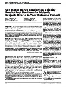
Fig. 1. Geometry used for calculating the field of a disk source. A circle of radius a represents the fiber cross section. The potential is obtained for the observation point P .

The potential function typical of active fibers, as described by Plonsey, necessarily arises from a double-layer source [15]. Legendre polynomial series expansions are used to compute the field of single- and double-layer disks. The differential contribution of a double-layer disk element to the potential at point is given by (1) where 4 ; intracellular and extracellular conductivities, respectively; spatial membrane potential; 1 1 3 5 2 1 2 4 6 2 1 ; Legendre polynomial of order 1. The value of the fiber depth is not smaller than 2.5 mm for an observation point located at the skin surface. Since a rather large value for the fiber radius is 25 m, the ratio 10 is of small magnitude. Also, and the functions , are on the same 1. Thus, consecutive terms of the order of magnitude for series expansion differ by approximately four orders of magnitude, justifying the use of the first term of the summation 0) as a good approximation for (1), which can then be ( expressed as and

(2)

1/ 2 4 and where This spatial description of the potential for any point, i.e., (abscissa ), leads to a temporal description of the potential at a given point located at the same radial distance from the fiber and at an axial distance from the stimulation or origination point. Assuming that the action potential (AP) wave propagates along the fiber with a constant velocity and noticing that is an odd function of , the time course of the potential at point can be obtained as (7) Since the AP travels at a constant velocity, the time function at a given position is a mirror image of at a given time . Taking this into account for the temporal and spaand changing from the spatial to the time tial derivatives of , a description of the potential at the domain by using observation point is obtained along the time variable

After substituting the expression for into the previous equation and rearranging it, the following result is obtained: (8) where 1/2

4

; ; factor that can be considered constant in nerve studies. It is in the order of 0.2 m m s [16]. Equation (8) can be expressed in a more compact form by means of a convolution operation over the time variable . This result is used to describe the surface single fiber action potential (SSFAP) and is given by

From Fig. 1 it can be observed that (9) (3) and (4) and making use of (3) and (4), (2) Knowing that can be written in Cartessian coordinates as follows: (5) The approximation made for representing the differential potential contribution holds well for computing the extracellular

is the time domain source and is where the convolution operator. In agreement with findings reported by Schoonhoven et al. [18], which were based on data reported in [14] and [17], this source can be considered independent of velocity for the estimation interval under consideration. Fig. 2. shows SSFAP waveforms representative of different velocities. They were generated using the model described above. The distance from the origination to the observation point used was 440 mm and the fiber depth was 8 mm. It can be noticed how the SSFAP duration decreases as velocity increases. On the other hand, the SSFAP amplitude increases as velocity gets higher. Fig. 3 shows that the order of this

142


Further grouping of the fiber contributions into velocity bins gives (11) where

Fig. 2. Set of SSFAP waveforms generated for different velocities according to the model presented. The fiber depth used was 8 mm and the distance from stimulation to recording was 440 mm.

number of bins; number of active fibers in bin ; average SSFAP of the active fibers belonging to velocity bin . Volume conductor theory was used in Section II to find the expression of the extracellular potential originated by an infinite single active fiber in an unbound isotropic medium for points located at distances corresponding to skin surface recording. The SSFAP was expressed by means of a time convolution operation involving the first derivative of the membrane potential, named [see (9)]. By substituting (9) into as the electrical source (11) the CNAP is given by (12) where

is the velocity chosen to represent bin . IV. CVD ESTIMATOR

The idea of using two CNAPs for the CVD estimation is very appealing, particularly when this implies that an estimate of the source is not necessary. The two-CNAP solution method proposed by Cummins [5] is appropriate when a convolution model of the CNAP such as that presented in (12) is obtained. Two CNAPs are recorded at two different distances and from the stimulation site. According to (12) they can be represented as (13)

and

(14) Fig. 3. The SSFAP amplitude change with velocity is illustrated. The order of the amplitude increase predicted by the volume conductor model is compared with a linear increase and a quadratic increase with velocity.

increment is higher than linearly proportional but smaller than a second-order increase with velocity.

, for 1 2 . where and both sides of Convolving both sides of (13) with leads to identical right-hand sides. Thus an esti(14) with mate of the s can be obtained by minimizing the error function given by the difference between the left-hand sides of the resulting equations. This error function can be written as

III. NERVE EVOKED RESPONSE The CNAP recorded at the skin surface can be expressed as the summation of the individual SSFAP (10)

(15) s is the The cost function chosen to minimize over the mean square error (MSE). Thus, the minimization problem can be stated as

where total number of active fibers; CV of fiber ; time variable.

(16) where

is the observation interval of interest.


The optimization problem is entirely defined by including the following equality and inequality constraints:

(17) (18) The constrained optimization problem presented by (16)–(18) can be solved using the Lagrange multiplier method. The objective function built using these equations satisfies the characteristics of a quadratic programming problem. Hence, a standard quadratic programming solution provided with software packages such as MATLAB v.5.3 was used to obtain the 1 . Due to (17), the estimates CVD estimate are given in relative number of active fibers as a percent of of the total number of active fibers. However, simulation results can be obtained in number of fibers if desired. V. SIMULATION The simulation of nerve data was based on the model described in Sections II and III. The elicited CNAPs were generated by first evaluating the volume conductor model of the SSFAP for each fiber CV and considering a common depth for all fibers underneath a given electrode. Then, all fiber contributions are summed as indicated in (10). The fiber velocities were originated following a Gaussian velocity distribution by means of a random number generator. employed The waveshape of the membrane potential was taken from [15] and time scaled according to data reported in [17]. The resulting SSFAP waveshapes showed a good agreement with graphical data reported in [18] despite the fact that the convolution models are different. The model proposed by Schoonhoven et al. is based on the second derivative of the membrane potential while the one presented in this paper is based on its first derivative. Two CNAPs need to be generated in order to test the CVD estimator, while an additional third channel is needed as well in order to test the prediction technique. This technique consists of predicting the CNAP waveform for a third channel not involved in the CVD estimation as explained below (see Section V-C). The simulated data correspond to CNAPs resembling somatosensory evoked potentials (SEPs) measured from the median nerve at the wrist, forearm, and elbow, while stimulating at the middle finger. The forearm channel is located approximately 60 mm away from the channel at the wrist. In the bipolar case, each channel consisted of a bipolar pair whose electrodes were spaced 20 mm along the nerve path. A. Evaluation of the Estimator Bias and Variance In order to assess the estimator performance in terms of its bias and variance, a rather large number of realizations is required. A velocity pdf, defined by a Gaussian distribution whose analytical function was known a priori, was used to generate 100 sets of propagation velocities each. is the number of active fibers and was chosen to be 900. Then, 100 CNAP pairs were generated based on the 100 velocity sets.

143

Monopolar recording configurations were assumed for the bias and variance evaluation. The two CNAPs involved in the CVD estimation were generated using distances from stimulation to recording sites of 175 mm for the wrist and 440 mm for the elbow channel. The nerve depths used 6 mm and 8 mm, respectively [8], [9]. were Fig. 4. shows the estimator performance averaged across data sets. The heights of the histogram bars represent the mean value of the 100 CVDs used to generate the 100 data sets. The 100 CNAP pairs were processed by the estimation algorithm and CVD estimates obtained. The mean values of the estimates are represented by the dots located at the middle of the vertical line segments, while the line segments extend to the standard deviation of the estimate error. This test was made under noise-free conditions. The estimator shows a very little bias since the difference between the mean value of the estimate and the mean value of the original distributions has a maximum value of 0.53 fibers for bin number 11. The standard deviations in the estimates are all less than 3.24 fibers, which was the figure found for bin number 14. The average standard deviation of the estimator errors computed across the 30 velocity bins was 1.02 fibers. B. Comparison of the Proposed Estimator and Cummins Implementation As mentioned in Section III, Cummins incorporated a revolutionary two-CNAP deconvolution technique to nerve CVD estimation. However, the estimator implemented did not account for the SSFAP waveshape dependence on velocity. The amplitude scaling factor chosen was inspired by data reported in the literature but lacking of physical/mathematical support. In order to obtain an idea of how different models will affect the estimation results, estimation was performed over two groups of 100 data sets each. The first group was generated assuming a uniform CVD extending over the interval 30–80 m/s, while the bimodal distribution used with the second group was called double Gaussian and is given by the following expression:

(19) Monopolar recording configurations were assumed, as well as a common nerve depth of 8 mm underneath each electrode. Stimulation to recording distances were 150 and 500 mm. Three different estimators processed each group of data: Cummins’, a second estimator that considers the SSFAP waveform entirely independent of velocity (neither amplitude nor duration scaling factors are present), and the volume conductor estimator proposed. The performances of the three estimators are shown in Fig. 5 for the first group of data sets. The mean values of the estimator errors obtained over 100 uniform distributions are plotted for 30 equally spaced velocity bins. It can be observed how Cummins’ estimator overestimates the low-velocity components and underestimates the high-velocity components. On the other hand, the reverse is true for the second estimator. Although this estimator is clearly biased as well, the magnitude of its bias is

144


Fig. 4. Performance of the nerve CVD estimator. The estimator mean (dots) and the standard deviation of the estimate error (vertical line segments) are represented for each bin.

Fig. 5. Estimator bias errors offered by Cummins’, the velocity-independent SFAP and the volume conductor implementations for a uniform distribution.

smaller than in Cummins’ case. The volume conductor estimator offers the best overall performance, although it is slightly degraded for the uppermost velocity bins. The performances of the three estimators are shown in Fig. 6 for the second group of data sets. The mean values of the estimator errors obtained over 100 double Gaussian distributions are plotted for 30 equally spaced velocity bins. The observations made previously for the uniform distribution hold well, except that in this case the volume conductor estimator performance is not deteriorated for the uppermost velocity bins. As can be appreciated from the results shown in Figs. 5 and 6, Cummins’ implementation overestimates the number of ac-

Fig. 6. Estimator bias errors offered by Cummins’, the velocity-independent SFAP and the volume conductor implementations for a double Gaussian distribution.

tive fibers having low CV, while it underestimates the high velocity ones. This behavior is expected given the quadratic amplitude-scaling factor Cummins assumed for the CNAP model and the order the simulated SSFAP amplitude increases with velocity, which is less than quadratic since the volume conductor model was used to generate the data. Also, the SSFAP duration predicted by the volume conductor model is shorter for high velocities and longer for low velocities. So, in order to compensate for this, Cummins’ estimator needs to allocate more fibers to the low velocities and less fibers to the high velocities.


Fig. 7. CVD estimates (left) and predicted CNAPs for channel 3 (right) are shown for

The CVD estimates obtained with estimators 1 and 2 were biased for the low- and high-velocity components. This is clearly due to the fact that a different model, the volume conductor model presented, was used for generating the CNAP data. Nonetheless, these results highlight the need for using an accurate CNAP model in order to obtain meaningful outcomes from a nerve CVD estimation technique. C. Estimator Performance Measure for Experimental Data As described earlier in Section IV, the deconvolution technique involves the use of two CNAPs, i.e., two recording channels. In order to evaluate the estimator performance through simulations, the original CVD used to generate the data fed to the estimator is available. Thus, a measure of the estimation error can be found and used as a performance index. This is not the case when processing experimental data. The need for assessing the estimator performance in the presence of data collected from a subject led to the addition of a third channel. can be used together with the tissue The CVD estimate in order to find the functions filter impulse responses and . Then, solving (13) and (14) for , through a and deconvolution operation, estimates of the source can be obtained from channels 1 and 2, respectively. Thus, estican be obtained from (13) and mates or predictions of (14) as follows: (20) where

1 2 and

The deconvolution operation when performed in the time domain is a stable operation for simulated data. However, when

145

SNR = 1[(A) and (B)] and SNR = 5 [(C) and (D)].

noise is considered, as present in the experimental signals, it can become unstable and a different approach is needed for its computation. A frequency domain approach that accounted just for the frequency range with significant CNAP information led to meaningful CNAP estimates. The estimates from (20) are compared to experimental or simulated signals corresponding to the independent third channel not involved in the CVD estimation. In order to assess the estimator performance, a percent MSE in the prediction of the thirrd channel is introduced as a performance index. It is given by

(21) This performance measure was used to evaluate the estimator immunity to noise as presented in the next section. D. Assessing the Estimator Performance in Presence of Noise Three CNAP signals were generated. They resembled bipolar recording configurations located at the wrist, forearm and elbow, while stimulating at the finger. The original or actual CVD used in the signal generation is shown in Fig. 7 (A) and (C). Fig. 7(A) also shows the CVD estimates obtained from the wrist and elbow signals in the absence of noise. The signal simulated for the forearm channel, as well as its prediction based on the CVD estimate, are shown in Fig. 7(B). The predicted CNAP (dashed curve) is the average CNAP estimate obtained from the wrist and elbow sources. Next, zero-mean Gaussian noise was added to the three channels. Since the amplifier gains and bandwidths used in the measurements were the same for all the channels, the noise levels are identical. To match these conditions the variance of the added noise was the same for each channel. The signal-to-noise (SNR)

146


TABLE I NOISE EVALUATION OF THE ESTIMATOR PERFORMANCE ON SIMULATED DATA. THE FOREARM PREDICTION MSE COMPUTED FOR THE SOURCES ESTIMATED AT THE WRIST (S ) AND ELBOW (S ) CHANNELS AND THE CVD ESTIMATE MAE, ARE SHOWN FOR FIVE DIFFERENT SNR CONDITIONS

ratio was computed as the ratio of the signal peak divided by the ), standard deviation of the noise. The SNR of channel 2 ( the elbow channel, was taken as the reference for assessing the estimator immunity to noise. The signal corresponding to this channel had the lowest level, which means the lowest SNR as well. The noise power was progressively increased such that the was gradually reduced from 50 down to five, as shown in the Table I. The CVD estimates and the predictions of the forearm channel corresponding to the poorest SNR case are presented in Fig. 7(C) and (D), respectively. Two performance measures are presented in Table I. The second column offers the values of the mean absolute error (MAE) in the velocity estimate. The MAE is expressed in percent of the total number of fibers and is given by

Fig. 8. CVD estimate obtained having overestimated the distances from stimulation to recording sites at the wrist by 20 mm and at the elbow by 40 mm.

(22) The last two columns offer the percent MSE in the prediction of the forearm channel (see Section V-C). The two prediction errors shown correspond to the waveforms predicted using the source estimated at the wrist ( ) and the source estimated at the elbow ( ). Due to the random characteristics of the Gaussian noise added to the simulated signals the performance indexes shown in Table I were found after averaging over ten runs. This was done in order to reduce the variability of the results over distinct random noise realizations so the numbers obtained were representative. It can be observed from Table I that as the SNR gets poorer the as low as 5 the CVD esMSE measures get larger. For an timate generally presents an error greater than 0.5%. This represents an error greater than 10% when expressed as a percentage of the average number of fibers per bin in a 20-bin histogram. However, the general shape of the CVD is still estimated reasonably well as can be observed in Fig. 7(C). E. Effects of the Errors Introduced in the Estimation of Distances and Depths Parameters obtained through estimation or measurements are prone to errors. Even when the position and course of nerves have been studied through magnetic resonance imaging techniques and described in anatomy books, there is always variability from subject to subject and even from day to day for the same subject. Moreover, nerve fibers do not follow straight-line

Fig. 9. CVD estimate obtained having underestimated the distances from stimulation to recording sites at the wrist by 20 mm and at the elbow by 40 mm.

paths. Curved nerve paths have also been considered for computing the potential due to an active fiber [26]. Since errors in the distance and depth parameters are likely to occur, the ability of the estimator to cope with them was tested. First, the distances from the stimulation site to the recording sites were altered in the estimator. The result presented in Fig. 8 correspond to an error of 20 mm for the finger-wrist distance and an error of 40 mm for the finger-elbow distance, which conveys an error of 20 mm in the distance between the wrist and elbow recording channels. As signalled by the block arrows, the CVD estimates obtained are shifted to the right with respect to the original bimodal CVD used in the simulation of the CNAP signals involved in the estimation. A bimodal distribution was used in this study in order to observe errors not only involving the middle section of estimation interval but the lower and upper sections of it as well. Fig. 9 shows the equivalent results when the distances are underestimated. In this case, the estimates are shifted toward


the low velocities. The shifts occur in the expected direction in all cases since the estimator attempts to compensate for an excess or lack of distance by increasing or decreasing velocity, respectively. The estimator is not extremely sensitive to errors in the distance parameters if one considers that 40 mm would be a rather large error. Despite the shift the general shape of the CVD is preserved in the estimation for errors in the interchannel distance of 20 mm. The sensitivity of the nerve CVD estimator to errors in the estimation of nerve depths was tested by upsetting this parameter in the estimator implementation. The depth values used in the generation of the CNAP signals, referred as the actual depths, were 8 mm for both electrodes forming the bipolar pair located at the wrist and 10 mm for the electrode pair located at the elbow. When introducing errors of 50% of the true values (4 and 5 mm, respectively) in the same direction, i.e., overestimating or underestimating the depths for both channels, the CVD estimates were not affected significantly. Although, it was apparent that underestimation is more critical [9]. Next, errors going in opposite directions were combined, which means that depths were overestimated for one channel and underestimated for the other channel. When introducing a 25% percent error in the depth estimation (2 and 2.5 mm, respectively), the CVD estimates obtained still keep the CVD estimation error low and the shape of the original distribution is preserved. In this case, underestimation of the nerve depth at the wrist combined with overestimation of the depths at the elbow affect the estimator performance slightly more. A more significant deterioration on the CVD estimate was observed when these errors are 50% of the actual depth values and acting in opposite directions [9]. However, a 4–5 mm depth is unlikely so it is not among the depth values regularly used in the CVD estimation. Consequently, a 50% underestimation of the depths is an extreme case and the estimator is not expected to be affected this much in practice. VI. EXPERIMENTAL RESULTS This research involving human subjects was approved by the university research ethics committee. All guidelines as set down by the Canadian Tri-Council policy on research involving human subjects were followed including the subjects’ informed consent. The median nerve was stimulated using electrodes located at the middle finger and spaced from 20 to 30 mm. The nerve-evoked response was recorded using surface circular electrodes of 6 mm radius. There were three recording sites located along the path of the median nerve. The most distal was located close to the wrist. The signal recorded at this site was named CNAP1 (channel 1). The second site was placed on the elbow and the signal recorded at this site was named CNAP2 (channel 2). A third channel was located at the forearm approximately 60 mm proximal to the first and the signal recorded at this site was named CNAP3 (channel 3). Each channel consisted of a bipolar pair with an interelectrode spacing of 20 mm. The nerve-evoked responses were averaged by a Brüel and Kjær signal analyzer. A total of 2000 responses were averaged in

147

TABLE II VALUES OF THE PREDICTION MSE OF THE FOREARM CHANNEL (CHANNEL 3) BASED ON CVD ESTIMATES OBTAINED USING THE WRIST CHANNEL (CHANNEL 1) AND THE ELBOW CHANNEL (CHANNEL 2)

order to obtain the enhanced time signals for each data set. The subject was prone on a bed and stimulation was applied using a constant voltage Grass stimulator at a rate of one pulse every 391.7 ms until 2000 data frames were collected and averaged for all three channels. The stimulus duration used was 0.1ms and its intensity varied according to the subject’s perception threshold. The bandwidth of the analogue filter amplifier was set from 10 Hz–10 kHz. The gains of the pre-amp and amplifier stages were typically set to 100 and 500, respectively. The analog-to-digital (A/D) sampling frequency was 65.574 kHz per channel. Since all channels exhibited SNRs below 200 the 15-bit A/D converter quantization noise is well below the additive system noise floor remaining after the signal averaging. The discrete-time signals were passed through a low-pass filter with cut-off frequency of 3 kHz in order to further improve the SNR. Then, the dc component was removed as well. A. Assessment of the Estimation Results CVD estimates were based on channels 1 and 2 since this pair offers the best delay resolution and lowest sensitivity to parameter errors due to the spacing between the channels involved [9]. According to the prediction of the forearm channel, the CVD estimates obtained from data sets NN, OO, TT, and UU are good (see Table II). The prediction MSE is smaller than 16% for these data sets. The CVD estimate obtained for data set WW has the highest prediction MSE, 38%, among the estimates based on the (wrist, elbow) pair. Thus, the CVD estimate corresponding to data set WW may not be as good or reliable as the rest. A typical CVD estimate and the forearm prediction are shown in Figs. 10 and 11, respectively, for subject , data set OO. Fig. 11 shows that the prediction closely match the recorded waveform at the forearm. The percent MSE in the prediction, used as a figure of merit for the CVD estimator performance, presents a 10.4% and a 15.1%, respectively, for each of the sources as shown in Table II. These facts suggest that the CVD estimate obtained is reasonably good. B. Comparison With Cummins’ Estimator According to simulation results Cummins’ estimator behaves differently than the volume conductor estimator. Fig. 12(A) and (C) present the CVD estimates obtained by both estimators from a (wrist, elbow) CNAP pair collected from subject . The reconstructed, or predicted, CNAPs for the forearm channel are also plotted together with the actual signals in Fig. 12(B) and (D).

148


by the simulation results). Also, the signals predicted for the forearm channel by the volume conductor estimator are closer to the recorded ones than those predicted with Cummins’ estimator [see Fig. 12(B) and (D)]. The prediction MSEs obtained with the volume conductor estimator are smaller by at least a factor of two than those obtained with Cummins’. This is consistent across all experimental data sets collected when using the (wrist, elbow) pair in the CVD estimation, as can be noticed from Table III, with the exception of data set WW for which the volume conductor prediction MSEs are smaller by factors of 1.3 and 1.4. C. Repeatability Study

Fig. 10. Volume conductor CVD estimate obtained from the wrist and elbow CNAPs recorded from subject P , data set OO.

Fig. 11. Prediction of the forearm channel based on the CVD estimate shown in Fig. 10 obtained with the volume conductor estimator from subject P , data set OO.

Table III gathers the prediction MSE indexes for all six data sets presented in the previous section. The prediction of the channel not involved in the CVD estimation makes use of a weighted sum of the tissue filter impulse responses corresponding to the velocity bins involved in the estimation. The weighting factors are the values of the CVD estimate itself. In the case of the volume conductor estimator, the impulse responses are provided by the model described in Section II. Cummins’ implementation uses impulses (Dirac delta functions) shifted by the corresponding delays and weighted by a quadratic amplitude-scaling factor instead. These were called “shaping functions” [5]. The same “shaping functions” used in Cummins CVD estimation are employed here as impulse responses in the prediction of the channel not involved in the CVD estimation. As can be observed from Fig. 12(A) and (C), the CVD estimate offered by Cummins’ method favors the low-velocity components more than the volume conductor estimates (as predicted

In order to study the repeatability of the results obtained with the volume conductor estimator proposed in this work, 12 data sets were collected from subject A. Three data sets were from Monday (day 1), five from Tuesday (day 2), and four from Thursday (day 3) of the same week. As far as possible, all experimental parameters, including the location of the stimulating and recording electrodes, stimulation intensity, frequency and pulse duration, were the same over all of the sets. The average CVD estimates shown in Fig. 13 were obtained based on data sets collected on different days from subject A. It can be observed that the shape of the estimated CVD exhibits minor differences from day to day. The lowest mean CV (44.0 m/s) corresponds to day 2, the intermediate mean CV (45.1 m/s) is from day 3, and the highest mean CV (46.1 m/s) belongs to day 1. These results are in agreement with the latency variation of the SEPs. The CNAPs recorded at the three sites (wrist, forearm, and elbow) exhibit a noticeable time shift from day to day. These shifts are in the direction suggested by the CVD estimates, that is, the more low-velocity components are present in the CVD estimates of Fig. 13 the later the CNAPs occurred. The CVD estimates shown in Fig. 14 were obtained from the data sets collected on the second day. These plots show very little discrepancy among the results obtained on the same day. Overall, the results are consistent and the uncertainty introduced by the CNAP latency variations across data sets is in the order of 2 m s and does not significantly affect the shape of the CVD estimate. D. SNR Assessment The experimental data collected from subject A during four different days were used to assess the effect of noise on the estimator performance. The SNR was estimated for each of the data sets, as well as the average SNR for each day. They are presented in Table IV together with the percent MSE in the prediction of the forearm channel. The SNR, previously defined in Section V-D, was found as the ratio of the peak value of the CNAP signal divided by the estimate of the noise standard deviation. The noise standard deviation estimate was made over the segments of data not containing CNAP signal. For instance, the standard deviation for channel 2 was computed from the segment of data comprised by the interval [15 ms, 30 ms] after the stimulus onset. ranged from 7 to 15 V/V and higher in The estimated some cases. Despite the statistical variability that may be present


149

Fig. 12. CVD estimates and predictions of the forearm channels obtained with Cummins’ estimator [(A) and (B)] and the volume conductor estimator proposed [(C) and (D)]. The wrist and elbow CNAPs recorded from subject J , data set TT, were used by the two-CNAP estimation techniques. TABLE III VALUES OF THE PREDICTION MSE OF THE FOREARM CHANNEL OBTAINED WITH CUMMINS ESTIMATOR (CUMM. ESTIM.) THE CORRESPONDING VALUES OBTAINED WITH THE VOLUME CONDUCTOR ESTIMATOR (V.C. ESTIM.) ARE INCLUDED FOR COMPARISON

due to averaging just three or four data sets per day, the mean prediction error for day 3 is the smallest, which is in agreement . However, when with day 3 presenting the largest mean comparing the error range resulting from the prediction of experimental data with those associated with the prediction of sim, the prediction error is larger ulated data, for the same in the case of the experimental data. This margin is associated with errors in the experimental CVD estimate caused in part by mismatch on the distance and depth parameters, which also contribute directly to a larger error in the prediction of the forearm channel. For instance, the CVD estimate obtained for day 2 is indeed slightly biased toward the low velocities with respect to estimates from other days. This may be an erroneous result if the large delays present in the wrist and elbow channels were not accounted for by introducing the appropriate distance corrections in the estimator.

Fig. 13. Mean CVD estimates obtained from subject A on different days. They show the consistency achieved by the CVD estimator across different days.

The SNR at each of the two recording site affects the source estimates differently, particularly when considering that the deconvolution operation used to estimate the source was implemented in the frequency domain by means of a division. Thus, it is expected that the predictions based on the wrist CNAP (Pre) are more accurate than those based on the diction ) as shown in Table IV. elbow CNAP (Prediction VII. CONCLUSION The estimator presented in this paper is seen to be robust for the levels of noise present in the experimental signals. For

150


Fig. 14. CVD estimates obtained from five different data sets collected from subject A on day 2. They show the consistency achieved by the CVD estimator on a particular day.

TABLE IV ESTIMATOR PERFORMANCE ON EXPERIMENTAL DATA. THE FOREARM PREDICTION MSE COMPUTED FOR THE SOURCES ESTIMATED AT THE WRIST (S ) AND ELBOW (S ) CHANNELS AND THE SNR CONDITIONS ARE SHOWN FOR 15 DATA SETS COLLECTED FROM SUBJECT A DURING THREE DAYS

instance, for a typical experimental of ten in the elbow channel the MSE obtained in the prediction of the forearm channel was in the order of 5% for simulations and 10%–15% for experimental data. This difference between simulations and experimental results is expected since experimental conditions are affected by parameter errors that were not included in the SNR study done through simulations. The estimator may be affected to a greater extent if errors of 50 of the actual depth values are introduced. However, this range of depth errors is considered rather extreme so the estimator performance should not be considerably deteriorated in practice due to errors in the depth parameters. Errors in the

distance parameters in the order of 20–40 mm may cause a shift in the CVD estimate, however, the shape of the actual CVD should not be significantly affected in the resulting estimate. The experimental results showed that the channel pair with the largest spacing and stimulation-recording distances, the (wrist, elbow) pair, offers the most accurate prediction of a third channel not involved in the CVD estimation. The lowest prediction MSE corresponds to the forearm channel over the prediction MSE obtained for the wrist or elbow channels and is used as a figure of merit to claim that this channel pair (wrist, elbow) offers the best CVD estimation results. This approach to validation of the experimental results was extended


to Cummins’ estimator. The comparison of both simulation and experimental results, using the prediction of channel 3 as an impartial index, clearly shows an improved performance from the volume conductor estimator proposed in this work whose prediction MSE index was half that of Cummins. Considering that the shift observed in the CVD estimates across different days is consistent with latency changes on the nerve responses and that there is no significant change in the shape of the estimated CVDs, the estimator results manifest to be successfully repeatable. Nonetheless, it is desired to minimize the variability in the latency shifts of the signals from one day to the next and within the same day, such that the results obtained with the use of this technique are not affected by this perturbing factor. REFERENCES [1] A. T. Barker, B. H. Brown, and I. L. Freeston, “Determination of the distribution of conduction velocities in human nerve trunks,” IEEE Trans. Biomed. Eng., vol. BME-26, pp. 76–81, Feb. 1979. [2] F. Buchthal and A. Rosenfalck, “Evoked action potentials and conduction velocity in human sensory nerves,” Brain Res., vol. 3, pp. 1–122, 1966. [3] A. I. Cruz-Martínez, M. Barrio, and M. Guillén, “Aspectos electrofisiolólogicos de la neuropatía urémica. I: Electromiografía, conducción nerviosa motora y sensitiva y respuestas reflejas,” Rev. Clin. Esp., vol. 156, pp. 419–424, 1980. [4] K. L. Cummins, D. H. Perkel, and L. J. Dorfman, “Nerve fiber conduction-velocity distributions. I. Estimation based on the single-fiber and compound action potentials,” Electroenceph. Clin. Neurophysiol., vol. 46, pp. 634–646, 1979. [5] K. L. Cummins, L. J. Dorfman, and D. H. Perkel, “Nerve fiber conduction-velocity distributions. II. Estimation based on two compound action potentials,” Electroenceph. Clin. Neurophysiol., vol. 46, pp. 647–658, 1979. [6] K. L. Cummins and L. J. Dorfman, “Nerve fiber conduction velocity distributions: Studies of normal and diabetic human nerves,” Ann. Neurol., vol. 9, pp. 67–74, 1981. [7] L. J. Dorfman, K. L. Cummins, G. M. Reaven, J. Ceransky, M. S. Greenfield, and L. Doberne, “Studies of diabetic polyneuropathy using conduction velocity distribution (DCV) analysis,” Neurology, vol. 33, pp. 773–779, 1983. [8] J. A. González-Cueto and P. A. Parker, “Deconvolution estimation of nerve and muscle conduction velocity distribution,” in Proc. Chicago 2000 World Congr. Medical Physics and Biomedical Engineering, July 2000. [9] J. A. González-Cueto, “An Investigation of Non-Invasive Techniques for the Estimation of Conduction Velocity Distributions in Skeletal Muscles and Nerve Bundles,” Ph.D. dissertation, Dept. Elect. Comput. Eng., Univ. New Brunswick, Fredericton, Canada, 2001. [10] D. Gu, R. E. Gander, and E. C. Crichlow, “Determination of nerve conduction velocity distribution from sampled compound action potential signals,” IEEE Trans. Biomed. Eng., vol. 43, pp. 829–838, Aug. 1996. [11] Y. Harati, “Diabetic peripheral neuropathies,” Ann. Intern. Med., vol. 107, pp. 546–559, 1987. [12] G. Hirose, Y. Tsuchitani, and J. Huang, “A new method for estimation of nerve conduction velocity distribution in the frequency domain,” Electroenceph. Clin. Neurophysiol., vol. 63, pp. 192–202, 1986. [13] Z. L. Kovacs, T. L. Johnson, and D. S. Sax, “Estimation of the distribution of conduction velocities in peripheral nerves,” Comput. Biol. Med., vol. 9, no. 4, pp. 281–293, 1979. [14] A. S. Paintal, “Effects of temperature on conduction on single vagal and saphenous myelinated nerve fibers of the cat,” J.Physiol., vol. 180, pp. 20–20, 1965. [15] R. Plonsey, “The active fiber in a volume conductor,” IEEE Trans. Biomed. Eng., vol. BME-21, pp. 371–381, 1974.

151

[16] R. Schoonhoven and D. F. Stegeman, “Models and analysis of compound nerve action potentials,” Crit. Rev. Biomed Eng., vol. 19, pp. 47–111, 1991. [17] R. Schoonhoven, D. F. Stegeman, and J. P. C. De Weerd, “The forward problem in electroneurography—I: A generalized volume conductor model,” IEEE Trans. Biomed. Eng., vol. BME-33, pp. 327–334, Mar. 1986. [18] R. Schoonhoven, D. F. Stegeman, and V. A. Oosterom, “The forward problem in electroneurography—II: Comparison of models,” IEEE Trans. Biomed. Eng., vol. BME-33, pp. 335–341, Mar. 1986. [19] R. Schoonhoven, D. F. Stegeman, V. A. Oosterom, and G. F. M. Dautzenberg, “The inverse problem in electroneurography—I: Conceptual basis and mathematical formulation,” IEEE Trans. Biomed. Eng., vol. 35, pp. 769–777, Oct. 1988. [20] K. W. Seneviratne and O. A. Deiris, “Peripheral nerve function in chronic liver disease,” J. Neurol. Neurosurg. Psychiat., vol. 33, pp. 609–609, 1970. [21] D. F. Stegeman, R. Schoonhoven, G. F. M. Dautzenberg, and J. Moleman, “The inverse problem in electroneurography—II: Computational aspects and evaluation using simulated data,” IEEE Trans. Biomed. Eng., vol. 35, pp. 778–788, Oct. 1988. [22] Y. X. Tu, A. Wernsdörfer, S. Honda, and Y. Tomita, “Estimation of conduction velocity distribution by regularized-least-squares method,” IEEE Trans. Biomed. Eng., vol. 44, pp. 1102–1106, Nov. 1997. [23] M. D. Wells and S. N. Gozani, “A method to improve the estimation of conduction velocity distributions over a short segment of nerve,” IEEE Trans. Biomed. Eng., vol. 46, pp. 1107–1120, Sept. 1999. [24] A. Wichman, F. Buchthal, C. H. Pezeshkpour, and A. S. Fauci, “Peripheral neuropathy in hypereosinophilic syndrome,” Neurology, vol. 35, pp. 1140–1145, 1985. [25] A. Wichman, F. Buchthal, C. H. Pezeshkpour, and R. E. Greg, “Peripheral neuropathy in abetalipoproteinemie,” Neurology, vol. 35, pp. 1279–1281, 1985. [26] S. Xiao, K. C. McGill, and V. R. Hentz, “Action potentials of curved nerves in finite limbs,” IEEE Trans. Biomed. Eng., vol. 42, pp. 599–607, June 1995.

José A. González-Cueto received the B.Eng. degree in automatic control from the Central University of Las Villas (UCLV), Santa Clara, VC, Cuba, in 1991, the M.Sc.E. degree in telecommunications from UCLV in 1996, and the Ph.D. degree in electrical and computer engineering from the University of New Brunswick (UNB), Fredericton, NB, Canada, in 2001. He is currently with the NeuroMuscular Research Center at Boston University, Boston, MA, as a Research Associate. His research interests include processing techniques applied to neuromuscular signals, DSP algorithms, and real-time implementations. Dr. González-Cueto is a student member of the Canadian Medical & Biological Engineering Society (CMBES) since 1997.

Philip A. Parker (S’70–M’73–SM’86) received the B.Sc. degree in electrical engineering from the University of New Brunswick (UNB), Fredericton, NB., Canada, in 1964, the M.Sc. degree from the University of St. Andrews, St. Andrews, Scotland, in 1966, and the Ph.D. degree from UNB in 1975. In 1966, he joined the National Research Council of Canada as a Communication Officer and the following year he joined the Bioengineering Institute, UNB, as a Research Associate. In 1976, he was appointed to the Department of Electrical Engineering, UNB and currently holds the position of Professor in that department. He is also a Research Consultant to the Bioengineering Institute, UNB. His research interests lie mainly in the area of biological signal processing.