Keywords: Segmentation · Multiple Sclerosis · Convolutional Neural. Network · ... image-processing operations, and machine learning approaches. ... (whole-brain) fully convolutional end-to-end encoder-decoder network proposed.
Deep 2D Encoder-Decoder Convolutional Neural Network For Multiple Sclerosis Lesion Segmentation in Brain MRI Shahab Aslani1,2 , Michael Dayan1 , Vittorio Murino1,3 , and Diego Sona1,4 1
Pattern Analysis and Computer Vision (PAVIS), Istituto Italiano di Tecnologia (IIT), Genoa, Italy 2 Science and Technology for Electronic and Telecommunication Engineering, University of Genoa, Italy 3 Dipartimento di Informatica, University of Verona, Italy 4 NeuroInformatics Laboratory, Fondazione Bruno Kessler, Trento, Italy {name.surname}@iit.it
Abstract. In this paper, we propose an automated segmentation approach based on a deep two-dimensional fully convolutional neural network to segment brain multiple sclerosis lesions from multimodal magnetic resonance images. The proposed model is made as a combination of two deep subnetworks. An encoding network extracts different feature maps at various resolutions. A decoding part upconvolves the feature maps combining them through shortcut connections during an upsampling procedure. To the best of our knowledge, the proposed model is the first slice-based fully convolutional neural network for the purpose of multiple sclerosis lesion segmentation. We evaluated our network on a freely available dataset from ISBI MS challenge with encouraging results from a clinical perspective. Keywords: Segmentation · Multiple Sclerosis · Convolutional Neural Network ·
1
Introduction
Multiple Sclerosis (MS) is one of the most common demyelination diseases having direct effects on the central nervous system, especially on white matter (WM), which can be visualized through magnetic resonance imaging (MRI) scans. The detection of all MS lesions is an important task as it can help characterizing the progression of the disease and monitoring the efficacy of a candidate treatment [14]. In literature, there are both manual and automatic methods for MS lesion segmentation. Manual segmentation usually provides accurate results with the drawbacks of being time-consuming, affected by expert skills and biased towards a given expert. This highlights the importance of automatic segmentation methods, which can be faster, not affected by the expertise variability and unbiased [4].
2
S. Aslani et al.
Methods of automated MS lesion segmentation can be arbitrarily classified in two main types: empirical approaches typically based on a heuristic series of image-processing operations, and machine learning approaches. Image-processing based methods are faster but generally depend on the manual set-up of specific parameters, for example, the choice of thresholds, as in He et al. [7], where an adaptive procedure segments unhealthy regions with a multi-step pipeline of morphological operations. On the contrary, machine learning based approaches particularly supervised methods can be slower but learn automatically from a training dataset previously labeled by an expert. For example, Jesson et al. [8] proposed a three-stage pipeline to discriminate healthy tissues from lesions, where intensity distributions were used to train a random forest classifier. Recently, deep learning methods, in particular, convolutional neural networks (CNNs), have shown excellent performance with various applications [9]. One of the most important advantages of these methods over other supervised algorithms is that they can learn themselves how to design features directly from data during the training procedure. It is important to mention that over the last years, CNNs have also been used in biomedical image analysis with state-of-theart results in different problems [13]. Regarding the literature, there exist a few proposed methods based on CNNs for segmenting MS lesions. In [1], a three-dimensional (3D) CNN is designed to use shortcut connections between layers of the network, which allow concatenating the features from deep layers to shallow layers. Recently, Valverde et al. [15] proposed a patch-based method relying on a cascade of two 3D CNNs. In this approach, the extracted volumetric patches are used to train the first network. Then, a second network is used to refine the training on samples misclassified by the first network. In this paper, we present a pipeline for automatic MS lesion segmentation based on two-dimensional (2D) CNNs. In this work, we concentrated on whole-brain segmentation in order to avoid some common problems like the neglect of global information of patch-based approaches, and the overfitting of 3D segmentation due to the small sample set issue. The CNN architecture used in this approach is a modified version of Residual Network (ResNet) [6] which has been proposed for image classification. To the best of our knowledge, this is the first slice-based (whole-brain) fully convolutional end-to-end encoder-decoder network proposed for MS lesion segmentation. The robustness of the method is improved by exploiting the volumetric slicing in all three possible imaging planes (axial, coronal and sagittal). Indeed, we used different imaging axes of each 3D input MRI in an ensemble framework to exploit the contextual information in all three anatomical planes. Moreover, this model can be used as a multi-modal network to make use of all of the information available within each within each MRI modality available, typically fluid-attenuated inversion-recovery (FLAIR), T1-weighted (T1w), and T2-weighted (T2w).
Title Suppressed Due to Excessive Length
3
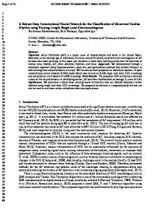
Fig. 1. Feature extraction pipeline. From each original 3D MRI image, axial, coronal and sagittal planes were extracted for each modality. Last column: in our specific application which 3 modalities were used (FLAIR, T1w, T2w), multi-channel slices (represented here as RGB images) were created by grouping together the corresponding slices of each modality.
2 2.1
Method Input Data Preparation
From each original volumetric MRI modality, axial, coronal and sagittal planes are considered by extracting 2D slices along the x, y, z axes of the 3D image. Since the size of the imaging planes differed according to the imaging axes, we zero padded each slice (while centering the brain), so that to obtain the same consistent size irrespective of the imaging plane. Further, the same consistent size was applied across modalities. Then, slices belonging to each plane orientation and each modality were stacked together to create a single multi-channel input stack. Since three modalities were used in our experiments, the obtained multichannel slices included three channels which can be represented as RGB images. Figure 1 illustrates the described procedure using three modalities, FLAIR, T1w, and T2w. 2.2
Network Architecture
Recently very deep CNNs showed outstanding performance in computer vision problems. In particular, ResNet [6] based on residual connections, gave significant improvement in image recognition tasks. Deep networks are hard to train because of the vanishing gradient problem during the back-propagation procedure. Therefore, when the network goes deeper, its performance gets saturated. The authors in [6] addressed the mentioned problem by proposing the network
4
S. Aslani et al.
called ResNet. The main idea of the ResNet is to use identity shortcut connection between layers of the network which have some benefits like preventing of vanishing gradient and also not adding computational complexity to the network. In this work, we modified ResNet50 (version with 50 layers) for a pixel-wise segmentation task inspired by the idea of Fully Convolutional Networks (FCNs) [10]. The easiest way to convert a ResNet to a segmentation network is to replace the last prediction layer with a dense pixel-wise prediction layer as described in FCNs. Since the output of the last convolutional layer of ResNet is very coarse compared with the input image resolution (32 times smaller than the original image) upsampling such high level feature maps with a simple operation like bilinear interpolation as described in FCNs is not an effective solution. Therefore, in order to address this problem, we propose a multi-pass upsampling network using the advantages of multi-level feature maps with skip connections. In deep networks, features from deep layers include high-level semantic information. On the contrary, features from early layers contain low-level spatial information. It was shown that features from middle layers also provide information which can be effective to increase the performance of the segmentation [13]. Therefore, combining multi-level features from different stages of the network makes the feature map richer than just using single scale feature maps. The intuition behind this work is to use these multi-level feature maps by adding multiple upsampling network with skip connections [13] to the ResNet output of all intermediate layers. The diagram of the proposed network for segmentation can be seen in Figure 2. We divided the ResNet50 into 5 blocks in the downsampling part according to the resolution of feature maps. In the upsampling subnetwork, the encoded features from different scales are decoded step by step using upsampling fused features (UFF) blocks. Each UFF block includes one upconvolutional layer with kernel size 2 × 2 and stride 2, one concatenation or fusion layer and two convolution layers with kernel sizes 3 × 3. After each layer, a rectifier linear activation function (ReLU) is applied [12]. The upconvolutional layer is used to transform low-resolution feature maps into the higher resolution maps. Then a simple concatenation layer is used for combining the two sets of input feature maps. Two convolution layers are further used for adaptation as described in [13], and the output goes to the next block. The number of feature maps after each UFF block is halved. At the end of the network, a soft-max layer of size 2 is used to get output probability maps, identifying pixel-wise positive (lesion) or negative (non-lesion) classes.
3 3.1
Experiments Data
To evaluate the proposed model, we used the dataset from ISBI 2015 Longitudinal MS Lesion Segmentation Challenge; which includes 19 subjects divided into two sets, 5 subjects for training and 14 subjects for testing. All training and testing data have the same 1mm-isotropic resolution. Each subject has MRI
Title Suppressed Due to Excessive Length
5
Fig. 2. a) General framework of the proposed network for MS segmentation. The first sub-network (ResNet50) encodes the input 2D slices into different resolutions. This sub-network was divided into 5 blocks with respect to the resolution of the representations during the encoding. The second sub-network (Upsampling) decodes the representations provided by the encoder network. This sub-network gradually converts low-resolution representations back to the original resolution of the input image using UFF blocks. b) Details of the proposed UFF block. Each UFF block has two set of input representations with different resolutions. This block is responsible to upsampling the low-resolution representations and combines them with high-resolution representations.
data with a different number of time-points, normally ranging between 4 to 6. Moreover, for each time-point, T1w, T2w, proton density-weighted (PDw), and FLAIR image modalities were provided. All training images have been segmented manually by two different raters and the segmented images are publicly available. For the test set, there is no public available ground truth. In order to evaluate the performance of the proposed method over the test dataset, the associated lesion binary mask must be submitted to the challenge website for evaluation [2].
6
3.2
S. Aslani et al.
Training and Testing
To train the proposed CNN, firstly, a training dataset was created using the pipeline mentioned in the previous section. In order to remove uninformative samples from the whole training set, a subset was determined by selecting only slices with at least one lesion pixel. This meant that 2D slices without lesions were omitted from the training set. In order to optimize network weights and early stopping criteria, we split the training dataset into different training and validation sets depending on the experiments as described in the following section. According to the network initialization, in the first subnetwork, the pretrained ResNet50 on ImageNet was used and the weights from the second subnetwork (Upsampling) were randomly initialized. Adaptive learning rate method (ADADELTA) [16] was used to tune the learning rate and a binary cross-entropy was used as loss function. The maximum number of training epochs was fixed to 500, and the best model was selected according to the validation set. We evaluated then the proposed network with unseen test data with respect to the corresponding experiments. For each subject, we first extracted all the slices from the test set, following the approach described in the previous section. Feeding each 2D slice to the network, we got as output the associated 2D binary lesion classification map. Since the original data was duplicated three times in the input, once for each slice orientation (coronal, axial, sagittal), concatenating the binary lesion maps belonging to the same orientation resulted in three 3D lesion classification maps. These three lesion maps were combined via majority voting (the most frequent lesion classification was selected). We implemented our proposed model in Keras [3] using a Nvidia GTX Titan X GPU. 3.3
Data Augmentation
As suggested in [5], simple off-line data augmentation was applied to the training dataset in order to increase training samples. Increasing training samples has been shown to increase the performance of the network. Therefore, we increased the number of the samples by a factor of 5 simply by either rotating each extracted slice by 4 possible angles (5◦ , 10◦ , -5◦ , -10◦ ) and flipping (right to left) of the images with their original rotation (no combination of flipping and rotation were included in the data augmentation procedure). 3.4
Evaluation
For evaluation purposes, two different experiments were implemented according to the availability of ground truth. In the first experiment, we ignored the official ISBI test set so that to only consider data with the available ground truth. In order to get a fair result, we did a leave-one-out cross-validation training (at subject level: 3 subjects for training, 1 subject for validation and 1 subject for testing). In this experiment, Dice Similarity Coefficient (DSC), Lesion-wise True Positive Rate (LT P R), and Lesion-wise False Positive Rate (LF P R) measures
Title Suppressed Due to Excessive Length
7
Fig. 3. An example of our network results in the axial, coronal and sagittal planes. First column: original FLAIR modality from different views, second column: ground truth related to the rater 1, third column: ground truth related to the rater 2, last column: segmentation output from the proposed method.
were used for evaluation. The DSC is computed as; DSC = (2 × T P )/(F N + F P + 2 × T P )
(1)
Where T P , F N and F P indicate the true positive, false negative and false positive voxels respectively. LT P R denotes the number of lesions in the reference segmentation that overlap with a lesion in the output segmentation, divided by the number of lesions in the reference segmentation (lesion recall). LF P R denotes the number of lesions in the output segmentation that do not overlap with a lesion in the reference segmentation, over the total number of lesions in the produced segmentation (lesion precision). For the second experiment, the official ISBI test set was used as our test set so the ground truth was not available. We trained the network using leaveone-out cross-validation over all 5 subjects in the training set (4 subjects for training and 1 subject for validation). We evaluated the ensemble of 5 trained models on the test set and then for a final prediction, we did majority voting over all classifiers. The 3D output binary lesion maps were submitted to the website of ISBI for evaluation purposes. In this experiment, a score is measured
8
S. Aslani et al.
Table 1. Comparison of our method with the other state-of-the-art methods. GT1 and GT2 show that the corresponding model was trained using annotation provided by rater 1 and rater 2 as the ground truth respectively. Method Rater 1 Rater 2 Jesson et al. [8] Maier et al. [11] Maier et al. [11] Brosch et al. [1] Brosch et al. [1] Ours (GT1) Ours (GT2)
(GT1) (GT2) (GT1) (GT2)
DSC 0.7320 0.7040 0.7000 0.7000 0.6844 0.6833 0.6980 0.6940
Rater 1 LTPR 0.8260 0.6111 0.5333 0.5555 0.7455 0.7833 0.7460 0.7840
LFPR 0.3550 0.1355 0.4888 0.4888 0.5455 0.6455 0.4820 0.4970
DSC 0.7320 0.6810 0.6555 0.6555 0.6444 0.6588 0.6510 0.6640
Rater 2 LTPR 0.6450 0.5010 0.3777 0.3888 0.6333 0.6933 0.6410 0.6950
LFPR 0.1740 0.1270 0.4444 0.4333 0.5288 0.6199 0.4506 0.4420
online (using the challenge website) according to the results on that test set. As described in [2], the mentioned score is a weighted average of different metrics including DSC, LT P R, LF P R, positive prediction value (P P V ) and absolute volume difference (AV D). P P V is the ratio between the number of true positive voxels and the total number of positive voxels. AV D is the absolute difference of volumes divided by the true volumes. 3.5
Results
In the first experiment, as described previously, we evaluate the performance of our network on the training set. Table 1 shows the performance of our method in comparison with other previously proposed methods. As can be seen, our method has the highest performance regarding LTPR metric while having a high DSC which means that the proposed method can identify lesion areas with higher precision than other methods while having a good overlap in terms of lesion volume overall. Figure 3 shows an example of the output of our network in comparison to the corresponding ground truth. In the second experiment, the performance of the proposed method was also evaluated on the official ISBI test set using the challenge web service 5 . At the time we submitted the results, we obtained a score of 89.85 which is comparable to the ISBI inter-rater score scaled to 90. The detailed result for each subject is available online on the ISBI MS lesion segmentation challenge website.
4
Discussion and Conclusion
We have proposed a supervised method for the brain MS lesion segmentation. The presented approach is a deep end-to-end CNN including two pathways, a contracting path which extracts multi-resolution representations by encoding the input image and an expanding path which decodes the provided representations gradually by upsampling and fusing them. Our CNN has been trained using whole-brain slices as inputs to take advantage of the spacial information 5
http://iacl.ece.jhu.edu/index.php/MSChallenge
Title Suppressed Due to Excessive Length
9
about the location and shape of MS lesions. Moreover, it has been designed for multi-modality (FLAIR, T1w, T2w) and multi-planes (axial, coronal and sagittal) analysis of MRI images. The proposed method has been evaluated using the publicly available dataset (ISBI 2015 challenge). Comparing with other state-of-the-art methods, our experiments demonstrated that the proposed architecture performed better which has high capability to effectively identify unhealthy regions (LTPR=0.7840) while having overall a good overlap with the ground truth in terms of overall lesion volume (DSC=0.6980). This can be particularly important in clinical settings where detecting all potential lesions is prioritized over discarding easily identifiable false negatives. Unlike previously proposed 3D-based CNN approach by Brosch et al. [1] which used a single short-cut connection between the deepest and the shallowest layers, our proposed architecture includes multiple short-cut connections between several layers of the network combining multi-level features from different stages of the network. In our opinion, the obtained results suggest that the combination of multi-level features during the upsampling procedure helps network to exploit more contextual information of the shape of the lesions. This could explain why the segmentation performance of our proposed network (DSC=69.80) improved compared with the method proposed by Brosch et al. [1] (DSC=0.6844). The proposed method also has some limitations. Our network cannot use fourdimensional (4D) modalities such as functional MRI or diffusion MRI. Moreover, the maximum number of MRI modalities that can be used in our architecture is three. This results from the fact that we used pre-trained ResNet as the encoder part in our network, which can only handle an input with three channels. Therefore in the case of the more modalities available, one would be restricted to choose three amongst all. Another limitation is that CNN based approaches in MS segmentation highly depend on the training which is costly to acquire due to the time consuming manual segmentation by experts it requires. Acknowledgments We respectfully acknowledge NVIDIA for GPU donation.
References 1. Brosch, T., Tang, L.Y., Yoo, Y., Li, D.K., Traboulsee, A., Tam, R.: Deep 3d convolutional encoder networks with shortcuts for multiscale feature integration applied to multiple sclerosis lesion segmentation. IEEE transactions on medical imaging 35(5), 1229–1239 (2016) 2. Carass, A., Roy, S., Jog, A., Cuzzocreo, J.L., Magrath, E., Gherman, A., Button, J., Nguyen, J., Prados, F., Sudre, C.H., et al.: Longitudinal multiple sclerosis lesion segmentation: Resource and challenge. NeuroImage 148, 77–102 (2017) 3. Chollet, F., et al.: Keras. https://github.com/fchollet/keras (2015) 4. Garc´ıa-Lorenzo, D., Francis, S., Narayanan, S., Arnold, D.L., Collins, D.L.: Review of automatic segmentation methods of multiple sclerosis white matter lesions on conventional magnetic resonance imaging. Medical image analysis 17(1), 1–18 (2013)
10
S. Aslani et al.
5. Havaei, M., Davy, A., Warde-Farley, D., Biard, A., Courville, A., Bengio, Y., Pal, C., Jodoin, P.M., Larochelle, H.: Brain tumor segmentation with deep neural networks. Medical image analysis 35, 18–31 (2017) 6. He, K., Zhang, X., Ren, S., Sun, J.: Deep residual learning for image recognition. In: Proceedings of the IEEE conference on computer vision and pattern recognition. pp. 770–778 (2016) 7. He, R., Narayana, P.A.: Automatic delineation of gd enhancements on magnetic resonance images in multiple sclerosis. Medical physics 29(7), 1536–1546 (2002) 8. Jesson, A., Arbel, T.: Hierarchical mrf and random forest segmentation of ms lesions and healthy tissues in brain mri. The Longitudinal MS Lesion Segmentation Challenge (2015) 9. Krizhevsky, A., Sutskever, I., Hinton, G.E.: Imagenet classification with deep convolutional neural networks. In: Advances in neural information processing systems. pp. 1097–1105 (2012) 10. Long, J., Shelhamer, E., Darrell, T.: Fully convolutional networks for semantic segmentation. In: Proceedings of the IEEE Conference on Computer Vision and Pattern Recognition. pp. 3431–3440 (2015) 11. Maier, O., Handels, H.: Ms lesion segmentation in mri with random forests. Proc. 2015 Longitudinal Multiple Sclerosis Lesion Segmentation Challenge pp. 1–2 (2015) 12. Nair, V., Hinton, G.E.: Rectified linear units improve restricted boltzmann machines. In: Proceedings of the 27th international conference on machine learning (ICML-10). pp. 807–814 (2010) 13. Ronneberger, O., Fischer, P., Brox, T.: U-net: Convolutional networks for biomedical image segmentation. In: International Conference on Medical Image Computing and Computer-Assisted Intervention. pp. 234–241. Springer (2015) 14. Steinman, L.: Multiple sclerosis: a coordinated immunological attack against myelin in the central nervous system. Cell 85(3), 299–302 (1996) 15. Valverde, S., Cabezas, M., Roura, E., Gonz´ alez-Vill` a, S., Pareto, D., Vilanova, J.C., ` Oliver, A., Llad´ Rami´ o-Torrent` a, L., Rovira, A., o, X.: Improving automated multiple sclerosis lesion segmentation with a cascaded 3d convolutional neural network approach. NeuroImage 155, 159–168 (2017) 16. Zeiler, M.D.: Adadelta: an adaptive learning rate method. arXiv preprint arXiv:1212.5701 (2012)